New time series evidence for the causality relationship between inflation and inflation uncertainty in the Turkish economy

NEW TIME SERIES EVIDENCE FOR THE CAUSALITY

RELATIONSHIP BETWEEN INFLATION AND INFLATION

UNCERTAINTY IN THE TURKISH ECONOMY

ZAMAN SERİSİ BULGULARI

Cem SAATÇİOĞLU

Levent KORAP

korap@e-kolay.net

ABTRACT: This paper aims to investigate the relationship between inflation and

inflation uncertainty in the Turkish economy by using contemporaneous Exponential GARCH (EGARCH) estimation methodology. Our findings indicate that inflation leads to inflation uncertainty, and dealing with the information content of this relationship, the conditional variance of inflation reacts more to past positive shocks than to negative innovations of equal size. Causality analysis between inflation and inflation uncertainty reveals that inflation Granger- causes, or in other words, precedes inflation uncertainty, but no clear-cut and significant evidence in the opposite direction can be obtained. Furthermore, generalized impulse response analysis estimated in a vector autoregressive framework yields supportive results to these findings.

Keywords: Inflation ; Inflation Uncertainty ; Granger Causality Analysis ; EGARCH

Modelling ; Impulse Response Analysis JEL Classifications: C32 ; C51; E31

ÖZET: Bu çalışmada, Türkiye ekonomisinde enflasyon ve enflasyon belirsizliği

arasındaki ilişki çağdaş Üssel GARCH (EGARCH) tahmin yöntemi kullanılarak incelenmeye çalışılmaktadır. Bulgularımız enflasyonun enflasyon belirsizliğine yol açtığını göstermekte ve bu ilişkinin bilgi içeriğiyle ilgili olarak, enflasyonun koşullu varyansı geşmiş pozitif şoklara aynı büyüklükteki negatif değişikliklerden daha fazla tepki vermektedir. Enflasyon ve enflasyon belirsizliği arasındaki nedensellik çözümlemesi enflasyonun enflasyon belirsizliğinin Granger-nedeni olduğunu, diğer bir deyişle, enflasyon belirsizliğini öncelediğini ortaya koymakta, fakat ters yönlü kesin ve anlamlı bir bulgu elde edilememektedir. Ayrıca, bir vektör ardışık bağlanım yapısı içerisinde tahmin edilen genelleştirilmiş etki tepki çözümlemesi bu bulguları destekleyici sonuçlar üretmektedir.

Anahtar kelimeler: Enflasyon ; Enflasyon Belirsizliği ; Granger Nedensellik

Çözümlemesi ; EGARCH Modellemesi ; Etki Tepki Çözümlemesi

JEL Sınıflaması: C32 ; C51; E31

1. Introduction

The Turkish economy has suffered a chronic inflation over a three-decade period since the early-1970s. High inflation fluctuating in two-digits, dominates how all the other economic aggregates behave, and the knowledge of inflation inferred as for the different perspectives can provide policy makers with some insights of how well the

discretionary policies can be fitted with the stylized facts of the economy. Revealing the various characteristics of inflation, therefore, would be able to constitute an important benchmark for economic agents in constructing their expectations for the future periods.1

As firstly pointed out by Okun (1971) estimating a positive correlation between inflation and inflation variability, one of the main properties of inflation which has long been investigated in economics literature is the extent of the information content of inflation uncertainty, and it has been of a special interest for economists to examine whether there exists any preceding/causal relationship between inflation and inflation uncertainty. According to Friedman (1977), high inflation rate would not likely to be steady especially during the transition decades, and higher the inflation the more variable it is likely to be since it distorts relative prices and financial contracts which have been adjusted to a long-term “normal” price level. This in turn lowers investment and output growth as well as increases unemployment and political unrest leading the society to be polarized. Considering data from the US economy, Ball and Cecchetti (1990) investigate the relation between inflation and uncertainty at short and long horizons, and find that inflation rates have much larger effects on uncertainty at long horizons which lead to substantial costs due to the increased risks for individuals, who have nominal contracts between themselves, and that such effects result in the policy swings reacting to inflation, that produce unstable output. Ball (1992) also formalizes the view of Friedman by using an asymmetric game perspective among the monetary authority and the public. Ball’s model assumes two policy makers, who alternate power stochastically, of which only one is willing to dis-inflate the economy through a recession. For the low levels of inflation observed in the economy, both policy makers aim to keep inflation at these levels that give rise to low inflation uncertainty in the eyes of economic agents, as well. However, for the high levels of inflation, the public is uncertain for how long it will take that policy makers try to dis-inflate the economy, therefore, to bear the costs of disinflation readily. In this case, uncertainty for future monetary policy would be greater and inflation would be able to cause inflation uncertainty. On the other hand, Cukierman and Meltzer (1986) and Cukierman (1992) reverse the causal relationship between inflation and inflation uncertainty. Governments have different objective functions determined stochastically over time, that lead to a trade-off between expanding output by making monetary surprises and keeping inflation at low levels. The money supply process is also assumed to be random due to imprecise monetary control mechanism, and policy makers may not choose the most appropriate policy instrument as a monetary control variable. These assumptions give rise to that the public would be uncertain about the future course of inflation. If policy makers choose to create monetary surprises to stimulate economic growth, money growth rates and inflation would be higher than what is expected by economic agents. Therefore, larger the uncertainty about monetary policy and inflation, larger the actual inflation would be expected.2

1 _{See Ertuğrul and Selçuk (2002) for a brief account of the Turkish economy from the 1980s till the}

early-2000s, and Kibritçioğlu (2002) and references cited therein for a large review of the determinants of the Turkish inflation.

2 _{See also Devereux (1989) on this issue, which examines the relationships between real and nominal}

shocks, optimal degree of inflation and the subsequent output and employment effects of creating inflation surprise in the economy, which all result in that inflation uncertainty leads to higher level of inflation.

There exist a large literature on the inflation and inflation uncertainty relationship. Holland (1995) using the post-war US data estimates that an increase in the rate of inflation precedes, that is, Granger-causes an increase in inflation uncertainty. Such a finding would also mean that higher inflation uncertainty is part of the welfare cost of inflation, since high rate of inflation would be resulted in an increasing uncertainty about future monetary policy and may lead to further uncertainty about future inflation. Grier and Perry (1998) investigate the relationship between inflation and inflation uncertainty in the G7 countries between 1948 and 1993 and find that in all countries, inflation significantly raises inflation uncertainty, while mixed results are obtained for the reverse causal relationship in the sense that increased inflation uncertainty lowers inflation in the US, UK and Germany and raises inflation in Japan and France. Caporale and McKiernan (1997) using the US data for the 1947-1994 period provide further evidence in support of Friedman’s view that high inflation leads to greater inflation uncertainty. Fountas (2001) using the UK data for over a century provides strong evidence in favor of the hypothesis that inflationary periods are associated with high inflation uncertainty. Likewise, Kontonikas (2004) using the UK data that cover the 1972-2002 period supports Friedman’s hypothesis and estimates a positive relationship between past inflation and uncertainty about future inflation. When the indirect effects of lower average inflation, which have been coincided with inflation targeting periods, are controlled it is found that the adoption of an explicit target eliminates inflation persistence and reduces long-run uncertainty. Grier and Perry (2000) using post-war US data fail to find any effect of uncertainty on average inflation, however, their estimation results indicate that the conditional variance of inflation significantly lowers average output as argued by Friedman’s hypothesis expressed above. Also, Hwang (2001) using the US data for the 1926-1992 and 1947-1992 periods finds that inflation affects its uncertainty weakly negatively, whereas the uncertainty affects the inflation insignificantly. The author concludes that unlike Friedman’s view, a high rate of inflation does not necessarily imply a high variance of inflation. Daal et al. (2005) find that by considering a large set of countries consisted of both developed and emerging countries including Turkey, positive inflationary shocks have stronger impacts on inflation uncertainty for mainly Latin American countries. The results indicate that inflation Granger-causes inflation uncertainty for most countries, but the evidence for causality of the opposite direction is found to be of a mixed nature.3 _{In a recent paper, Henry et al. (2007) test for level effects and}

asymmetry in inflation volatility for the G7 economies, and find that higher inflation rates induce greater inflation uncertainty for the US, UK and Canada, while also estimating asymmetry in inflation volatility for the UK and Canadian cases. Therefore, many of the empirical papers constructed on the inflation and inflation uncertainty relationship are observed to give evidence in favor of that inflation leads to, or precedes, its uncertainty rather than that the latter leads to the former.

For the case of the Turkish economy, Nas and Perry (2000) using data and employing ARMA-GARCH modeling for the whole 1960-1998 period as well as for some sub-periods find strong evidence that increased inflation significantly raises inflation uncertainty, but the effect of inflation uncertainty on average inflation is found to be mixed such that over the full sample period, increased inflation uncertainty is associated with lower inflation, whereas the two sub-samples, i.e. the last half of the 1980s and 1990s, witnessed that inflation uncertainty raises average inflation. Based

3 _{An extensive review of literature upon the relationship between inflation and its uncertainty component,}

on the Granger causality tests, authors conclude that stabilizing policy behavior seems to prevail in the long run, but opportunistic behavior is evident in the short run for the two sub-periods expressed above. Estimation results in Neyapti and Kaya (2001) using ARCH modeling reveal that inflation and its uncertainty has a significant positive correlation, and provide further evidence in support of Friedman’s hypothesis that inflation leads to more uncertainty considering the 1982-1999 time period. Telatar and Telatar (2003) investigate the relationship between inflation and different sources of inflation uncertainty in Turkey for the 1995-2000 period. Based on a time-varying parameter model of inflation with heteroskedastic disturbances and employing Granger methods, the results indicate that there is a causative influence of inflation on its uncertainty arising due to time-varying parameters of the inflation model. Telatar (2003) also examines the existence and the direction of causality relationships between inflation, inflation uncertainty, and political uncertainty in Turkey for the 1987-2001 period, and finds that inflation Granger-causes inflation uncertainty and that political uncertainty increases both inflation and inflation uncertainty. Akyazı and Artan (2004) using GARCH modeling as well as variance decomposition and impulse response analysis give supportive results to the Friedman-Ball hypothesis and find a uni-directional causality running from inflation to inflation uncertainty for the 1987-2003 period. Özer and Türkyılmaz (2005) using ARIMA-EGARCH modeling also find for the 1990-2004 period that inflation causes inflation uncertainty. A recent paper by Özdemir and Fisunoğlu (2008) using ARFIMA-GARCH modeling examine inflation and uncertainty relationship in Jordan, Philippines and Turkey for the 1987-2003 period and estimate that an increase in inflation raises its uncertainty, but find weak evidence for the effect of inflation uncertainty on the inflation.

In this paper, the causal relationships between inflation and inflation uncertainty in the Turkish economy are tried to be re-examined by applying to the widely-used EGARCH (exponential generalized autoregressive conditional heteroskedasticity) estimation methodology which enables us to extract more information content as for the volatility pattern of the economic and financial time series. The next section describes data and briefly highlights the methodological issues used in the model estimation. The third section is devoted to estimating EGARCH modeling for the Turkish economy and section 4 implements causality tests between inflation and its uncertainty. The last section summarizes results to conclude the paper.

2. Preliminary Data and Methodological Issues

The data used in this study consider monthly frequency observations and cover the period from 1987M01 to 2008M07. The inflation data (INF) are calculated as [(CPI-CPI(-1)) / CPI(-1)] in its linear form using 2000: 100 based consumer price index (CPI) taken from the OECD electronic statistics portal. Following the seminal paper of Engle (1982), autoregressive conditional heteroskedastic (ARCH) models and their extended version proposed by Bollerslev (1986) as generalized ARCH models have become highly popular in the economics literature to model the conditional volatility in high frequency financial and economic time series. In this sense, many other estimation techniques have also been developed by researchers as the variants of the ARCH family models. In this paper, to construct the proxy variable for inflation uncertainty, we follow the EGARCH methodology proposed by Nelson (1991), and then try to analyze the causal relationships between inflation and inflation uncertainty by employing causality / precedence tests in a Granger sense as well as by estimating some contemporaneous vector autoregressive (VAR) estimation techniques that

involve inflation and inflation uncertainty. For these purposes, mean and variance equations for modeling purposes can be defined as follows:

12

1 2

p

t t t i t i t t

i t

INF GARCH c INF SEASONAL 

    











where INFt is the monthly inflation rate considered in the paper for which the

autoregressive order is determined through conventional model selection information criteria and SEASONALt represents 11 monthly dummies to account for seasonality in

the data.4 _{Following Engle et al. (1987), the GARCH}

t term introduces the conditional

variance into the mean equation to influence the conditional mean. t is the white-noise

error term produced in the mean equation and t2 gives the one period ahead forecast

variance based on past information and is called the conditional variance so that the leverage effect allowing the variance to respond differently following equal magnitude negative or positive shocks is exponential, rather than quadratic, and that forecasts of the conditional variance are guaranteed to be nonnegative. The impact will be asymmetric if m  0. If [(t-m)/(t-m)] is positive, the effect of the shock on the log of

the conditional variance is expected to be (+), and if [(t-m)/(t-m)] is negative, the

effect of the shock on the log of the conditional variance is expected to be (-) (Enders, 2004). To deal with potential model misspecification and to consider the possibility that the residuals of the model are not conditionally normally distributed, we have calculated robust t-ratios using the quasi maximum likelihood method suggested by Bollerslev and Wooldridge (1992) so that parameter estimates will be unchanged but the estimated covariance matrix will be altered. We present the time series graph of the monthly CPI based inflation in Fig. 1 and the descriptive statistics of the inflation in Tab. 1.

- 5 0 5 1 0 1 5 2 0 2 5 8 8 9 0 9 2 9 4 9 6 9 8 0 0 0 2 0 4 0 6 0 8

Figure 1. The Time Series Graph of the CPI-based Inflation (%)

4 _{Grier and Perry (1998) use also 11 seasonal dummies to capture seasonality, while papers such as Daal}

et al. (2005) and Henry et al. (2007) include a MA(1,12) process to provide a parsimonious estimation by reducing the order of the AR process and to account for possible seasonality in the data.

Table 1. Descriptive Statistics of the Variable INFt Series: INFt Sample 1987M01 008M07 Observations 259 Mean 3.482 Skewness 1.823 Median 3.200 Kurtosis 13.75 Maximum 23.40 Jarque-Bera 139.1 Minimum -0.900 Q(1) 97.79 Std. Dev. 2.661 Q(12) 553.9

Fig. 1 indicates the highly volatile characteristic of the Turkish inflation during the period of study. Inflation can be observed at certain time points with a one-time jump above the two digits levels. These coincide with 1987M12, 1994M04 and 2001M04 which have inflation rates 11.2%, 23.4% and 10.3%, respectively. In Tab. 1, we observe that the mean and median of monthly inflation lie within the range of 3.5% and 3.2% and that the inflation data have a high standard deviation that reflects the high volatility in the time series, as well. Tab. 1 also presents the Ljung-Box Q statistics for the inflation rate at lag k to test for the null hypothesis that there is no autocorrelation of the deviations and the squared deviations of the inflation from its sample mean up to the order k. Skewness is a measure of asymmetry of the distribution of the series around its mean, and the skewness of a symmetric distribution, such as the normal distribution, would be zero. Descriptive statistics reveal that monthly inflation data are biased to the right and have a right tail. On the other hand, kurtosis measures the peakedness or flatness of the distribution of the series, and the kurtosis of the normal distribution is 3. If the kurtosis exceeds 3, the distribution would be peaked relative to the normal. An excess kurtosis can easily be noticed for the inflation series. Jarque-Bera is a test statistic for testing whether the series is normally distributed under the null hypothesis. The test statistic measures the difference of the skewness and kurtosis of the series with those from the normal distribution. In our case, a significant departure from normality due to the excess kurtosis is also found. Finally, Q(k) is the Ljung-Box Q-statistics at lag k to test for the null hypothesis that there is no autocorrelation up to the order k. Results indicate that the large and significant autocorrelations of the 1st _{and 12}th _{order and the}

significant departure from normality provide evidence in favor of the ARCH effects. It is highly crucial for empirical investigation purposes to examine whether the series used is stationary, since working with a non-stationary time series produces superious estimation results with an unbounded variance process. Therefore, we test this issue below by employing conventional augmented Dickey-Fuller / ADF and Phillips-Perron / PP unit root procedures.

Table 2. Unit Root Tests for the Level of Inflation

ADF Test Statistic PP Test Statistic 1% cv 5% cv

c -0.95 (1) -7.59 (4)* _{-3.45 -2.87}

c&t -9.39 (0)* _{-9.53 (7)} * _{-3.99 -3.43}

In the unit root tests, the terms ‘c’ and ‘c&t’ represent a constant and constant&trend terms that lie in the testing equation, respectively. For the case of stationarity, we expect that the estimated statistics are larger than the critical values in absolute value

and that they have a minus sign. The numbers in parentheses are the lags used for the ADF stationary test and augmented up to a maximum of 12 lags due to using monthly observations, for which the optimum lag was decided on the basis of minimizing the Schwarz information criterion, and we add a number of lags sufficient to remove serial correlation in the residuals. For the PP test, the Newey-West bandwidths are used. ‘*’ means that the data are of stationary form at the 1% significance level. The test statistics indicate that for the case only constant term is restricted in the test equation, the ADF test cannot reject the null hypothesis of a unit root, but when the trend term is also included into the unit root equation, the time series turns out to be trend-stationary. Furthermore, the PP test rejects the unit root null hypothesis for the cases both including only constant and constant&trend terms in the test equation. Therefore, we treat the monthly based inflation data in our empirical analysis as a stationary process.

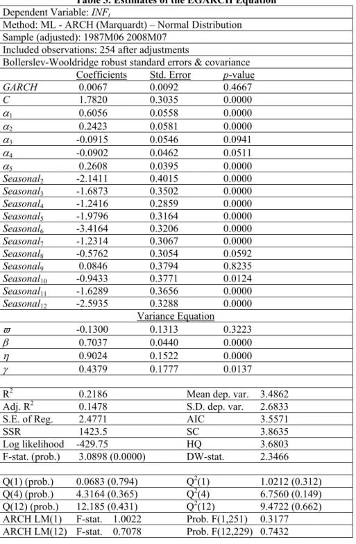
3. Conditional Volatility Estimates

Following the preliminary data issues examined in the former section, we now try to estimate the conditional mean and variance equations of the Turkish inflation. Based on the minimized Akaike information criterion (AIC), Schwarz criterion (SC) and Hannan-Quinn criterion (HQ), all information statistics propose the autoregressive order of the inflation series in the mean equation as an AR(5) process. The estimation results of the Eq. 1 and Eq. 2 estimated by the method of maximum likelihood and using Marquardt optimization algorithm as well as quasi-maximum likelihood covariances and standard errors described by Bollerslev and Wooldridge (1992) are given in Tab. 3. Consider that for the conditional distribution of the error term t, normal (Gaussian) distribution is assumed. We observe no significant effect

of conditional variance on the mean equation and also that most of the autoregressive parameters and seasonal dummies are highly significant in a statistical sense.5 _{Any estimation result that the EGARCH parameter, which}

measures the degree of how persistent is the volatility shocks, takes positive values close to one would mean that the volatility shocks are highly persistent so that conditional variance converges to the steady state quite slowly. In our case, the variance equation indicates a positive and significant EGARCH parameter as can be expected, but its coefficient, i.e. 0.70, is somewhat lower than the unit value. Since the leverage term  is positive and statistically different from zero, the news impact is asymmetric and the conditional variance of the monthly inflation reacts differently to equal magnitudes of negative versus positive shocks. Dealing with diagnostics; that all the Q-statistics are found insignificant means that the mean equation is correctly specified, and that all the squared standardized residuals are found insignificant means that the variance equation is correctly specified. Also, when the variance equation is correctly specified, there should be no ARCH effect left in the standardized residuals. ARCH LM statistics and correlogram-Q statistics estimated for the presence of autocorrelation in the standardized residuals and in the squares of standardized residuals cannot reject the null hypothesis at the conventional levels, therefore, we can infer that there exists no remaining serial correlation in the model.

5 _{Inclusion of inflation rates with two digits extreme values in the monthly basis have highly significant}

positive effects on the inflation variable in the mean equation. But, in this case, the paraemeters of the variance equation are found in an unexplanatory way. These results not reported here are available from the authors upon request.

Table 3. Estimates of the EGARCH Equation

Dependent Variable: INFt

Method: ML - ARCH (Marquardt) – Normal Distribution Sample (adjusted): 1987M06 2008M07

Included observations: 254 after adjustments

Bollerslev-Wooldridge robust standard errors & covariance

Coefficients Std. Error p-value

GARCH 0.0067 0.0092 0.4667 C 1.7820 0.3035 0.0000 1 0.6056 0.0558 0.0000 2 0.2423 0.0581 0.0000 3 -0.0915 0.0546 0.0941 4 -0.0902 0.0462 0.0511 5 0.2608 0.0395 0.0000 Seasonal2 -2.1411 0.4015 0.0000 Seasonal3 -1.6873 0.3502 0.0000 Seasonal4 -1.2416 0.2859 0.0000 Seasonal5 -1.9796 0.3164 0.0000 Seasonal6 -3.4164 0.3206 0.0000 Seasonal7 -1.2314 0.3067 0.0000 Seasonal8 -0.5762 0.3054 0.0592 Seasonal9 0.0846 0.3794 0.8235 Seasonal10 -0.9433 0.3771 0.0124 Seasonal11 -1.6289 0.3656 0.0000 Seasonal12 -2.5935 0.3288 0.0000 Variance Equation  -0.1300 0.1313 0.3223  0.7037 0.0440 0.0000  0.9024 0.1522 0.0000  0.4379 0.1777 0.0137

R2 _{0.2186 Mean dep. var. 3.4862}

Adj. R2 _{0.1478 S.D. dep. var. 2.6833}

S.E. of Reg. 2.4771 AIC 3.5571

SSR 1423.5 SC 3.8635

Log likelihood -429.75 HQ 3.6803

F-stat. (prob.) 3.0898 (0.0000) DW-stat. 2.3466

Q(1) (prob.) 0.0683 (0.794) Q2_{(1) 1.0212 (0.312)}

Q(4) (prob.) 4.3164 (0.365) Q2_{(4) 6.7560 (0.149)}

Q(12) (prob.) 12.185 (0.431) Q2_{(12) 9.4722 (0.662)}

ARCH LM(1) F-stat. 1.0022 Prob. F(1,251) 0.3177

ARCH LM(12) F-stat. 0.7078 Prob. F(12,229) 0.7432

Below we give the graph of the conditional variance series extracted from the EGARCH equation:

0 1 0 2 0 3 0 4 0 5 0 6 0 8 8 9 0 9 2 9 4 9 6 9 8 0 0 0 2 0 4 0 6 0 8 C o n d i t i o n a l v a r i a n c e

Figure 2. Graph of the Conditional Variance

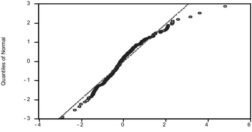
Plotting the quantiles is another way to examine the distribution of the standardized residuals. If the residuals are normally distributed, the points in the Quantile-Quantile plots should lie alongside a straight line. By setting identical axes to facilitate comparison with the diagonal line, we see in Fig. 3 below that especially large positive, and to some extent negative shocks, drive the departure from normality. - 3 - 2 - 1 0 1 2 3 - 4 - 2 0 2 4 6 Q u a n t i l e s o f S t a n d a r d i z e d R e s i d u a l s Q u ant ile s o f N orm al

Figure 3. Quantile-Quantile Graph

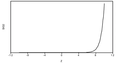
Having estimated the model, we now plot the News Impact Curve (NIC). Our goal here is to plot the volatility against the impact z =  /  where:

log(t2) =  +  log(t-12) + z t-1+  zt-1 (3)

We fix last period’s volatility t-12 to the median of the estimated conditional

- 1 2 - 8 - 4 0 4 8 1 2 Z

SI

G

2

Figure 4. News Impact Curve (NIC) of the Inflation Conditional Variance

Above SIG2 is used for the 2 _{series and z indicates an equispaced series between 10}

and -10. In Fig. 4, an asymmetric leverage effect can easily be observed. More explicitly, such a finding means that the conditional variance of the inflation reacts more to past positive shocks than to negative innovations of the equal size. The economic consequence of this finding is that inside the period under investigation, an unanticipated increase in inflation would lead to a higher level of uncertainty when compared with the level of uncertainty resulted from an unanticipated decrease in inflation.

4. Granger Causality Analysis

Next, for the temporal ordering between the Turkish inflation and inflation uncertainty, for which the latter is represented by the conditional variance series produced above, we implement the Granger-causality tests. In this manner, we aim to reveal the knowledge of whether the Friedman-Ball hypothesis that requires a causal / precedence relationship running from inflation to its uncertainty, or the Cukierman and Meltzer hypothesis that states a reverse causal relationship running from uncertainty to inflation, or both can be supported by the actual data. The Granger causality between the two variables, say X and Y, asks that how much of the current X can be explained by a regression on its past values, and then tries to test whether inclusion of the lagged values of Y into the regression to explain X have statistical significance as a whole. If so, we can infer that Y helps predict the course of X, or in other words, X is Granger-caused by Y. More formally, to test the causal relationship between inflation (INFt) and inflation uncertainty (INFUNCt), let us

write down the bivariate regressions as follows:









where co denotes the constant term in the Granger regressions, n represents the lag

length chosen for causality analysis, which is assumed in principle to correspond to the expectations for the longest time over which variables could predict the others, and t and ut are assumed as white-noise error terms in the regressions. Note that the

null hypothesis in Eq. 4 is that the lags of INFUNCt are not significant as a whole,

that is to say, INFUNCt does not Granger-cause INFt. Likewise, the null hypothesis

in Eq. 5 is that the lags of INFt have no statistical significance in explaining

INFUNCt, which also means that INFt does not Granger-cause INFUNCt. By

employing F-type Wald tests, the results of pairwise Granger causality analysis which are applied on the joint significance of the sum of lags of each explanatory variable are reported below.6 _{For this purpose, various lag lengths are considered to}

see whether the estimation results are sensitive to the a priori lag selection.

Table 4. Granger Causality Tests for Inflation and Inflation Uncertainty

Lag H0: INFt does not Granger-

cause INFUNCt

H0: INFUNCt does not Granger-

cause INFt 3 45.2476*** _{(+) 2.0933 ()} 6 24.3639*** _{(+) 0.9660 ()} 12 14.6688*** _{(+) 2.0940}** _() 18 12.6164*** _{(+) 1.6332}* _() 24 11.6198*** _{(+) 3.1716}*** _()

The statistics in Tab. 4 belong to the F-type Wald tests. The asterisks ***_, **_{, and} *

indicate significance at the 0.01, 0.05 and 0.10 levels, respectively. The signs (+) and () are used for the process by which the sum of the coefficients of Granger equation yields a positive or negative sign, respectively. In Tab. 4, we can easily notice that the null hypothesis that inflation does not Granger-cause inflation uncertainty is rejected at the 0.01 significance level, no matter how long the lag length is. In other words, we find that inflation does precede the course of the inflation uncertainty. When the sign of the sum of the coefficients given in parentheses are examined, the total effect of inflation on inflation uncertainty turns out to be positive, a result that supports what the Friedman-Ball hypothesis adduces. However, no clear-cut evidence in the opposite direction can be found. The hypothesis that inflation uncertainty Granger-causes inflation cannot be rejected for only three of the five lag lengths considered in the causality analysis. But, we can infer that the larger the time period, the more significant in a statistical sense is the causal relationship running from the inflation uncertainty to the level of inflation. The sum of the coefficients in all lag lengths in this case turns out to be negative, which means that increased uncertainty in inflation tends to precede a decline in the level of inflation. Holland (1995) explains as a possible reason of this case that an increase in inflation uncertainty can be viewed by policymakers as costly, so induces them to fight inflation to reduce it in the future. Nas and Perry (2000) also touchs upon the issue that inflation and associated uncertainty create real costs, which lead policy authorities to monetary tightening stabilization efforts to lower inflation.

6 _{Following Nas and Perry (2000) and Daal et al. (2005), since Granger causality tests initially indicate}

the temporal ordering or precedence relationship between each variable but do not reveal the sign of this relationship, we also give below the sign of the sum of the coefficients taken from each Granger equation to determine whether the Granger causality, if estimated, is in the positive or negative way.

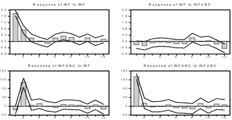
To further control the direction of the relationship between inflation and its uncertainty, we apply to the generalized impulse response (GIR) analysis proposed by Koop et al. (1996) for non-linear dynamic systems and further developed by Pesaran and Shin (1998) for linear multivariate models. Briefly to say, we can consider the impulse response functions as the path whereby the variables return to their equilibrium values (Green, 2000), if so, also supporting their stationary characteristics. The GIR analysis can be considered an alternative to orthogonalized impulse responses. The GIRs which take account of the historical patterns of correlations observed among different shocks provide researchers to be invariant to the ordering of the variables in the system. For this purpose, we construct initially an unrestricted VAR(12) system.7 _{The generalized impolse response estimates of the}

inflation and inflation uncertainty using 2000 Monte Carlo repetitions of 2 standard deviations (s.d.) are reported below.

- 0 . 8 - 0 . 4 0 . 0 0 . 4 0 . 8 1 . 2 1 . 6 2 . 0 2 4 6 8 1 0 1 2 R e s p o n s e o f IN F t o IN F - 0 . 8 - 0 . 4 0 . 0 0 . 4 0 . 8 1 . 2 1 . 6 2 . 0 2 4 6 8 1 0 1 2 R e s p o n s e o f IN F t o IN F U N C - 4 0 0 4 0 8 0 1 2 0 1 6 0 2 4 6 8 1 0 1 2 R e s p o n s e o f IN F U N C t o IN F - 4 0 0 4 0 8 0 1 2 0 1 6 0 2 4 6 8 1 0 1 2 R e s p o n s e o f IN F U N C t o IN F U N C R e s p o n s e t o G e n e r a li z e d O n e S . D . I n n o v a t i o n s ± 2 S . E .

Figure 5. Generalized Impulse Response Functions

In. Fig. 5, we find that both inflation and inflation uncertainty respond in a statistically significant way to their own shocks. This is not surprising in a chronic-high inflationary country which can be expected, to the great extent, to have been subject to the price inertia phenomenon. When we consider the dynamic interactions between inflation and its uncertainty, we observe that a one s.d. positive shock to the inflation leads to a highly significant increase in inflation uncertainty in the second period following the shock. Given the symmetric nature of impulse responses, we can infer that a decrease in inflation would also lead to a decrease in the associated uncertainty. On the other side, however, we are unable to find an explicit significant impact of inflation uncertainty on inflation except the 12th _{period following the}

shock. Note that the significance of the impact of initial shocks occured on inflation

7 _{Using the maximum lag length 12 for the monthly frequency data, both the minimized Akaike}

information criterion (AIC) and sequential modified LR test statistics employing small sample modification suggest to use the lag order 12 for the unrestricted VAR model. Furthermore, the largest root of the characteristic polynomial for the VAR model is 0.9938, therefore it satisfies the VAR stablity condition that enables us to implement impulse response analysis for the dynamic interactions between the variables. Note that statistical significance of the impulse response functions coincides also with the case that the upper and lower confidence bands carry the same sign.

uncertainty upon the inflation lies in a negative way throughout the upper confidence bands. These all give support to the Friedman-Ball hypothesis considered in the former sections.

5. Concluding Remarks

The Turkish economy has witnessed a chronic two-digit inflation for the post-1980 period and this constitutes an important benchmark for economic agents in constructing their expectations as for the future periods. In this paper, we have attempted to investigate one of the main properties of inflation, that is, whether there exists any preceding / causal relationship between inflation and inflation uncertainty. Our estimation results indicate that inflation in fact leads to inflation uncertainty in line with the Friedman-Ball hypothesis. Dealing with the information content of this relationship, we find that the conditional variance of the Turkish inflation reacts more to past positive shocks than to negative innovations of equal size. The causality analysis reveals that inflation Granger causes, or in other words precedes, inflation uncertainty, but no clear-cut evidence in the opposite direction in a statistically significant way can be found. Finally, these findings have also been supported by the generalized impulse response analysis. Complementary future papers should be constructed to examine the effects of transition to an explicit-inflation targeting framework on the explicit-inflation-explicit-inflation uncertainty relationship.

References

AKYAZI, H., ARTAN, S. (2004). Türkiye’de enflasyon-enflasyon belirsizliği ilişkisi ve enflasyon hedeflemesinin enflasyon belirsizliğini azaltmadaki rolü. Türkiye Bankalar

Birliği Bankacılar Dergisi, Mart, sayı 48, 3-17.ss.

BALL, L., CECCHETTI, S.G. (1990). Inflation and uncertainty at short and long horizons.

Brookings Papers on Economic Activity, vol. 1, pp. 215-254.

BALL, L. (1992). Why does higher inflation raise inflation uncertainty?. Journal of

Monetary Economics, vol. 29, pp. 371-378.

BOLLERSLEV, T. (1986). Generalized autoregressive conditional heteroskedasticity.

Journal of Econometrics, vol. 31, pp. 307-327.

BOLLERSLEV, T., WOOLDRIDGE, J.M. (1992). Quasi-maximum likelihood estimation and inference in dynamic models with time varying covariances. Econometric Reviews, vol. 11, 143-172.

CAPORALE, T., MCKIERNAN, B. (1997). High and variable inflation: further evidence on the Friedman hypothesis. Economics Letters, vol. 54, pp. 65-68.

CUKIERMAN, A. (1992). Central bank strategy, credibility, and independence. MIT Press, Cambridge.

CUKIERMAN, A., MELTZER, A. (1986). A theory of ambiguity, credibility, and inflation under discretion and asymmetric information. Econometrica, vol. 54, September, pp. 1099-1128.

DAAL, E., NAKA, A., SANCHEZ, B. (2005). Re-examining inflation and inflation uncertainty in developed and emerging countries. Economics Letters, vol. 89, pp. 180-186.

DAVIS, G.K., KANAGO, B.E. (2000). The level and uncertainty of inflation: results from OECD forecasts. Economic Inquiry, vol. 38, no. 1, pp. 58-72.

DEVEREUX, M. (1989). A positive theory of inflation and inflation variance. Economic

Inquiry, vol. 27, January, pp. 105-116.

ENDERS, W. (2004). Applied econometric time series. Wiley&Suns, Inc.

ENGLE, R.F. (1982). Autoregressive conditional heteroskedasticity with estimates of the variance of U.K. inflation. Econometrica, vol. 50, pp. 987-1008.

ENGLE, R.F., LILIEN, D.M., ROBINS, R.P. (1987). Estimating time varying risk premia in the term structure: the ARCH-M model. Econometrica, 55, 391–407.

ERTUĞRUL, A., SELÇUK, F. (2002). A brief account of the Turkish economy. In: A. Kibritçioğlu, L. Rittenberg and F. Selçuk (eds.), Inflation and disinflation in Turkey, Ashgate Publishing Limited, pp. 13-40.

FOUNTAS, S. (2001). The relationship between inflation and inflation uncertainty in the UK: 1885-1998. Economics Letters, vol. 74, pp. 77-83.

FRIEDMAN, M. (1977). Nobel lecture: inflation and unemployment. Journal of Political

Economy, vol. 85, no. 3, pp. 451-472.

GREEN, W.H. (2000). Econometric analysis. Prentice-Hall, Inc.

GRIER, K.B., PERRY, M.J. (1998). On inflation and inflation uncertainty in the G7 countries. Journal of International Money and Finance, vol. 17, no. 4, pp. 671-689. GRIER, K.B., PERRY, M.J. (2000). The effects of real and nominal uncertainty on

inflation and output growth: some Garch-M evidence. Journal of Applied

Econometrics, vol. 15, no. 1, pp. 45-58.

HENRY, Ó. T., OLEKALNS, N., SUARDI, S. (2007). Testing for rate dependence and asymmetry in inflation uncertainty: evidence from the G7 economies. Economics Letters, vol. 94, pp. 383-388.

HOLLAND, A.S. (1995). Inflation and uncertainty: tests for temporal ordering. Journal of

Money, Credit, and Banking, vol. 27, no. 3, pp. 827-837.

HWANG, Y. (2001). Relationship between inflation rate and inflation uncertainty.

Economics Letters, vol. 73, pp. 179-186.

KİBRİTÇİOĞLU, A. (2002). Causes of Inflation in Turkey: A Literature Survey with Special Reference to Theories of Inflation. In: A. Kibritçioğlu, L. Rittenberg and F. Selçuk (eds.), Inflation and disinflation in Turkey, Ashgate Publishing Limited, pp. 43-76.

KONTONIKAS, A. (2004). Inflation and inflation uncertainty in the United Kingdom, evidence from GARCH modelling. Economic Modelling, vol. 21, pp. 525-543.

KOOP, G., PESARAN, M.H., POTTER, S.M. (1996). Impulse response analysis in nonlinear multivariate models. Journal of Econometrics, vol. 74, pp. 119-147.

NAS, T.F., PERRY, M.J. (2000). Inflation, inflation uncertainty, and monetary policy in Turkey: 1960-1998. Contemporary Economic Policy, vol. 18, no. 2, pp. 170-180. NELSON, D.B. (1991). Conditional heteroskedasticity in asset returns: a new approach.

Econometrica, vol. 59, no. 2, pp. 347-370.

NEYAPTI, B., KAYA, N. (2001). Inflation and inflation uncertainty in Turkey: evidence from the past two decades. Yapı Kredi Economic Review, vol. 12, no. 2, pp. 21-25. OKUN, A. (1971). The mirage of steady inflation. Brookings Papers on Economic

Activity, vol. 2, pp. 485-498.

ÖZDEMİR, Z.A., FİSUNOĞLU, M. (2008). On the inflation-uncertainty hypothesis in Jordan, Philippines and Turkey: a long memory approach. International Review of

Economics & Finance, vol. 17, no. 1, 2008, pp. 1-12.

ÖZER, M., TÜRKYILMAZ, S. (2005). Türkiye’de enflasyon ile enflasyon belirsizliği arasındaki ilişkinin zaman serisi analizi. İktisat İşletme ve Finans, 5, (229) 93-104.ss. PESARAN, M.H., SHIN, Y. (1998). Generalized impulse response analysis in linear

multivariate models. Economic Letters, vol. 58, pp. 17-29.

TELATAR, F. (2003). Türkiye’de enflasyon, enflasyon belirsizliği ve siyasi belirsizlik arasındaki nedensellik ilişkileri. İktisat İşletme ve Finans, cilt 18, sayı 203, 42-51.ss. TELATAR, F., TELATAR, E. (2003). The relationship between inflation and different

sources of inflation uncertainty in Turkey. Applied Economics Letters, vol. 10, no. 7, pp. 431-435.