Network model approach to the analysis of multirigid-body systems

Dynamics and Control 3, 107-125 (1993) 9 1993 Kluwer Academic Publishers, Boston. Manufactured in The Netherlands.

Network Model Approach to the Analysis of

Multirigid-Body Systems

YILMAZ TOKAD*

Department of Mathematics, Bilkent University, 06533 Bilkent, Ankara, Turkey Received April 17, 1991; revised December 3, 1991 and February 4, 1992 Editor: W, Stadler

Abstract. The mathematical model of a rigid body in three dimensional motion developed in [1] is used to for- mulate the equations of motion for the systems o f rigid bodies connected to form a special type of open kinematic chain. In this interconnection pattern of rigid bodies, each rigid body is considered as a 3-port component, and for the sake of generality, initially no constraints are imposed on the joints used to interconnect the rigid bodies. The system is considered as an (m + 1)-port component and the corresponding terminal equations are obtained in closed form. As an appliction of these equations, a three-link plane manipulator is considered.

1. Introduction

In an earlier article [1], a mathematical model of a rigid body in three-dimensional motion as a multi-terminal component is derived. In this derivation, an approach widely considered and applied in the analysis of electrical networks is used. In this article the same approach is applied to the formulation of the equations of motion for a system of interconnected rigid bodies. To be more specific, here the application is restricted to a system of special type of interconnected rigid bodies possessing an open kinematic chain. Such a system actually appears in various kinds of manipulators. The system itself is considered as an (m + 1)- port mechanical component and modeled in such a way that the corresponding terminal equations are obtained in closed form.

The simplest form of the terminal equations of a rigid body corresponding to a star-like tree (a terminal graph) with k branches is given by equation (42) of [1]. In what follows, these equations are reproduced for k = 2. With this restriction we actually assume that each rigid body (6lj) in the system is to be connected to, at most, two adjacent rigid bodies ((Rj_0 and ((Rj+I) at its designated ports (O

Aj) and (0 Bj).

Therefore, each rigid body ((Rj) (see Figure la) will be considered as a

three-port

component which is represented by the schematic diagram shown in Figure lb, and its terminal equations corresponding to the terminal graph in Figure lc will be in the following form:

%

Y~ 012,12

I

-Kbj

I

Wafld/dt)J

L xtj J

012,1 u~ (1)

where all the submatrices

E'I

i iot

E IOl

i mJ, l

Kaj = RGaj I , Kbj = RGb j I , UGj = 0

"

[ ~ 1 7 6

Waj = e G j ~ + QG 1,Pay = , Q~j =

JGj

o %/G s

(2)

contain 6 rows, x . , y . , UG. are column matrices, while the 6 x 6 matrices are patitione _{PJ Pi y} into 3 • 3 submatrices. If the rigid body is assumed to be ideal, in equation (1) the 6 x 6 operator matrix WG,(d/dt) and the column matrix u~ are replaced by appropriate zero matrices yielding the terminal equations of the ideal rigid body ((R0j) as

O12,12 ]

h

- -

t

Y~ ] -Kaj --Kb~ [ 06,6

(3)

This observation permits us to represent the three-port rigid body as the interconnection of an ideal rigid body ((R0j), and an active one-port mechanical component with the ter- minal equations of the form

= WGj ' (4)

Y6 i xa s + UG i

and as indicated in the schematic diagram in Figure ld, where the active one-port compo- nent is further decomposed into the parallel interconnection of two one-ports, (Woj) and (ua), the latter being a through driver (source) corresponding to the force and torque due to dae gravity. Stated differently, the kinetic property of rigid body ((Rj) can be represented by the addition of an active one-port component, having the terminal equations in (4), to the (OGj) port of an ideal rigid body ((Roy). One may also be interested in knowing whether the active component can be moved to any one of the other ports (OBj) or (OAj) of the ideal rigid body ((Roj), so that the new interconnection configuration still represents the same rigid body ((Ry). This is indeed possible, however, with the distinction that the coef- ficientmatrices WG: and u@ in equation (4) are now replaced by different ones as indicated in the schematic diagrams of Figures le and lf. This property follows from the fact that in equation (1) both of the submatrices Ka. and Kb. are nonsingular and the terminal equa-

l/ 3 . . .

NETWORK MODEL APPROACH TO THE ANALYSIS OF MULTIRIGID-BODY SYSTEMS 109

%

- 4

012,12 (K~I) r --gbbj 1 WBj

x~

O12,1 +

UBj

(5) and

x~

012,p.

+

1

O12,1 _ K ~ I K~ -1 ~j UAj (6) where

i I 01 [, 01 [, 01

KAj = KaJ Kaj = Rrbj I R6a j I Rj I " (7)

The expressions of the other submatrices in equations (5) and (6) are given by equations (49) and (50), in the appendix, respectively.

The forms of the terminal equations of a three-port rigid body given in equations (1), (5), and (6) are all equivalent. In a systematic formulation of the equations of a system of rigid bodies, it may be necessary to select a particular and perhaps dafferent form of the terminal equations for each rigid body in the system. As indicated in [1], the ideal rigid body (fft0j) with terminal equations given in (3) corresponds to a three-port ideal transformer in network theory. Therefore, a topological necessary condition which is well established in network theory [2-7] for the unique solvability of the networks containing ideal transformers can also be applied for the systems of rigid bodies. Considering the three possible forms of the terminal equations of a rigid body in equations (1), (5), and (6), we then state that in the system graph drawn for a system of rigid bodies there must exist a formulation tree T such that only two of the edges of the terminal graph for each rigid body (shown in Figure lc) should be contained in T while the third edge be contained in the co-tree T' of T.

There is another topological necessary condition on the classifications of the edges cor- responding to the drivers is [2, 8]: For the existence of a unique solution of the system equations, all the edges in the system graph corresponding to the across drivers must be included in every formulation tree Twhile all the edges corresponding to the through drivers must be in the co-tree T' of T.

Bj,

A)

Bj ~ G j

9

o

o

( o ) ( b ) (c)

(UGj)

9 ~ (WGj) ,

"-"

B j ~

oAj

0

G~

(

%i

)

B ~

_,___L .~_ o

Gj

B~ A~

( UAj ) ( d ) Ce) ( f )

Figure 1.

(a) Three-port rigid body (d{j) with the joint terminals

Aj, Bj

and the terminal

Gj

corresponding to the center of mass of

((~-j).

(b) Pictorial representation of (~j).

(c) The terminal graph of the three-port (~j).

(d) Three-port rigid body (61j) is represented as an interconnection of ideal rigid body

((Roj)

with the terminal equations in (3) and an active one-port component with the terminal equations in (4), (e) Active one-port component at port (Gj0) is moved to the port

(BjO).

(f) Active one-port component at port

(GjO)

is moved to the port

(AjO).

2. The systems of rigid bodies

In this section the system of rigid bodies ((Rj) ( j = 1, 2 . . . m) (see Figure 2a) will be of interest where each rigid body is regarded as a three-port component with ports

(Aj,

0), (Bj, O) and (Gj, 0).

Such systems are useful in robotic studies [9]. In this system, the terminal

Aj

o f ((Rj) is assumed to b e connected to the terminal

Bj+I

o f ((Rj+I) ( j = 0, 1 . . . . , m - 1) to form an open kinematic chain. In the following, this system will be modeled as an (m + 1)-port component, one of the ports being

(Am,

O) and the remain- ing ports corresponding to the interconnected terminal pairs

(Aj, Bj+ 0

of the rigid bodies ((Rj) and ((Rj+I), respectively; i.e., in the model, the terminal graph will of the form shown in Figure 2b. Note, the terminal graph is disconnected (separated). At the beginning, we shall save the mass centers of the rigid bodies as additional terminals; therefore, we first consider the enlarged terminal graph given in Figure 2c. In order to obtain the terminal equations in the desired closed form corresponding to the terminal graph in Figure 2c,

NETWORK MODEL APPROACH TO THE ANALYSIS OF MULTIRIGID-BODY SYSTEMS 111

this system must be excited by (2m + 1) drivers (1"), (2*) . . . . , (m*), (m + 1)* (1") ', (2*) ', 9 (m*)' at the ports which are dictated by the edges of this terminal graph. The schematic diagram of the system augmented with the (2m + 1) drivers is given in Figure 2d and the corresponding system graph will be as in Figure 2e. Note, in an actual system no connec- tions are made to the ports (Gj, O) and, hence, even if we assume that the drivers (j*)'

are connected to these ports, the through variables (y*)' (i.e., forces ( f T ) ' and torques (M 7 ) ' ) of the drivers are identically equal to zero. However, as can be seen from the system graph (see Figure 2e), the across variables of the drivers are equal to the aross variables xGi at the ports (Gj, O). Although these across variables are to be eliminated in the final expression of the terminal equations, their use as auxiliary variables will result in some simplifications in the expressions we will be dealing with. From the system graph (see Figure 2e), the following observations can be made:

( ~ ) - E ' ~ A

I

'

o!'t k

o ... b? ?" o ~ 3 ~o

(a)

(b)

(c j-~ f i . ' f

%d>_ ~

i m;1

g*~g=

(C)

_%~

(3")

(d)

(e)

Figure 2. (a) The system of m rigid bodies.

Co) The terminal graph associated with the terminal equations in (20). (c) The terminal graph associated with the terminal equations in (21).

(d) A pictorial diagram of the system of rigid bodies in Figure l(a) augmented with the through (force- moment) drivers (1"), (2"), ..., (mr*) and the across (velocity) drivers (1") ', (2*) ', .... (m*) ', and (m + 1)*.

In the system, for each rigid body, let the form of the terminal equations: (i) in equation (1) be used.

(ii) in equation (5) be used. (iii) in equation (6) be used.

Then the topological conditions for the existence of a solution, as discussed at the end of the Introduction, implies for each case that

(i) the edges (a i, o), (bi, o) q = 1, 2, . . . , m) are included in a formulation tree T while the edges (gi, o) (i = 1, 2 . . . m) are in the co-tree T'. Therefore the edges (1"), (2"), . . . , (m*) are necessarily in T ' while the edges (1") ', (2*) ', . . . , (m*) ', and (m + 1)* are included in T. These two groups of edges must correspond to through and across drivers, respectively.

(ii) The edges (a i, o), (gi, o) (i = 1, 2, . . . , m ) are included in T while the edges (bi,

o) (i = 1, 2, . . . , m) are in T'. In this case the edges (1"), (2"), . . . , (m*) must corre- spond to across and the edges (1") ', (2*) ', . . . . (m*)' and (m + 1)* must correspond to through drivers.

(iii) In this case the edges (bi, o), (gi, o) (i = 1, 2 . . . . , m) will be in T and the edges

(ai, o) (i = 1, 2, . . . , m) will be in T '. Hence the edges (2"), (3*) . . . (m + 1)* correspond to across while the edges (1"), (1")', (2*) ', . . . , (m*)' correspond to through drivers.

The desired terminal equations can be obtained by considering any one of the three cases considered above. In application, however, at the joints the displacement variables and at the port (Am, O) the mechanical load (the force fm+l and torque Mm+ 1) variables are specified. Therefore, the proper choice of drivers is that of case (ii). However, the operator matrix WB in equation (5) has rather complex expression compared to Wa in equation

J . . . ~ .

(1). For this reason, the following formulation wall consider the type of excitation discussed in case (i); i.e., in the system graph, the formulation tree will necessarily be as shown by the thick lines in Figure 2e.

Note, to keep the analysis valid under fairly general interconnection conditions, the types of joints (element pairs) to be used for connecting the rigid bodies in the system are not specified in advance. The special cases where the joints are spherical, revolute and prismatic (sliding pair) are considered after the establishment of the general system model. Although the closed form equations are useful for theoretical investigations, an algorithmic approach to the solution of these equations is preferable [10-14]. This is the main reason for keep- ing the across variables xc. associated with the ports (Gj, 0 ) .

From the system graph ~see Figure 2e), the fundamental circuit equations are

X * I =

Xbl

t

Xj* = Xbj - - X a ( j _ l ) ( j = 2, 3, . . . , m) x(j.), = X Gj ( j = 1, 2 . . . m) X ( m + l ) * ~

Xa m

J

(8)

NETWORK MODEL APPROACH TO THE ANALYSIS OF MULTIRIGID-BODY SYSTEMS 113

and the fundamental cut-set equations are,

Yj* +Ybj = 0 ( j = 1 , 2 , . . . , m ) - ]

Yaj

= yb(;+u. ( j = 1, 2, . . . , m -- I)

)

YGj + Y~j*)' = 0 ( j = 1 , 2 . . . m) . Ya m + Y(m+l)* = 0 YC/*)' -- 0 ( j = 1, 2 . . . m) (9)

F r o m the first six rows of equation (1) we get r.-T . K - 1 . Z

Xaj = l~ajl, by ) Xbj = (Kbj 1 Kaj)Txbj =

Kra~Xbj

(10) and the circuit equation (8) and the relations in equation (10) thus yield

Xl* X2* Xm* X(m+l)* I -K~ t T --K~l(m_l ) I

x 2[

Xbm A = [KllXB'K2

(11)

Note that the 6m • 6m submatrix K 1 is nonsingular, while K2 is a 6 • 6m submatrix. By considering the second row block in equation (1), we write

x s = Xb Xb 2 xbm

G

x~ 1

x ~ XGm = KdXo (12) where the coefficient matrix Kd is nonsingular. Substituting equation (12) into equation (11) we obtain

6m Ex* 1 I ll

_{(6) x(m+ 0* = K2 KdxG = K ' x 6 (13)}

where the submatrix K = KIKd is nonsingular. On the other hand, f r o m the last six rows of equation (1) we have

If this set of equations is put into one matrix equation form and considering the fundamen- tal cut-set equations in equation (9) we obtain

XG 1

XG,,

I Yl*

Kb~ L Y,~* UG 1

uG,,

b I - K a 1

Kb~

- K a ( m _ l )

I

I

I

YI*

Ym*

Y(m+

1)*

UG 1 UG 2

u6,.

(15)

or in a more compact form

[y*]

= - - ua. (16)

W6x~

[KT (K')r]

Y~m+l)*

Since the terminal variables and the variables corresponding to the drivers are related by

Ix]__

x(m+

1)

Xl X2 Xra x(m+

1)

Xl*

X2*

Xm*

X(m+l)*

,EyyI

_(m+l)

Yl

Y2

Ym

Y(m+

1)

Yl*

Y2*

Ytrt*

Y(m+ 1)

(17) from equations (13) and (16) we obtain the intermediate form of the terminal equations as

(6) XCm+l) K '

(6)

W6x~= [KT (K')T] I

Y 1

Y(m+l)

- - U G

(18)

Note, as stated above, the 6m • 6m submatrix K = K1K d is nonsingular and the explicit

form of its transpose appears in (15). Therefore, if we let S = K -l, then the expressions of the 6 • 6 submatrices Spq ( p ,

q = 1, 2, ..., m)

of S are given as follows,

NETWORK M O D E L APPROACH TO THE ANALYSIS OF MULTIRIGID-BODY SYSTEMS 115

Spq = O p < q ) S p q = I p = q Spq _{= (Kffp)(K:4(p_I~)(KA(,_2))...(} - 1 T T T KTA~ _{p > q}

(19)

In equation (18) the auxiliary variables x G can be eliminated. Indeed, from the first rela- tion in equation (18) we have xo = K - i x = Sx and Xm+l = K 'Sx, hence the second rela- tion becomes Wc, Sx = Kry + (K 3ry(m+l ) - u G. These relations may be written together in the following single matrix form

,6m,

₍₆₎

I y I I

_{X(m + 1) K 'S 0}

I x ]+IS luo

_{Y(m+ 1)}

These are the terminal equations corresponding to the terminal graph in Figure 2b of the rigid body system considered as (m + 1)-port component. However, the terminal equa- tions of the rigid body system, augmented by the ports (OGj) ( j = 1, 2 . . . m) corre- sponding to the terminal graph in Figure 2c, can also be given. Indeed, assuming that the yGjs are not zero, and since xo = Sx, we have

,6m, lyl

(6) XCm+a ) = 0 0

lxl li t

Y(m+l) +

(6m) x6 0 0 Ya

uo. (21)

Taking Yo =- 0, this equation reduces to equation (20).

2.1. Forward dynamics

The equations (18) are called forward dynamics equations of the rigid body system. In- deed, if all the through variables (y, Ym+l and u6) are specified, then the motion of the system is determined; i.e., from these equations, once the across variables (velocities) x6 associated with the mass centers are determined, the joint velocities are obtained. In fact, if we let W = SrWG S = Sr(Pc~tt + O6)S = p d + Q dt where

P = sre~

d )

Q = ST"(Qc, S + Pc--~tt S)

then the first 6m rows of equation (20) can be put into the form

(22)

(23)

e d x + (Qx - (K'S)ry,n+l-y) + SrUG = 0

which represents the equations of motion of the system in closed form. However, to obtain the final form of these equations, position and velocity dependent coefficient matrices together with the joint velocities x in equation (24) must be expressed in terms of generalized coordinates which may be chosen for this system and represented by a column matrix q of order 6m, i.e., 3m components of q correspond to the joint displacements ~, and the other 3m components correspond to the joint angular displacements/9. More specifically, from equation (2) and the expression for W in equation (22), it follows that the entries in P, (K 'S) T and S are functions of q while the entries in Q are functions of both q and

x = d/dt q; i.e., the relations in equation (24) yields 6m second order differential equa-

tions in 6m generalized coordinates. Note the square coefficient matrix P in equation (24), the inertia matrix of the system, is symmetric and positive definite. This property is evi- dent from equation (23) and the expressions of PGj and W G in equations (2) and (16), respectively where PGj is symmetric and positive definite.

2.2. Explicit forms of the coefficient matrices in equation (24)

The explicit forms of P and Q in equation (24) are rather cumbersome as will be seen from the following expressions. Considering equations (19) and (23) we have

p =

sT2 "'" sT2

PG2

$21 S22 . (25)

r Smt S, n2 . S,,~

S~n PG~ ""

Therefore a typical 6 • 6 block entry Ppq of P is

Ppq = ~7=~SfpPGjSjq"

~ ol = max(p, q).

(26)

Note that since j -> p or q, equations (7) and (19) together result in

E

I ~ k ~ q R ~ + R c , oj

j

= "K-IxTKT K~

. KTq

--- (27)

Sjq

\ bj

J A(J -1) A(J - 2 ) ' " 0 I "

Substituting the expressions of PGj appearing in equation (2) together with equation (27) into equation (26) yields the following explicit expression for Ppq:

I

mfl

rnj(~k=qRk)+RGb

T~

1

= m "--1R DT ~:~.~-1 DT " Ppq ~=,~ mj(,YJk=p - 1

Rk

+ Rrc, b) JGj + mj(Z/k=p k + l~'Gbjlk k=q'"k + RGbj)

(28)

'-1

R

RTbj and rj-1

R T

The submatrices ~=p k + ~=q k -[- RGbj in equation (28) can be modified

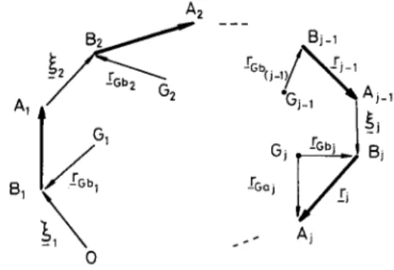
somewhat. Indeed, considering Figure 3, we define

= "-1 R

NETWORK MODEL APPROACH TO THE ANALYSIS OF MULTIRIGID-BODY SYSTEMS 117 A~ B1 A2

B2

rGb~i_~/~_~i_ ~

"Gi_; ~, Ai_~

Gj "-FGb} gj 1 -rG,:i o

Figure 3.

Vectors

rj, rGj and ~j

associated with the system in Figure la.

where the 3 x 3 skew symmetric matrix ~k represents the position vector (k of B k relative to Ak-1 while Rp ~] corresponds to the position vector of Gj relative toBp. T h e term Rq G. iS similarly defined9 In the case of spherical joints [15] ~k - 0 and using equation (29) with Ek - 0 in equation (28), we have

E

mjI

m"

r,

jgq,Gj

1

m r ; a = m a x ( p , q).

epq = Z?=et mjRe,Gj J~j + ,,.jRp,GRq,6j

(30)

Note that in equations (28) and (30) m denotes the number of rigid bodies in the system, while mj is the body mass. Carrying out similar operations, explicit expression for the coefficient matrix Q in equation (23) can be given. However, in order to keep its com- plicated appearance relatively low, derivatives of matrices in equation (23) are not replac- ed by the relations d/dt R = fiR - Rf~ given in A. 12 of the appendix of [1]. Note, the second term Rfl on the right may be omitted due to its multiplication by o~ in the final expressions; i.e.,

E ~

~(..0 "~- (.0 3 0 --W 1 O~ 2 ~ 0 9 - - ~ 2 0)1 0 W 3

0

mj --~(~k=qRk + RGbj)

"-t r d "-1 T ;

apq = ~'~n=a

0 ~G/Gj -[- mj(~k=pg k + eGbj)--~(~k=qek + gGbj)

o~ = max(p, q) (31) In the case of spherical joints, we have

apq : ~,?=ct

d T

0

mj --~tteq,Gj

d r

0

~G/Gj + mjep,Gj-~ttgq,G j

; ot = max(p, q). (32)

On the other hand, when the rows of the last column matrix u =

Sruc

in equation (24) are partitioned into m column matrices of order 6, the p-th one is

m r

I rnj(F-~-~p mjI+

1

(33)

= r,~=pSj~uaj = -E'fl=,

Rk R~j)

g

Up

or in the case of spherical joints,

= - - F , m [ m j l ?

u@

.j =p mjRp,G

j

g.

(34) To complete the explicit expressions of various submatrices appearing in equation (20), consider the last block of rows:

X(m+l ) - - - - (K'S) = Kam[Sml Sm2 . . . Smm ] x . r (35)

Utilizing the expression in equation (27) with j and q replaced by m and j, respectively, equation (35) takes on the form

E

El

X(m+l) =

KTm

~7=lSmjX j =

~mT=l OI ki:'k

wjVj

(36)

Note, in the case of spherical joints, since the joint velocities

vj

are zero, the first column blocks of the coefficient matrices appearing in equations (28), (30), (31), (32), and (36) may be omitted. In the case of sliding joints, the second column blocks of the same coeffi- cient matrices may be omitted. In the case of spherical joints, the position vector of

A m

relative to

Bj

is

Rj, m = ~tff=jR k

and the relation in equation (36) becomes

X(m+I) = [ Vm+l ? = I R ~ I m " ' " O)m+ 1 " 9 9 (37) Rmm

I

1

(.0 m

(38)

Furthermore, if we let 60j = njwj where

nj

indicates the unit vector in the direction of wj, then equation (38) may be put into a more compact form

X ( m + l ) =

mnmJ El

39

V RTrnnl r 601 1_ nl 9 . . n m

r m

NETWORK M O D E L APPROACH TO THE ANALYSIS OF MULTIRIGID-BODY SYSTEMS 119

2.3. Inverse dynamics

The terminal equations (20) can be interpreted in various directions. First, if the linear and angular velocities at the joints are specified (i.e., x is given), then the velocities

Vm+l,

r at the load port are automatically obtained from equation (20) irrespective of the ex- istence of mechanical load and also the forces due to gravity (Forward Kinematics). However, the determination of forces and torques (moments) at the joints (Inverse Dynamics) re- quires additional information about the specification of load force

fm+l

and load moment

Mm+l.

Second, if the motion of the load terminal

A m

is prescribed (e.g.,

Xm+ 1

is given), in general, a unique determination of joint velocities (Inverse Kinematics) is not possible since (K 'S) is a 6 • 6m rectangular matrix. In this case (redundant manipulator), the concept of a generalized inverse may be used to obtain a solution in the sense of least squares which minimizes

xrx

[15].

2.4. Recursive computations

The closed form of the terminal equations (20), corresponding to a system of m rigid bodies interconnected in a special way to form an open kinematic chain, may not be preferable from the computational point of view. In this case one may consider the equivalent set, equations (18), containing the auxiliary variables x 6 for a recursive computation. This is indeed possible, since the 1-st, j-th and the last row blocks of the first equation in (18) yield the forward recursive kinematic equations:

XG1 = (K~I)Txl

=1 T T

XGj = (Kb'j ) (Kao-" 1) ) xG'(j-1) -['- (Kbj)Txj ( J = 2, 3, . . . , m)

)

X(m+l ) = KamXGm

(40)

and the inverse recursive equations are obtained from the second equation in (18) as

y j :

K~I(WGdXGj -F

Kay0-+1 ) + utj) j = (1, 2 . . . m - 1)

J

Ym = K;m~(WG~XGm - Ka.y(m+l) + u % )

(41)

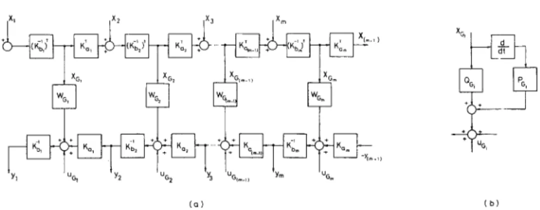
w h e r e -Y(m+l) represents the load through variables. The recursive relations can be displayed as a block diagram (see Figure 4a). Furthermore, the blocks Woj =

Po~(d/dt)

+ Qc. can be replaced by the detailed blocks in Figure 4b. Due to the presence of the derivaJtive operator blocks

(d/dt),

computations of

(d/dO xqi

are also required. These ex- pressions can be derived from equation (40) where the derivatives of the matrices

(K~I) r,

(K~l)r(Ka(.

x)) T will appear which may again be replaced by simpler forms by the use of the relatioh-obtained in A. 12 of the appendix of [1]; i.e.,

(d/dOR

= f i r - Rfl, where the second term may be omitted due to the multiplication of this expression by w.

XG,

X •

G~m'~ [~[ m-, m Gt

~

m IG m XG~ IGj (a) (b)

Figure 4. (a) Block diagram corresponding to forward recursive kinematic and inverse recursive dynamics equations in (40) and (41), respectively.

(b) Replacement of WGj block by an equivalent block diagram.

3. Example

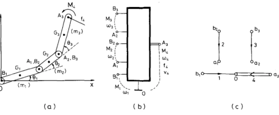
As an application of the closed form equations (20), the three-link plane manipulator with revolute joints is considered (see Figure 5a). All the rotation axes at the joints are along the z - axis, normal to the paper surface [17]. It is assumed that the links are homogeneous and prismatic in shape so that the centers of gravity occur at the mid points of the links. The lengths of the links are la, 12 and 13, respectively. At the firsst three joints the ter- minal velocities vl, v2, v3 are zero and the angular velocities r 1, 6o2, 6o3 have only z - components, 601,602, c03, respectively. We are also interested in only the z components of the torques M1, M2, M3 at the joints, indicated by M1, ME, M3, respectively. The manipulator is subject to the loads, f4 and M4, at the terminal A 3 (the z component o f ~ is zero while M4 has only a z - component, M4). Under these conditions, the manipulator as a four-port (scalar six-port) component with the schematic diagram and the terminal graph given in Figures 5b and 5c will have the following terminal equations which can be deduced directly from (20)

M1 M2 M3 V4x Vay 604 ')/11 "Y21 ")'31 ~ 1 1 ~ 1 2 ~13 ')'12 "Y13 I --~11 --~12 --~13 ")'22 "I"23 [ --~21 - ~ 2 2 - ~ 2 3 7 3 2 "Y33 ] --~31 --~32 - ~ 3 3 62t 6 3 1 1 0 0 0 ~22 ~32 I 0 0 0 ~23 ~33 [ 0 0 0 60 3 ______ -[- - - - - o _ 0 _1 (42)

NETWORK MODEL APPROACH TO THE ANALYSIS OF MULTIRIGID-BODY SYSTEMS 121 M4 y 0 3 / / / _ A1 ,B (m~) [3 3 M3 { ~3 ',, b2 B 2 ~ : = p A 3 2 M2( 11,4 4 G)2t~ I I (04 a~ ~ - I f~ ~ B,o5- I v~ b,o u31 0

t!i

o 4 ( a ) ( b ) ( c )

Figure 5. (a) A three-link plane manipulator.

(b) Pictorial diagram of the manipulator as the four-port mechanical component.

(c) The terminal graph of the manipulator (port 4 represents both the translational and rotational ter- minal variables).

where the scalar entries 7pq, ~ q and ~p are the r e d u c e d forms of the 3 x 3 submatrices o f W = SrWc, S, (K'S) and S'uG in equation (20), respectively. To obtain these reduced forms, in the case o f spherical joints, we should consider only the last rows and columns o f the submatrices o f equation (2):

E :1

E ~ 0

1

J% = * * , Rp,aj = 0 0 -(rp,@x 9 * J: -(re,@y (rp,@x 0

I~

1 I~

I~

Rq,Gj = 0 0 ( )x ~Gj 0 = -- (rq'GJ)r --(rq'G: )x rq~j , = ~OjO 0 ' g 0 g (43) where we define d q/pq = Cpq ~ Jr" dpq

and where the coefficients are obtained from equations (30) and (32) as

3

C?q = ~j=~ {Jj + mj[(rp,aj)x(rq,@x + (rp,@y(rq,@y]} (or = m a x ( p , q))

and

(44)

where the dot indicates the time derivative. The entries ~pq in equation (42) will be ob- tained from equation (36). Since

=

i0 0 1 i 00j

0

0

- r ~

, I =

1 0

- r ~ y r ~

0

0 1

the first two and the last rows and columns of equation (35) yield I(311 ~21 ~31 7

F --(rly +

r2y -I-

F3y )

--(F2y +

r3y ) --F3y

612 6Z2 b32 ~ = ~

(rlx + r2x + r3x)

(r2x + r3x)

r3x

613 (~23 r

1 1 1

(46) Finally, from the last rows of equations (33) and (34) we obtain

ml(rl,G1)x + m2(rl,G2)x + m3(rl,G3)x 1

= g

m2(r2,Gz)x + m3(r2,G3)x

.

(47)

m3(r3,G3)x

More explicit expressions for the entries

Cpq,

dpq, ~pq and/3p can be obtained by using the parameters indicated in Figure 5a. Note that for the links, we have Jy =

(1/12)mjl~ (j =

1, 2, 3). Let C i = cosOi, S i = sinOi, Cij = cos(Oi + Oj), Sij = sin(O i -]- Oj), Cij k -- cos(• i

+ Oj + Ok) and Sijk = sin(Oi + Oj + Ok),

then all the entries calculated from equations (44)-(47) are given in Table 1.

For a two-link manipulator with no loads, the terminal equations (42) take the following form

E M1

[ 1, 21

E ll I :l

48,

where the entries

"ypq

~-- Cpq

(d/dt) + dpq,/3p

can be obtained from Table 1 with m3 replaced by zero. These coefficients are given in Table 2.

4. Conclusions

Although the procedure presented in this article is only applied to obtain the terminal equa- tions (20) for a system of m rigid bodies connected in a special form, it is general. It can be applied to other rigid body systems having an arbitrary interconnection pattern which may exhibit an open or closed kinematic chain. Indeed, in the general case, the only change that occurs is in writing the fundamental circuit and fundamental cut-set equations obtained directly from the system graph representing the interconnection pattern of the rigid bodies.

N E T W O R K M O D E L A P P R O A C H T O T H E A N A L Y S I S O F M U L T I R I G I D - B O D Y S Y S T E M S 123 Table 1. Cll = ml(l/31~) + m2(l ~ + lll2C 2 + ~I~) + m3(l~ + 122 + 1/312 + 21112C 2 + 1213C 3 + 1113C23 ) c12 = c2~ = m 2 ( ~ t ~ + 8 9 z) + m3(l~ + 1At~ + 1213C 3 + l~t2C 2 + V2t113C23 c13 = c31 = m 3 ( ~ l ~ + 1/21213C3 + 1/21113C23) c22 = m2(%12) + m3(1Al ~ + l~ + 1213C3) c23 = c32 = m3(1/al 2 + 1/21213C3) c33 = m3(1/3l z) dtt = --rrb2(V2ltl2Szw2) -- m31l12SzoJ2 + 89 2 + w 3) dl2 = -m21AlllzS2(% + ~ - m3Vz1213S3~ - m31112Sz(~ + ~~ + V21l13S23(~ + ~2 + ~ 613 = -m3(1/2121383 + 1/21113823)(o~ 1 + 602 + 603)

d21 = m2(1/21112S20Ol) + m3(lllzS 2 q- 1/21113S23)o01 - 1/21213S3oo 3

d22 = -m3(1/21213S3oo3) d23 = -m3(1/ZlE13S3)(~ + ~ + ~3) d31 = m31/21113S23oo I + 1/21213S3(001 + W 2) d32 = -m3(1/21213C3)(oo I -b 6o2) , d33 = 0 till = -(11S1 + 12S12 q- 13S123), t~21 = -(12S12 + 13S123), ~31 = -/3S123 t~12 = llC1 + 12C12 q- 13C123 , t~22 = 12C12 "}- 13C123, ~32 = 13C123 ~13 = (~23 = (~33 = 1 a n d (1/g)fl I = m1(1/2llC1) + m2(llC 1 -b 1,~12C12 ) -b m3(11C 1 + 12C12 + 1/213C123) (1/g)/~ 2 : 1qb2(1/212C12) + m3(12C12 q- 1/212C123) (1/g)fl 3 = m3(1/213C123) Table 2. Cll c12 6"22 d l l d12 d21 d = 31 &

= ml(~Al~) + m2(l~ + lal2C 2 + 1Al22)

= c21 = m2(%l 2 + 1/21112C2) = m2(V3122) = -~(VzlllaS2~o2) = -m2[ 89 -1- w2) ] = m2(V21112S2Wl) = 0 = mlg(V211C1) + m2g(llC 1 + 1/212C12) = m2g(Vzl2C12 ) I f l 1 = l 2 = l t h e n t h e s e e q u a t i o n s r e d u c e to t h o s e g i v e n i n [17] o n p a g e s 102, 124 a n d 142.

Appendix

The explicit expressions of the submatrices appearing in the terminal equations (5) and (6) are given, respectively, in the following:

and with and and with

E'~

g~ 1 =

R r

I

Gbj

E ~

~ I' o]

gAJ= gbT1gaJ =

RGITbj I

RGa: I

=

Rj I

d +o.~

WBj ~-- gbj 1 WGj (Kb~.l) T = PBj

E m~, m~.o~I.O.:Eo m. Oo~"o~ 1

PB: =

mj Rarbj

JB~

0

~2G JB~

JB i = JGj + mj R ~ j R~bj

In: 1

uBj = Kb-~ 1 uGj = --

mj RGb: g

g-1 p. I I

0 I gA-f. 1 = I IT 0 ]

aj

gGa j I

'

Rj

d +QA:

w.~ = Ka-;. 1 . % r

~ = %

E

mj I mj R %

]

, QA~ =

E ~176

0 P a J =

mj R~, 9

Jaj

~2Gj Jaj

= K _ 1

[

m j g

]

UAj

aj UGi = --

mj R~a i g

(49)

NETWORK MODEL APPROACH TO THE ANALYSIS OF MULTIRIGID-BODY SYSTEMS 125

References

1. Y. Tokad, "A Network Model for Rigid Body Motion," Dynamics and Control, vol. 2, no. 1, pp. 59-82, 1992. 2. H.E. Koenig, Y. Tokad, and H.K. Kesavan, Analysis of Discrete Physical Systems, McGraw-Hilh New

York, 1967.

3. Y. Tokad, "On the Existence of Mathematical Models of Multi-terminal Linear Lumped Time Invariant Networks," Proc. of the (1981) European Conference on Circuit Theory and Design (ECCTD'81), pp. 886-891, The Hague, The Netherlands, 1981.

4. Y. Tokad, "On the Topological Conditions for Linear Lumped Time Invariant Networks Containing Multi- terminal Components," Bulletin of the Technical University oflstanbul, vol. 40, no. 2, pp. 479-496, 1987. 5. K. Abdullah and Y. Tokad, "On the Existence of Mathematical Models for Multiterrninal RCF Networks,"

IEEE Trans. Circuit Theory, vol. CT-19, no. 5 pp. 419-424, 1972.

6. P.R. Bryant and J. Tow, "The A-Matrix of Linear Passive Reciprocal Networks," J. Franklin Inst., vol. 293, no. 6 pp. 401-419, 1972.

7. A. Recski, Matroid Theory and Its Applications, Springer-Verlag: Budapest, 1989.

8. S. Seshu and M.B. Reed, Linear Graphs and Electrical Networks, Addison-Wesley Publishing Co., Inc., MA, 1961.

9. M. Vukobratovic and V. Potkonjak, Dynamics of Manipulation Robots (Scientific Fundamentals of Robotics; 1), Springer-Verlag: Berlin, Heidelberg, 1982.

10. J.Luh, M. Walker, and R. Paul, "On-line Computational Scheme for Mechanical Manipulators," J. Dynamic Systems, Measurements, and Control, vol. 102, no. 6, pp. 69-76, 1980.

11. J.M. Hollerbach, " A Recursive Lagrangian Form~ation of Manipulator Dynamics and Comparative Study of Dynamic Formulation Complexity," 1EEE Trans. Syst., Man, Cybern., vol. SMC-10, no. 11, pp. 730-736, 1980.

12. M.W. Walker and D.E. Orin, "Efficient Dynamic Computer Simulation of Robotic Mechanism," J. Dynamic Systems, Measurement, and Control, vol. 104, pp. no. 9, 205-211, 1982.

13. L.T. Wang and B. Ravanl, "Recursive Computations of Kinematic and Dynamic Equations for Mechanical Manipulators," 1EEE Journal of Robotics and Automation, vol. RA-1, no. 3, pp. 124-131, 1985. 14. R. Nigam and C.S.G. Lee, " A Microprocessor-Based Controller for the Control of Mechanical Manipulators,"

IEEE Journal of Robotics and Automation, vol. RA-1, no. 4, pp. 173-182, 1985.

15. J.M. Hollerbach and K.C. Suh, "Redundancy Resolution of Manipulators Through Torque Optimization," 1EEE Journal of Robotics and Automation, vol. RA-3, no. 4, pp. 308-316, 1987.

16. R.P. Paul, Robot Manipulators: Mathematics, Programming, and Control, The MIT Press: Cambridge, Massachusetts, 1981.