Controlled dephasing in single-dot Aharonov-Bohm interferometers
V. Moldoveanu and M. ŢoleaNational Institute of Materials Physics, P.O. Box MG-7, Bucharest-Magurele, Romania
B. Tanatar
Department of Physics, Bilkent University, Bilkent, 06800 Ankara, Turkey
共Received 3 April 2006; revised manuscript received 14 September 2006; published 8 January 2007兲
We study the Fano effect and the visibility of the Aharonov-Bohm oscillations for a mesoscopic interfer-ometer with an embedded quantum dot in the presence of a nearby second dot. When the electron-electron interaction between the two dots is considered the nearby dot acts as a charge detector. We compute the currents through the interferometer and detector within the Keldysh formalism and the self-energy of the nonequilibrium Green’s functions is found up to the second order in the interaction strength. The current formula contains a correction to the Landauer-Büttiker formula. Its contribution to transport and dephasing is discussed. As the bias applied on the detector is increased, the amplitude of both the Fano resonance and Aharonov-Bohm oscillations are considerably reduced due to controlled dephasing. This result is explained by analyzing the behavior of the imaginary part of the interaction self-energy as a function of energy and bias. We emphasize as well the role of the ring-dot coupling. Our theoretical results are consistent with the experimental observation of Buks et al.关Nature 391, 871 共1998兲兴.
DOI:10.1103/PhysRevB.75.045309 PACS number共s兲: 73.23.Hk, 85.35.Ds, 85.35.Be, 73.21.La
I. INTRODUCTION
The coherent nature of electronic transport through Aharonov-Bohm rings with embedded quantum dots 共QD兲 was clearly established in various experiments.1–4In particu-lar the periodic Aharonov-Bohm oscillations 共ABO兲 of the interferometer conductance and the mesoscopic Fano effect were systematically observed and are nowadays well under-stood theoretically, at least for noninteracting dots or within mean-field approaches.5–12 A more subtle problem in elec-tronic interferometry is related to the decoherence effects caused by inelastic processes like electron-electron interac-tion, electron-phonon or electron-photon coupling. More generally共see Refs.13and14兲 the decoherence appears due to the mutual interaction between a coherent system and its environment and leads to a loss of quantum interference be-tween different electronic trajectories.
A particular type of decoherence is the so-called con-trolled dephasing introduced by Gurvitz15 for a double dot system. Using one of the dots as a charge detector Gurvitz proved that the off-diagonal elements of the reduced density matrix of the measured dot are damped. Otherwise stated, the dot coherence is destroyed during the measurement process. Following this idea Buks et al.16 have patterned an Aharonov-Bohm interferometer共ABI兲 with a quantum point contact 共QPC兲 located near the quantum dot. The two sub-systems were not coupled directly so their mutual coupling comes only from the Coulomb interaction between electrons in the dot and in QPC. It was found that the transmission through the latter TQPC increases smoothly as the plunger gate potential Vg applied on the dot increases. Also,
when-ever a resonant conductance peak of the quantum dot is be-ing scanned the QPC “feels” the passbe-ing of a charge carrier through the dot and is therefore called “which path detector” 共WPD兲. Conversely, the current flowing through the WPD induces a reduction of the Aharonov-Bohm oscillations in the ring when the detector is subjected to a rather large bias.
At small bias instead the visibility of the oscillations is not affected by dephasing. A similar experiment with coupled quantum dots was performed by Sprinzak et al.17 with a double quantum dot.
The first theoretical consideration of measurement dephasing in quantum dots coupled to nearby detectors was given by Aleiner et al.18The dephasing rate共i.e., the inverse of the time tdrequired for the detection of addition processes
in the QD兲 was computed for weak mixing between the scat-tering states describing the WPD. A similar result was ob-tained by Levinson for a single-level isolated QD coupled to a conducting WPD共Ref. 19兲 using the influence functional method.20 Another treatment proposed by Hackenbroich7 is based on the master equation techniques. The reduced den-sity matrix of an isolated quantum dot coupled to a WPD is shown to have modified off-diagonal elements and the dephasing rate was computed within the Markov approxima-tion, taking into account the phase change of the QPC S matrix when one electron enters the QD.
An alternative view on dephasing in Coulomb-coupled mesoscopic conductors was developed by Büttiker et al.21 The electron-electron interaction is described by geometrical capacitances and the dephasing rate is given in terms of the voltage fluctuations in QD and WPD.
In a recent work Silva and Levit22 presented a detailed analysis of the dephasing rate for a quantum dot perturbed by a WPD by computing the interaction self-energy up to the second order in the Coulomb coupling constant. In the zero temperature limit the dependence of the dephasing rate on the ratio eV /⌫ 共eV being the bias applied to the detector and ⌫ the lead coupling兲 was discussed. Moreover, in a recent work23 it has been found that the dephasing rate of a quan-tum dot coupled to a detector is maximum at the resonance of the latter.
Although the experiment of Buks et al. has triggered im-portant theoretical developments the main issue of the con-tributions we just mentioned has been the calculation of the
dephasing rate for a quantum dot which is isolated or coupled to two leads rather than embedded in a ring. The magnetic field is also absent and, to our best knowledge, no theoretical investigation of dephasing in the specific geom-etry of Ref.16was performed.
Consequently an analysis of the Aharonov-Bohm oscilla-tions depending on the interaction strength or on the WPD bias is not available. Moreover, the recent observation of the mesoscopic Fano effect in single-dot ABI 共Ref. 4兲 poses naturally the problem of possible dephasing effects on the Fano interference.
In this work we consider an Aharonov-Bohm interferom-eter with an embedded dot which is coupled via a Coulomb term to a second dot playing the role of WPD. We take into account the geometry of the whole system 共ring+dot + detector兲 and compute the currents through the interferom-eter and WPD within the Keldysh formalism. In particular the interferometer is a many-level system and therefore the current formula is not as simple as for a single-site dot. Fol-lowing Ref.22, we compute the first two contributions to the interaction proper self-energies. Our calculations present clear plots showing the effect of dephasing on the mesos-copic Fano line. We capture as well the suppression of the AB oscillations when a large bias is applied to the detector and discuss the conditions required for the observation of the controlled dephasing. We mention here that in a recent paper24Szafran and Peeters presented an interesting effect in a two dimensional noninteracting ring without any quantum dot. It was shown that due to the Lorentz force the current is asymmetrically injected and that the Aharonov-Bohm oscil-lations are also affected.
Let us discuss now the approximations we have used in the calculations. A full treatment of the electron-electron in-teraction would require one to take into account as well the intradot Coulomb interaction and the spin degree of freedom. We argue below that in the absence of the spin-flip effects and in the regime of weak ring-dot the intradot interaction does not bring new effects that have not been addressed be-fore in the existing literature. In a recent paper Jiang et al.25 claimed that the intradot interaction does not lead to dephas-ing while König and Gefen26predicted that the spin-flip pro-cesses are responsible for the observed asymmetry of the Aharonov-Bohm oscillations.27 The conditions for which a spin pair state is entangled in the dot are rather unlikely to meet in experiments and the data provided by Buks et al. do not reflect such a contribution to dephasing. Another situa-tion in which the intradot interacsitua-tion and the spin degree of freedom can lead to interesting features is the Kondo regime of the embedded dot共see Ref.28 for experimental results兲. This problem was studied by Silva and Gefen,29 the main result being that the Kondo correlations reduce the decoher-ence, as the transport in this case is due to spin fluctuations which are not detected by the charge detector. Further theo-retical investigation of the decoherence in the Kondo regime was reported in Ref.30. However, in the experimental setup of Buks et al. the weak ring-dot coupling prevents the for-mation of the Kondo correlated state and therefore we be-lieve that neglecting this mechanism is permitted.
The outline of the paper is as follows. Section II settles the notation and gives the relevant formulas for currents and
self-energies. Section III presents the numerical results and their discussion. We conclude in Sec. IV.
II. THE MODEL AND THE CURRENT FORMULA A. The current formula
We describe our system by a tight-binding Hamiltonian and consider in a two-lead geometry a simple interferometer composed of three sites, one of them simulating the quantum dot. The “which path detector” is a single site coupled also to two leads 共see Fig. 1 for geometry and notation兲. The full Hamiltonian reads:
H共t兲 = H0+共t兲共Hi+ Ht兲, 共1兲
H0= HI+ HD+ HL, 共2兲
where the unperturbed Hamiltonian H0 contains the Hamil-tonians of the interferometer I, detector D, and leads L. The last two terms in Eq.共1兲 describe the interferometer-detector interaction and their coupling to the leads. The two perturba-tions are adiabatically applied, more precisely the switching function 共t兲 is defined such that 共t兲=et for t⬍0 and
共t兲=1 for t⬎0.is a small positive adiabatic parameter.
The adiabatic switching of both the lead-system coupling and interaction eliminates the complications due to the Mat-subara complex time contour which would otherwise appear in the perturbation theory for the Keldysh-Green functions.31,32Physically this procedure means that the initial correlations are not taken into account.32The explicit form of the Hamiltonians are as follows:
HI=
兺
i=1 3 共i+␦i2Vg兲di†di+兺
i⫽j,i,j=1 3 eiijt ijdi†dj, 共3兲 HD=4d4 † d4, Hi= Ud2 † d2d4 † d4, 共4兲 HL=兺
兺
n=0 ⬁ 关ncn † cn+ tL共cn † c共n+1兲+ H.c.兲兴, 共5兲 Ht= tLI共d1†c0␣+ d3†c0兲 + tLD共d4†c0␥+ d4†c0␦兲 + H.c., 共6兲 di, di†are annihilation/creation operators in the interferometer 共i=1,2,3兲 and detector 共i=4兲. Similarly we have on leads the pair c, c†. In the leads’ Hamiltonian HL, is the lead
index共i.e.,=␣,,␥,␦兲 and the parameter tLis the hopping
FIG. 1. The interferometer-detector system. The quantum dot is described by site 2 which is Coulomb-coupled to the single-site detector 4.
constant on leads. In Eq. 共3兲 Vg simulates the gate voltage
applied on the dot and the magnetic fluxpiercing the ring is included in the Peierls phases ij attached the hopping
constants tij. It is expressed in quantum flux units 0 and specifically we have12=23=31= 2/ 30 and ji=*ji.
Hidescribes the Coulomb interaction of strength U between
the embedded dot and the detector. Ht couples the
interfer-ometer and the detector to the sites 0 of the lead . The corresponding hopping constants are tLIand tLD. Assuming
that a steady-state regime is already achieved at time t, the nonequilibrium Green’s function formalism gives the current through the lead␣ 共see for example Ref.33兲
具J␣典 =etLIប
冕
−⬁⬁
dE Re G1␣⬍共E兲, 共7兲
where G1␣⬍共E兲 is the Fourier transform of the real-time lesser Green’s function:
G1␣⬍共t,t
⬘
兲 = i具c0␣,H† 共t⬘
兲d1,H共t兲典. 共8兲 In the above equation 具·典 denotes the statistical average on the fermionic Fock space with respect to the density matrix operator of the unperturbed time-independent HamiltonianH0. The operators are written in Heisenberg picture with re-spect to H共t兲. It is well known that the calculation of G1␣⬍ requires the knowledge of the Green-Keldysh function de-fined as follows:
Gmn共,
⬘
兲 ª − i具TC„dm,H共兲cn,H† 共
⬘
兲…典, 共9兲 where TCis the time-ordering operator along theSchwinger-Keldysh “contour” C =共−⬁,max兵,
⬘
其兴艛关max兵,⬘
其,−⬁兲. The first step of the calculation is to express the mixed-indices Green function G1,0␣ using its Dyson equation 共see Ref.35兲. Since the lead␣is coupled to the interferometer by a single site we have:G1␣共,
⬘
兲 = tLI冕
Cd1G11共,1兲g0␣,0␣共1,
⬘
兲, 共10兲 where g0,0is the Green’s function of the semi-infinite lead=␣,,␥,␦ at site 0. This quantity is known共see Ref.33兲:
g0,0R 共E兲 =
冦
1 2tL 2共E − i冑
4tL 2 − E2兲 if E ⬍ 兩2tL兩, 1 2tL 2共E −冑
E2− 4tL2兲 if E ⬎ 兩2tL兩冧
共11兲in which tLis the hopping constant on leads. Also one has:
g0,0⬍ 共E兲 = 2if共E兲共E兲 = − 2if共E兲Im g0,0R 共E兲. 共12兲
Here f共E兲 is the Fermi function for the lead and is the electronic density at the site 0 of the lead. Note that since we take the same hopping constant on leads does not de-pend on. Expressing the contour integral in Eq.共10兲 via the Langreth rules34and plugging its Fourier transform into Eq. 共7兲 one gets after simple calculations the following current formula 共we shall omit the energy dependence when this causes no confusion兲: 具J␣典 = − etLI2 ប
冕
dEIm共2G11 R f␣+ G11⬍兲. 共13兲 Note that due to the leads’ density of states 关see Eq. 共12兲兴 the integral runs only over the continuous spectrum of the leads 关−2tl, 2tL兴. The current formula Eq. 共13兲 reduces theproblem to the calculation of a matrix element of the inter-ferometer Green’s function. This can be done using the Feynman-Dyson expansion along the contour C. Without giving the straightforward details we state that the contour Green’s function which is a 4⫻4 matrix satisfies the equa-tion:
G = Geff+ Geff⌺iG, 共14兲
where⌺iis the self-energy due to interaction and the
effec-tive Green function describes the noninteracting system in the presence of the leads, i.e.,
Geff= G0+ G0⌺lGeff. 共15兲 Here G0 describes the noninteracting decoupled system 共QD+QPC兲 and ⌺lis the usual self-energy of the leads:
⌺l,mn共z兲 =
冦
tL2g0,0共z兲 if m = n = 1,3, tL 2 „g0␥,0␥共z兲 + g0␦,0␦共z兲… m = n = 4, 0 if m⫽ n or m = n = 2.冧
共16兲 B. The self-energiesIn what concerns the interaction self-energy⌺i we
com-pute only the first two contributions⌺i1and⌺i2which can be
identified from the diagrams in Fig.2. We used double lines for electronic propagators since they are “dressed” by the leads’ self energy. Using the Langreth rules for dealing with time-integrals and performing the Fourier transform one ob-tains for m , n = 1 , 2 , 3, ⌺i,mnR,1共E兲 = −␦m2␦n2i U 2
冕
dE⬘
Geff,44 ⬍ 共E⬘
兲, ⌺ i,mn ⬍,1共E兲 = 0, 共17兲 ⌺i,mn⬍,2共E兲 =␦m2␦n2 U2 22冕
dE1dE2Geff,22 ⬍ 共E − E 1兲 ⫻Geff,44⬍ 共E2兲Geff,44⬎ 共E2− E1兲. 共18兲 The explicit forms for⌺i,44R,1,⌺i,44R,2, and⌺i,44R,⬍ are similar, theFIG. 2. The first two contributions to self-energy⌺i1共left兲 and ⌺i
only difference being that Geff,22and Geff,44have to be inter-changed. The retarded self-energy is related to the lesser and greater self-energies by the identity共see Ref. 22兲:
⌺i R,2共E兲 = lim ⑀→0+ i 2
冕
dE⬘
⌺i⬎,2共E⬘
兲 − ⌺i⬍,2共E兲 E − E⬘
+ i⑀ . 共19兲 To obtain the greater self-energy⌺i,mn⬎,2 one has just to inter-change⬎ and ⬍. The Dyson and Keldysh equations for the retarded and lesser Green’s functions read:GR= GeffR + GeffR⌺i R GR, 共20兲 G⬍=共1 + GR⌺i R兲G eff ⬍共1 + ⌺ i A GA兲 + GR⌺i⬍G A , 共21兲
Geff⬍ = GeffR⌺l⬍Geff
A
. 共22兲
The last identity uses that共G0R兲−1G 0
⬍= 0. A simple calculation gives alternative forms of共14兲 and 共21兲:
G = G0+ G0共⌺l+⌺i兲G, 共23兲
G⬍= GR共⌺l⬍+⌺i⬍兲G A
. 共24兲
In the following we shall use the perturbative results from above to compute the current 具J␣典 via Eq. 共13兲. Using the identity GR− GA= 2iGRIm⌺RGA, Eq. 共24兲 and the explicit expression for ⌺l,11 and ⌺l,33, a straightforward algebra
gives: 具J␣典 =etLI 2 ប
冕
−2tL 2tL dE共22G13RG31A共f␣− f兲 −G12R Im共2⌺i,22R f␣+⌺i,22⬍ 兲G21A兲 ª J1+ J2. 共25兲 The first term J1 from Eq. 共25兲 is clearly a Landauer-type current. The second term in the current formula is a correc-tion to the Landauer formula due to interaccorrec-tion and was not considered in previous papers.18,22Equation共25兲 is a central result of the present work. In the following we provide fur-ther supporting arguments for its validity.As emphasized in the seminal paper of Meir and Wingreen36 the Landauer formula holds also for interacting systems in linear regime at zero temperature. The argument is based on the general result of Luttinger37 according to which the imaginary part of the self energy vanishes at the Fermi level, in all orders of the perturbation theory. The subtle point here is that if one of the two interacting sub-systems 共i.e., the detector兲 is submitted to a finite bias one gets a nonvanishing imaginary part of the self energy even in the limit T→0. The explicit calculation in Ref. 22 for the case of a single-site dot coupled to a quantum point contact clearly shows this fact. As we shall see in Sec. III the cor-rection to the Landauer formula contributes nontrivially to transport and therefore should be kept in the current formula. As a consequence, the total current cannot be expressed in terms of the QD transmittance. We point out that in Ref.22 the starting point is a non-interacting formula for the QD transmittance tQD which involves only the retarded Green’s function. The latter in turn contains the self-energies due to both e-e interactions and lead-dot coupling. However, König and Gefen26 argued recently that such a formula may not
properly define the transmission amplitude of interacting quantum dots. In spite of the fact that even in the interacting case the integrand of J1 resembles a transmission amplitude the presence of the correction due to the Im⌺R and Im⌺⬍ prevents one to define safely tQD. The rest of the paper will be mainly devoted to the analysis of J1 and J2.
The current through the lead ␥ is obtained in a similar way. We do not give its expression here but we note that the first order self-energy felt by the detector ⌺i,44R,1 = −2i U兰dEGeff,22⬍ 共E兲=U具n22典 where 具n22典 is the electronic occupation number of the noninteracting dot. Then clearly the WPD Green functions record the sudden change of具n22典 by one, corresponding to addition of one electron to⫹ the QD.
Although the self-energy expressions are not simple the calculations can be eventually performed since the effective lesser Green functions are given in Eq.共22兲 and the retarded functions can be computed since they describe noninteract-ing systems 共m,n=1,2,3兲. Then clearly, one has to invert finite rank non-hermitian matrices and perform the energy integrals from Eqs.共17兲–共19兲 to get the self-energies expres-sion. After some straightforward calculations the retarded self-energy of the dot reads:
⌺i,22R,2共E兲 = i 2tLD 4 U2
冕
dE⬘
dE⬙
˜ 44共E⬙
兲冉
Geff,22⬎ 共− E⬘
兲 E + E⬘
− E⬙
+ i␦ − Geff,22 ⬍ 共E⬘
兲 E − E⬘
+ E⬙
+ i␦冊
, where the generalized spectral density:
˜44共E兲 ª
兺
,⬘=␥,␦
冕
dE1dE2␦共E1− E2− E兲共E1兲共E2兲f⬘共E2兲 ⫻„1 − f共E 1兲…兩Geff,44 R 共E 1兲兩2兩Geff,44 R 共E 2兲兩2. 共26兲 This result is similar to Eq. 15 from Ref. 22 We have however extra terms coming from the more complex geom-etry and the spectral density˜44is far more complicated than the one given in Eq.16 from Ref.22. Now one should use Eq.共22兲 to express the effective Green’s functions. Explicit expressions for the imaginary and real parts of ⌺i,22R,2 are found by virtue of the principal-value formula. One can show without much effort that in the zero temperature limit Im⌺i,22R,2共E兲=0 if there is no bias applied on the WPD 共i.e.,
␦=␥兲. Thus, there will be no dephasing as long as the detector is in equilibrium.
At this level of approximation the retarded Green’s func-tion of the interferometer is known from the Dyson equafunc-tion once we have computed all the effective Green’s functions and the first two contributions to interaction self-energy. It is now a usual Green’s function associated with a single par-ticle operator G44R共E兲 = 具4兩共HD−⌸D共⌺l R +⌺i R兲⌸ D− E兲−1兩4典, 共27兲 Gmn R 共E兲 = 具m兩共H I−⌸I共⌺l R +⌺i R兲⌸ I− E兲−1兩n典, 共28兲
where⌸D,⌸I are projection operators onto their associated
and⌸I=兺i=1
3 兩i典具i兩. Also, the self-energies are now associated with the operators ⌺共E兲ª兺i,j=14 ⌺ij共E兲兩i典具j兩. Then following
the same steps as in Refs.11 and12we use the Feschbach formula to rewrite Gmn
R
in a more useful form:
Gmn R 共z兲 = 具m兩G R R共z兲 + H RDGD R共z兲H DR兩n典, 共29兲
where HRDand HDR are transfer terms between the dot and
the ring 共i.e., HRD= t12ei12兩1典具2兩+t32ei32兩3典具2兩兲 and GR R
= (HR−⌸I⌺l R共z兲⌸
I− z)−1describes the ring without the dot in
the presence of the two leads␣,. GDis the effective Green
function of the dot共Hdis the single-particle Hamiltonian of
the noninteracting uncoupled dot兲:
GD R 共z兲 = „Hd−⌸I⌺i R共z兲⌸ I−⌺d共z兲 − z…−1, 共30兲 where⌺dªHDRGR R共z兲H
RDis a noninteracting effective
self-energy due to the ring-dot coupling. Obviously, this quantity does not depend on bias and can be computed explicitly by writing the 2⫻2 matrix GRR. We shall need⌺d in our
calcu-lations presented in Sec. III. The advantage of having GRin this form is twofold. First, the interaction self-energy appears naturally only in the dot’s Green’s function. Second, the resonant processes involving the dot are collected in the sec-ond term and clearly separated from the noninteracting co-herent background contribution of the reference arm of the interferometer.
III. RESULTS AND DISCUSSION
Let us first set some notation for the parameters that will be used throughout this section. We work always with a weak ring-dot coupling and put t12= t23ªtRD. The leads are
instead strongly coupled to the detector and interferometer. As the energy unit we choose the hopping constant on leads
tL. Consequently the gate potential, the energy, self-energies,
and the bias are to be understood in tLunits while the current
will be given in etL/ h units. The results do not depend on the
value of tL so we choose for simplicity tL= 1. The on-site
energy of the leads is chosen as the energy reference. The bias on the interferometer is denoted by V0 and the bias on the detector by V. We apply both biases in a symmetric way. More precisely, the chemical potentials of the unbiased leads attached to the interferometer and detector are shifted by ±V / 2 and ±V0/ 2, respectively.
Before investigating the effect of the electron-electron in-teraction on the AB oscillations let us look at the Fano line shapes of the current J␣. Figure3shows the behavior of the Fano resonance when the bias V on the detector increases, for two values of the interaction strength U = 0.3 and U = 0.5. The magnetic flux is fixed at = 0.0 and the bias V0 = 0.1. Other parameters are given in the figure caption. There are two features to observe:共i兲 the amplitude of the Fano line decreases for larger bias and共ii兲 when U=0.5 the Fano line is shifted with respect to the resonance at U = 0.3. The reduc-tion of the Fano line is more pronounced for U = 0.5. The inset in Fig.3 gives the current J␥through the detector as a function of the gate potential Vg applied on the dot at
inter-action U = 0.5. We take the on-site energies i= 0 for i
= 1 , 2 , 3 and4= 0.1. Clearly the detector feels the electrons
passing through the embedded dot. The height of the current step is a measure of the detector sensitivity to the electrons crossing the embedded dot. The inset shows that as the bias increases the response of the detector is enhanced. As we shall show below this suggests that the quantum interference within the interferometer is more affected by the electron-electron interaction at large bias. The current step does not follow precisely the Fano resonance for U = 0.5 because in our approximation the first order self-energy of the detector ⌺i,44
R,1 is computed in terms of the occupation number of the
noninteracting dot具n22典 共this quantity increases by one as the embedded dot accumulates one electron兲. For this reason the steplike behavior of J␥is correlated with the noninteracting Fano line which is located to the left of the interacting one. A better correspondence between the detector characteristics and the Fano line can be achieved within a self-consistent calculation. Here we prefer to keep the lowest approximation and look for the role of the second order self-energy in trans-port. We note also that the positions of the Fano line and of the jump in the detector signal are not strictly around the eigenvalue2of the isolated dot. As shown in Eq.共30兲 even in the noninteracting case the effective Green’s function of the embedded dot has a pole whose real part does not have to coincide with 2. This is due to the ring-dot coupling self-energy ⌺d which brings a shift in the real part of the
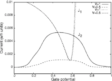
reso-nance共for more discussion of this point we refer to Ref.11兲. The two currents from Eq. 共25兲 are compared in Fig. 4 which is a zoom from the Fano dip shown in Fig. 3 at U = 0.3. The correction J2to the Landauer current J1takes sig-nificant values only around the Fano resonance. J1shows a dip structure depending very weakly on bias. In contrast, J2 increases with V and there is a critical bias Vcsuch that if
V⬎Vcthen J2⬎J1. The numerical calculations show there-fore that in the neighborhood of the Fano resonance J2 can-not be neglected and also that this correction is responsible for the enhanced Fano dip seen in Fig.3. This means that J2 diminishes the whole Fano line, hence it affects its visibility. The AB oscillations appear when the magnetic field varies and the gate potential is fixed to a value from the range
FIG. 3. Coulomb-modified Fano line shapes as a function of the gate potential Vg 共in units of tL兲 at different bias on the detector;
solid line V = 0.0, dashed line V = 0.5, dotted line V = 1.0. Inset: the detector response at U = 0.5. Other parameters: tRD= 0.3, tLD= 1,
where the Fano line develops. Figure5 shows the reduction of the AB oscillation amplitude as the bias on the detector V increases. In Fig.5共a兲we plot oscillations around the Fano peak共Vg= 0.55, U = 0.3兲 from Fig.3. The dephasing appears
already at small bias V = 0.25 and is considerably enhanced at large bias. At V = 1 the AB oscillation amplitude is reduced roughly by 50%. A slight asymmetry with respect to= 0 is noticed. Around the Fano peak the dephasing mainly affects the ABO maxima and is due to the reduction in the Landauer like current J1. Interestingly, the oscillations taken near the Fano dip Vg= 0.4关see Fig.5共b兲兴 are more damaged because
their minima are pushed upward. This is due to the increas-ing contribution of J2. In particular, around integer values of the magnetic flux the reduction of the maxima and minima are comparable. A similar dephasing effect is obtained for a gate potential associated with the middle of the Fano line
共not shown兲. The above observations show that both currents contain the dephasing effect due to electron-electron interac-tion and suggest that in order to detect experimentally the dephasing in such systems one should look around the Fano dip because here the effect is stronger. The double-maxima aspect of the AB oscillations in Fig.5共b兲is not an interaction effect and it is easy to explain. As known, the energy levels of the ring behave like sin. Single-maxima AB oscillations are obtained when the energy of the incident electron E is close to a ring level while the double oscillations appear when E crosses it twice in flux period共see examples in Ref. 38兲.
In the following we investigate the conditions under which the suppression of the AB oscillations due to the dot-detector interaction is discerned. To this end we compare the imaginary parts of the two self-energies appearing in the ef-fective Green’s function of the embedded dot关see Eq. 共30兲兴. Note that ⌺d appears only in the Landauer-like current and
that兺i,22R,1 is real. At low temperature and small bias applied on the interferometer the relevant range for this comparison is 共see the integration limits in the current formula兲 关 − eV0/ 2 ,+ eV0/ 2兴.
In Fig. 6 we give the imaginary parts of the two self-energies as a function of energy for different values of bias on the detector. The bias applied on the interferometer is
V0= 0.1 and the magnetic field is fixed at = 0. Im⌺d
de-pends only on the energy of the electrons entering the inter-ferometer while Im兺i,22R,2 is very sensitive to both bias V, and the chemical potential on leads . For = 0 it nearly van-ishes at energies smaller than −0.5 but increases as E ap-proaches the upper bound of the lead’s spectrum 2tL. A first
important observation is that in the integration domain 关−0.05,0.05兴 the imaginary parts of ⌺dand兺i,22R,2 are
compa-rable. Secondly, we remark that as the bias V increases Im兺i,22R,2 exceeds 共in absolute value兲 Im ⌺d. Then looking at
the AB oscillations from Fig.5one infers that the dephasing effect appears as the interaction self-energy is of the same
FIG. 4. The Landauer-like current J1 共dotted and dash-dotted
lines兲 and the correction J2共solid and long-dashed line兲 around the Fano dip. J1changes negligibly with increasing the bias V while J2
increases strongly and even exceeds J1at V = 1.0. The gate potential is given in tL units. Other parameters: tL= 1,=0.
FIG. 5. The reduction of the AB oscillations with increasing bias on the detector for two values of the gate potential共a兲 Vg= 0.55 and
共b兲 Vg= 0.40 共in tL units兲. From top to bottom the biases are V
= 0.00, V = 0.25, V = 0.50, V = 0.75, V = 1.00共in tL units兲. Other pa-rameters: tL= 1,=0.
FIG. 6. The imaginary part of the self-energies⌺i,22R,2and⌺das a
function of energy E for fixed bias V0= 0.1 and chemical potential . Im ⌺dis plotted with dashed line and depends only on energy. At
=0.0 two plots are shown for Im ⌺i,22
R,2: V = 1.0—full line and V
= 0.5 dashed-dotted line. For=1.0 the full line corresponds to V = 1.0. All quantities are given in tLunits and tL= 1.
order as the effective self-energy due to the ring-dot cou-pling. The stronger suppression of the AB oscillation at bias
V = 1 is also understood. We have checked that by varying
the magnetic flux the self-energies do not vary drastically and the above discussion still holds.
Another interesting aspect showing the controlled feature of dephasing is revealed when the bias window of the inter-ferometer is shifted by changing the equilibrium chemical potential of the decoupled leads. The left curve in Fig.6 gives again the function Im兺i,22R,2共E兲 at large bias V=1 but now for = 1. Thus, the integration domain is now 关0.95, 1.05兴 and in this region Im 兺i,22R,2ⰆIm ⌺d. We found in this
case that the dephasing is more difficult to notice. Actually the oscillations of the Fano peak for zero bias and V = 1 do not differ significantly and a very small dephasing appears when a gate potential around the Fano dip is chosen. There-fore, the dephasing is controlled not only by the bias applied on the environment but also by the properties of the dephased system, i.e., by the behavior of the self-energy⌺d
which depends in turn on the ring-dot coupling and on en-ergy. We stress that in Ref.22the leads’ self-energy does not depend on E and the above discussion cannot be made.
Evidently, one has to check whether the above results are still valid at other values for the bias across the interferom-eter. In Fig. 7共a兲 we show the Fano line shapes for three values of V0. The Coulomb interaction strength is chosen here as U = 0.5. As V0increases the Fano lines move globally to higher values of the current and are broader. This feature is easy to understand. The main point is that the width of the bias window sets the range of the gate potential for which one can observe the Fano effect. This is because the quantum interference is possible only as long as the discrete level of the embedded dot lies within the bias window. Therefore, at large bias the Fano line has a larger width due to a larger window. In Fig.7共b兲 we plot the AB oscillations taken from the Fano dip of the dotted line in Fig.7共a兲. As the bias on the detector increases from V = 0.25共full line兲 to V=0.50 共dashed line兲 the dephasing effect develops and is similar to previous plots.
In what concerns the role of the interaction strength it is clear that the dephasing is enhanced as U increases, since the
interaction self-energy is directly proportional to U2. On the other hand our perturbative approach does not allow large values for U. Since the embedded dot and the detector are spatially separated by approximately 1m we believe that this parameter has also small values in the concrete experi-mental realization. We also point that in the case where the dephasing is clearly observed 共i.e., when Im 兺i,22R,2⬃Im ⌺d兲
the interaction strength U = 0.3 is much bigger than Im⌺d.
Now, let us see what happens when the ring-dot coupling is varied. The analytical expression for⌺dshows that it
be-haves like tRD
2
. Thus, by keeping the bias fixed and decreas-ing tRD the imaginary part of ⌺d diminishes. Consequently
the ratio Im兺i,22R / Im⌺dincreases and from the above
analy-sis one expects further reduction of the AB oscillation. This is precisely demonstrated in Fig.8where AB oscillations at bias V = 0.5 are given for different couplings. Each oscillation corresponds to the peak of the Fano line at the given tRD.
Physically the enhanced dephasing noticed at smaller ring-dot couplings is understandable because by reducing tRD the
dwell time of electrons inside the dot increases and therefore they can be easily detected. We stress that in experiments the ring-dot coupling can be adjusted freely and therefore the
FIG. 7.共a兲 Fano lines at different values of the bias applied on the interferometer; full line—V0= 0.15, dashed line V0= 0.2, dotted line
V0= 0.25. 共b兲 The reduction of the Aharonov-Bohm oscillations at V0= 0.25. Vg= 0.52 corresponds to the Fano dip. Other parameters U = 0.5, tRD= 0.3, tLD= 1, tLI= 0.8,=0. All quantities are given in tLunits and tL= 1.
FIG. 8. The effect of the ring-dot coupling on the dephasing. As tRDdecreases the AB oscillations are more damaged. Other param-eters: U = 0.3, V0= 0.1, tLD= 1, tLI= 0.8.
dephasing in the system we consider should be easily seen for weak ring-dot couplings.
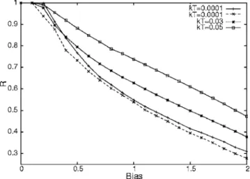
Further analysis of the controlled dephasing is contained in Fig.9. It gives the ratio R = A共Vi兲/A0 between the ampli-tude of the AB oscillations at different biases Vi and the
zero-bias amplitude A0. This quantity is somehow similar to the visibility of the oscillations measured in Ref.16. At small temperatures we give the visibility for two gate potentials corresponding to the Fano peak共full line兲 and dip 共dashed line兲. The behavior of R confirms that in the presence of mutual Coulomb interaction between the detector and dot the coherence of the interferometer is reduced as the bias in-creases. This was the main experimentally observed feature in the work of Buks et al. They have found that at small bias the visibility is almost constant while it decreases at higher bias and when the detector response is accurate. We note from Fig.9that the visibility of the oscillations taken around the Fano dip decrease faster than the one from the Fano peak. As we explained, this is due to the nonvanishing contribution of the second term in the current formula around the Fano dip.
In order to look for temperature effects on dephasing we have also considered higher temperatures kT = 0.03 and kT = 0.05. We have checked that the interaction self-energies do not depend strongly on temperature 共not shown兲. On the other hand, the effective self-energy⌺ddoes not depend on
T. When the temperature increases the integral in the current
formula runs over the whole range 关−2,2兴 and therefore it scans energies where Im兺i,22R ⰆIm ⌺d as well. This could
explain the slower decrease of the AB oscillation visibility noticed for kT = 0.03 and kT = 0.06.
Before concluding let us comment on the relation and relevance of our calculations to the experiment of Buks et al. or to future experiments. We have used a detector which has a simple structure共a single level兲 and differs from the quan-tum point contact used in experiments. As a consequence we
cannot compare directly our results to the experimental plots of Ref.16. We believe, however, that our simple model cap-tures the main feacap-tures of the experiment and can stimulate further measurements in order to check the controlled dephasing of the Fano effect. This topic was never consid-ered.
IV. CONCLUSIONS
Motivated by the experimental paper of Buks et al.16we have looked at the coherent transport properties of an AB interferometer with an embedded quantum dot which inter-acts with a nearby second dot. The Keldysh formalism gives the current through the ring-dot system and the detector. The interaction self-energy is computed perturbatively up to the second order in the interaction strength. Though the interac-tion effects on the quantum coherence were discussed in sev-eral papers,10,18,21,22,25to our best knowledge this system was not considered theoretically before.
The results we have obtained and discussed within this paper underline that: 共i兲 even in the low-order perturbative approach taken here the electron-electron interaction causes controlled dephasing which manifests in the reduction of Fano line amplitude and the suppression of AB oscillations; 共ii兲 in order to observe the dephasing a finite bias on the detector is required but not sufficient;共iii兲 a complementary condition is that the imaginary part of the interaction self-energy should be of the same order as the self-self-energy coming from the ring-dot coupling;共iv兲 if the above conditions are met the dephasing effect is more pronounced for weak ring-dot couplings. The analysis we have performed shows that the visibility of the decoherence as the reduction of the AB oscillation does not depend on a single physical parameter whose magnitude should be carefully specified. The ratio of the imaginary parts of the two self-energies is a dimension-less quantity which can be adjusted by tuning the bias, the interaction strength and the ring-dot coupling. This is a use-ful freedom that one gains when considering two mutually coupled subsystems and justifies fully the setup proposed by Buks et al.
When the Keldysh formalism is employed to study trans-port through interacting systems having complex geometries a correction to the Landauer formula for the current does not allow a proper connection to the scattering theory. We have shown that this correction cannot be neglected since it ex-ceeds the main contribution near the Fano dip. Moreover, as being entirely due to electron-electron interaction, it en-hances the controlled dephasing. We hope our results will stimulate further theoretical and experimental work in this area.
ACKNOWLEDGMENTS
This research has been supported by the CEEX Grant No. 2976/2005. V.M. acknowledges the financial support from TUBITAK during the visit at Bilkent University. We thank A. Aldea for useful discussions. B. T. gratefully acknowl-edges support from TUBITAK and TUBA.
FIG. 9. The ratio R defined in the text as a function of bias for different temperatures. At kT = 0.0001 the full lines correspond to AB oscillations of the Fano peak while the dashed line is assigned to the Fano dip. The dephasing reduces as the temperature increases.
1A. Yacoby, M. Heiblum, D. Mahalu, and H. Shtrikman, Phys.
Rev. Lett. 74, 4047共1995兲.
2R. Schuster, E. Bucks, M. Heiblum, D. Mahalu, V. Umanski, and
H. Shtrikman, Nature共London兲 385, 417 共1997兲.
3A. W. Holleitner, C. R. Decker, H. Qin, K. Eberl, and R. H. Blick,
Phys. Rev. Lett. 87, 256802共2001兲.
4K. Kobayashi, H. Aikawa, S. Katsumoto, and Y. Iye, Phys. Rev.
Lett. 88, 256806共2002兲; Phys. Rev. B 68, 235304 共2003兲.
5A. L. Yeyati and M. Büttiker, Phys. Rev. B 52, R14360共1995兲. 6G. Hackenbroich and H. A. Weidenmüller, Phys. Rev. B 53,
16379共1996兲.
7G. Hackenbroich, Phys. Rep. 343, 463共2001兲.
8A. Aharony, O. Entin-Wohlman, and Y. Imry, Turk. J. Phys. 27,
299共2003兲.
9O. Entin-Wohlman, A. Aharony, Y. Imry, and Y. Levinson, J.
Low Temp. Phys. 126, 1251共2002兲.
10W. Hofstetter, J. König, and H. Schoeller, Phys. Rev. Lett. 87,
156803共2001兲.
11V. Moldoveanu, M. Ţolea, A. Aldea, and B. Tanatar, Phys. Rev. B
71, 125338共2005兲.
12V. Moldoveanu, M. Ţolea, V. Gudmundsson, and A. Manolescu,
Phys. Rev. B 72, 085338共2005兲.
13J. Imry, Introduction to Mesoscopic Physics共Oxford University
Press, Oxford, 1997兲.
14A. Stern, Y. Aharonov, and Y. Imry, Phys. Rev. A 41, 3436
共1990兲.
15S. A. Gurvitz, quant-ph/9607029共unpublished兲, Phys. Rev. B 57,
6602共1998兲.
16E. Buks, R. Schuster, M. Heiblum, D. Mahalu, and V. Umansky,
Nature共London兲 391, 871 共1998兲.
17D. Sprinzak, E. Buks, M. Heiblum, and H. Shtrikman, Phys. Rev.
Lett. 84, 5820共2000兲.
18I. L. Aleiner, N. S. Wingreen, and Y. Meir, Phys. Rev. Lett. 79,
3740共1997兲.
19Y. Levinson, Europhys. Lett. 39, 299共1997兲.
20R. P. Feynman and F. L. Vernon, Ann. Phys. 共N.Y.兲 24, 118
共1963兲.
21M. Büttiker and A. M. Martin, Phys. Rev. B 61, 2737共2000兲. 22A. Silva and S. Levit, Phys. Rev. B 63, 201309共R兲 共2001兲. 23G. L. Khym, Y. Lee, and K. Kang, cond-mat/0601535
共unpub-lished兲.
24B. Szafran and F. M. Peeters, Phys. Rev. B 72, 165301共2005兲. 25Z.-T. Jiang, Q.-f. Sun, X. C. Xie, and Y. Wang, Phys. Rev. Lett.
93, 076802共2004兲.
26J. König and Y. Gefen, Phys. Rev. Lett. 86, 3855共2001兲. 27H. Aikawa, K. Kobayashi, A. Sano, S. Katsumoto, and Y. Iye,
Phys. Rev. Lett. 92, 176802共2004兲.
28M. Avinun-Kalish, M. Heiblum, A. Silva, D. Mahalu, and V.
Umansky, Phys. Rev. Lett. 92, 156801共2004兲.
29A. Silva and S. Levit, Europhys. Lett. 62, 103共2003兲. 30K. Kang, Phys. Rev. Lett. 95, 206808共2005兲. 31M. Wagner, Phys. Rev. B 44, 6104共1991兲.
32H. Haug and A.-P. Jauho, Quantum Kinetics in Transport and
Optics of Semiconductors共Springer, Berlin, 1996兲.
33L. E. Henrickson, A. J. Glick, G. W. Bryant, and D. F. Barbe,
Phys. Rev. B 50, 4482共1994兲.
34D. C. Langreth, in Linear and Nonlinear Electron Transport in
Solids, edited by J. T. Devreese and V. E. van Doren共Plenum Press, New York, 1976兲.
35A.-P. Jauho, N. S. Wingreen, and Y. Meir, Phys. Rev. B 50, 5528
共1994兲.
36Y. Meir and N. S. Wingreen, Phys. Rev. Lett. 68, 2512共1992兲. 37J. M. Luttinger, Phys. Rev. 121, 942共1961兲.
38A. Aldea, M.Ţolea, and J. Zittartz, Physica E 共Amsterdam兲 28,