FAME: Face association through model evolution

FAME:

Face Association through Model Evolution

Eren Golge

Bilkent University

Department of Computer Engineering,

Ankara, Turkey, 06800

erengolge@gmail.com

Pinar Duygulu

Carnegie Mellon University

School of Computer Science

Pittsburgh, PA, 15213

pinar.duygulu@gmail.com

Abstract

We attack the problem of building classifiers for public faces from web images collected through querying a name. The search results are very noisy even after face detection, with several irrelevant faces corresponding to other people. Moreover, the photographs are taken in the wild with large variety in poses and expressions.

We propose a novel method, Face Association through Model Evolution (FAME), that is able to prune the data in an iterative way, for the models associated to a name to evolve. The idea is based on capturing discriminative and representative properties of each instance and eliminating the outliers. The final models are used to classify faces on novel datasets with different characteristics. On benchmark datasets, our results are comparable to or better than the state-of-the-art studies for the task of face identification.

1. Introduction

Constituting an important portion of the queries, search-ing for people requires to manage large number of face im-ages piling up on the web. With the recent advances, es-pecially for celebrities and politicians, the returned results -even with a query based on the textual content- provide a large pool of positive instances. This suggests the use of returned results for building models automatically in devel-oping large-scale systems and eliminating the human effort. Although queries for the popular people are likely to pro-vide more promising results compared to the others (see Figure 1), famous people tend to change their make-up, hair style/color, and accessories more often, and they are pho-tographed in unconstrained environments and conditions with a diverse set of sources, resulting in a large variety in their visual appearances. They are also likely to be cap-tured with others, and their names are mentioned in stories related to others, causing irrelevant faces to be retrieved.

Figure 1. The search results for Angelina Jolie are more satisfac-tory than the ones for Aileen Quinn since there are more instances encountered on the web. On the other hand, Angelina Jolie is pic-tured more often in a diverse set of conditions and outfits, causing larger variety in her looks compared to Aileen Quinn whose pic-tures are mostly taken from the movie Annie. In both cases, it is likely for the returned images to include more than a single person: either irrelevant people due to the text mentioning the name in a different story, or the others in relation with the queried person.

For the query results to be helpful in building models, faces corresponding to other people should be eliminated and discriminative as well as diverse set of faces for the queried individuals should be selected.

In this study, we address the problem of building mod-els for identification of faces through exploiting the weakly labeled web data. We propose a new method, Face Asso-ciation through Model Evolution (FAME), that utilizes the noisy results obtained through a name query to con-struct models. Our models evolve through consecutive it-erations to associate the query name with the correct set of faces. These models are then used to label faces on novel datasets. FAME removes the outlier faces in constructing models, while retaining the diversity as much as possible.

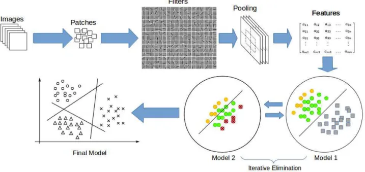
Figure 2. Overview of the proposed method. The data is pruned from spurious instances through eliminating the outliers. Then, the most confident in-class examples are utilized to build the models. These successive steps are repeated to construct the final model.

Figure 2 depicts the overview of FAME. Details will fol-low the review of the relevant studies and the benchmark datasets used in the experiments.

2. Related Works and Datasets

The work of Berg et al. is one of the first attempts in large scale face labeling through utilizing weakly-labeled web images [5, 4] with the “Labeled Faces in the Wild” (LFW) dataset introduced. Assuming that in an image at most one face corresponds to a name, they use names as constraints in clustering faces. With a similar constraint that faces in an image cannot be in the same cluster, Pham et al. [24] use a hierarchical agglomerative clustering method. With these methods it is likely to have clusters with several people mixed in, and multiple clusters for the same person, although ideally there should be a single cluster per person. [22] consider the problem as retrieving faces for a sin-gle query name, and then pruning the set from the irrelevant faces. With the assumption that the most similar subset of faces will correspond to the query, the densest component in the similarity graph is sought using a greedy method. For improvement, [13] uses a constraint for each image to con-tain a single instance of the queried person and assigns non-zero weights to nearest neighbors in the graph. They also handle multi-person naming and null assignments.

In [14] face-name association is tackled as a multiple in-stance learning problem over pairs of bags, where a pair of bags is labeled as positive if they share at least one name in their caption. Labeled Yahoo! News dataset is introduced

through manually annotating and extending LFW dataset. In [16], attribute and smile classifiers are proposed for verifying the identity of faces and Pub-Fig dataset, con-sisting of public figures on the web, is presented as having larger number of individuals and instances than LFW.

Recently, PubFig83, a subset of PubFig dataset with near-duplicates eliminated and individuals with large num-ber of instances selected, is provided for face identification task [25]. Inspired from biological systems, [25] consider V1-like features. In [8], person-specific subspace analysis is presented for identification of celebrities.

[20] defines the open-universe face identification prob-lem as identifying faces with one of the labeled categories in a dataset including distractor faces that do not belong to any of the labels. In this direction, [2] combines PubFig83, as being the set of labeled individuals, and LFW, as being the set of distractors.

Although search-based face annotation [31], which aims to annotate a face image through exploiting the labels of top ranked similar facial images, is similar to our problem in dealing with noisy labels, the problem different than ours where there is no query image to measure the similarity.

Inspired by the recently emerged studies on harvesting web for re-ranking of search results and building qualified training sets [11, 3, 17, 27, 7, 12] and on discovering dis-criminative patches [18, 29, 10, 15], we attack the prob-lem of face identification as the learning of models through pruning the weakly-labelled data.

3. Model Evolution

An important caveat in learning models from weakly-labeled data is the impurity of the collection. Spurious in-stances in the collection should be eliminated before gener-ating models for the categories. We present an approach for learning better models through iteratively pruning the data (see Figure 2). The proposed method allows the models to evolve through eliminating the outlier instances and sep-arating the most confident instances from the others with successive linear classifiers.

First, we learn a hyperplane that separates the initial set of candidate class instances from the large set of global negatives representing the rest of the world against the class of interest. Then, we select some fraction of the class in-stances distant from the separating hyperplane and use them as the category references as they are confidently classified against the rest of the world. We consider the rest of the class instances as possible spurious instances.

We then learn another model to capture in-class dissimi-larities between the category references and possible spuri-ous instances. We combine the confidence scores of the first and the second models as a measure of instance saliency. This combination allows us to benefit both from being dif-ferent from the rest of the world, and in-class affinity of the instance. We detect instances with the lowest confidence scores as the outliers for that iteration. These steps are it-erated multiple times up to a desired level of pruning (see Figure 3).

The large dimensional representation used (see Sec-tion 3.2) allows the diverse set of positive examples to be kept in the final model, but might cause computational bur-den with complicated learning models. Therefore, we lever-age simple linear regression (LR) models with L1 norm reg-ularization performing sparse feature selection as the learn-ing evolves.

Note that, our focus is to eliminate the outliers and purify the data while keeping most of the positives, and therefore it is not sufficient to only select most confident instances.

3.1. Iterative Data Elimination

Algorithm 1 summarizes our data elimination procedure. Here, C = {c1, c2, . . . cm} refers to the example face

im-ages collected for a class and N = {n1, n2, ..., nl} refers

to the vast numbers of global negatives. Each vector is a d dimensional representation of a single face image.

At each iteration t, the first LR model M1

learns a hyper-plane between the candidate class instances C and global negatives N . Then, C is divided into two subsets: p in-stances in C that are farthest from the hyperplane are kept as the candidate positive set (C+

) and the rest is considered as the negative set (C−_{) for the next model. C}+ _{is the set}

of salient instances representing the category references for the class and C−_{is the set of possible spurious instances.}

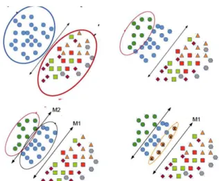
Figure 3. One step of model evolution. First, a model M1 is

learned to separate candidate category instances from global neg-atives. Then, the most confidently classified examples are

con-sidered as category references. Another model M2 is learned to

separate the category references from the other candidates. Spuri-ous instances that lie farthest from the hyperplane are eliminated.

Algorithm 1: FAME

1 C0←C

2 t ←1

3 while stoppingConditionN otSatisf ied() do

4 Mt1←LogisticRegression(Ct₋₁, N )

5 Ct+←selectT opP ositives(Ct₋₁, M

1 t, p) 6 C− t ←Ct₋₁−C + t 7 Mt2←LogisticRegresstion(C + t , Ct−) 8 [S− 1, S2−] ← getConf idenceScores(Ct−, M 1 tM 2 t) 9 Ot←selectOutliers(Ct−, S1−, S2−, o) 10 Ct←Ct −1−Ot 11 t ← t+ 1 12 end 13 C ← Ct 14 return C

The second LR model M2uses C+as positive and C−

as the negative set to learn the best possible hyperplane sep-arating them. For each instance in C−_{, by aggregating the}

confidence values of both models, o instances with the low-est scores are eliminated as the outliers.

This iterative procedure continues until it satisfies a stop-ping condition. We use M1

’s objective as the measure of data quality. As we incrementally remove poor instances, we expect to have better separation against the negative in-stances. If it saturates after a small number of iterations, we guarantee that at least 0.1 of the initial data is removed.

(a) (b) (c) (d)

Figure 4. Random set of filters learned from (a) whitened raw image pixels, (b) LBP encoded images. (c) Outliers for raw-image filters. (d) LBP encoding for an RGB image. We might observe eye or mount shaped filters from the raw image filters and more textural information from the LBP encoded filters. Outlier filters are very cluttered and observe low number of activations mostly from background patches.

3.2. Representation

Being effective, variants of Locally Binary Patterns (LBP) have been heavily utilized in the literature [1, 32, 6, 26]. Following the same direction we exploit LBP features. To represent face images we learn two distinct set of fil-ters by an unsupervised method as in [9] (Figure 4). First set is learned from the raw-pixel random patches extracted from grey-scale images. The second set is learned from LBP encoded images [1].

First set is receptive to edge- and corner-like structural points and the second set is sensitive to textural common-alities of the LBP histogram statistics. LBP encoded im-ages are invariant to illumination since the intensity rela-tions between pixels are considered instead of pixel values. We use rotation invariant LBP encoding [19] that gives bi-nary codes for each pixel. We convert these bibi-nary codes into corresponding integer values. A Gaussian filter is used to smooth out the heavy-tailed locations.

First, we extract a set of randomly sampled patches in the size of predefined receptive field. Then, contrast normal-ization is applied to each patch (for only raw-image filters) and patches are whitened to reduce the correlations among dimensions. These patches are clustered into K groups us-ing k-means. We perform thresholdus-ing to centroids with box-plot statistics over the activations counts to remove the outlier centroids. After the learning phase, centroid activa-tions are collected from receptive fields with small striding. We applied spatial average pooling onto five different grids (center and four quadrants). This yields a 5xK dimensional representation for each face, for each different set of filters. We use triangular activation function to map each receptive field to learned centroids. Assuming the patches assigned to outlier centroids are not relevant, we avoid them in pooling.

4. Experiments

For web-scale face verification, the task of given two face images deciding whether both belong to the same person, performances are closely approaching to human level [30]. We are interested in face identification, i.e. infer-ring the identity of people from their face images, and thus the setup is different than face verification.

4.1. Datasets

Training images are collected from Bing, and benchmark datasets FANlarge [21] and PubFig83 [25] are used to test.

Bing collection: For each name, 500 images are gath-ered using Bing image search1_{. Categories are chosen as}

the people having more than 50 annotated face images in FAN-large or PubFig83 datasets. In total, 22,6691 images are collected corresponding to 365 names in FAN-large, and 83 names in PubFig83. Additional 2,500 face images for queries “female face”, “male face”,‘ ‘face images” are collected to construct the global negatives. Face detector of [33] is used for detecting faces. Only the most confi-dent detection is selected from each image to be put into the initial pool of faces associated with the name. This pro-cess results in 450 faces on the average per category. Other detections are added to global negatives. Note that, this pro-cess assumes that the queried person appears as the largest and most visible face in the image, although this is not true in most of the cases and it may result in additional noise.

Test collections: EASY and ALL sets from FAN-large face dataset are used [21]. EASY subset includes faces larger than 60x70 pixels. ALL includes all faces with-out any size constraint. There are 138 names from EASY, and 365 from ALL subsets, with 23,952 and 199,295 im-ages respectively. On the average there are 541 imim-ages for each name. PubFig83 [25] dataset, the subset of well-known PugFig dataset with 83 different celebrities having at least 100 images, is also used in testing. In this set, near-duplicates and the ones that are no longer available at Inter-net are removed [2].

4.2. Implementation Details

The dataset is expanded with horizontally flipped images. Before learning filters from raw-pixel images, height of each grey-level face image is resized to 60 pixels and LBP images are resized to120 pixels. LBP encoding has been done by 16 different filter orientation and at radius 2. Random patches are sampled from images and contrast normalization is applied to only raw-pixel patches. Then, ZCA whitening transform is performed with ǫZCA= 0.5.

We use receptive field of 6x6 regions with 1 stride and learn 2,400 centroids for both raw-pixel and LBP encoded images. Hence, we come up with 2 (raw-pixel + LBP) x 5 (pooling grids) x 2,400 (centroids) dimensional feature rep-resentation of each image. We used Euclidean Distance. We detect the outliers by a threshold at the 99% upper whisker of the centroid activations. Our implementation of feature learning framework is aggregated upon the code by [9].

For iterative elimination, we train L1 norm Logistic Re-gression model with Gauss-Seidel algorithm [28] and final classification is done with Linear SVM through grafting al-gorithm [23] that learns sparse set of important features in-crementally by using gradient information. At each FAME iteration we eliminate five images. We stop when there is no improvement on the accuracy. If the classifier saturates so quickly, iteration continues until 10% of the instances are pruned. If we encounter memory constraints due to large number of global negatives, at each iteration we sample a different set of negative instances, to provide slightly differ-ent linear boundaries to detect differdiffer-ent spurious instances.

4.3. Evaluations

As seen in Figure 5, at each iteration of model evolution, dataset is divided into candidate positives (the most rep-resentative class instances), and possible negatives (where outliers are likely to be found). As Figure 6 shows, FAME is able to learn models from noisy datasets, while eliminat-ing the outliers at successive steps for a variety of people.

We evaluate the performance of FAME on PubFig83 dataset to test the effectiveness of some implementation de-tails. As Figure 7-(a) shows with the increasing number of iterations, more outliers are eliminated. Although some correct instances are also eliminated, the ratio is very low compared to the spurious instances. Moreover, observa-tions show that the eliminated positive examples are usually not in good quality and thus their elimination from the final model is not harmful but rather helpful as supported with the results in Figure 7-(b). As seen in Figure 7-(c) , we can achieve accuracies up to 75.2 on FAN-Large (EASY) and 79.8 on PubFig83 by removing one outlier at each iteration while we prefer to eliminate five outliers for the efficiency.

We also compared the performances obtained with dif-ferent features on PubFig83 dataset with the models learned from web. While LBP filters alone have the accuracy 60.7 and raw-pixel filters reach up to 71.6, the combination of both gives the highest performance of 79.3. As the results suggests, although LBP filters are not competitive with raw-pixel filters, its textural information is subsidiary to raw-pixel filters with increasing performance.

Figure 5. Some of the instances selected for confident positives

C+

, poor positives C−_{and outliers O for iterations t= 1 . . . 4.}

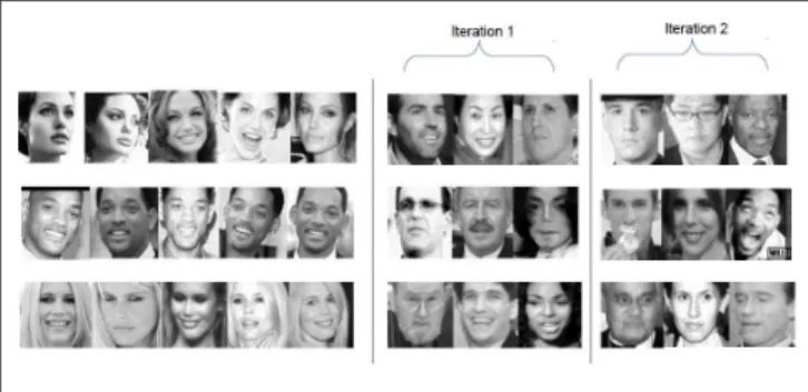
Figure 6. Final model faces and outliers in the first two iterations. Table 1. Accuracies on FAN-Large [21] EASY and ALL (FANL-E and FANL-A), and PubFig83 as well as on the held-out set of Bing collection. FAME-M1 uses only the model M1 that removes instances regarding global negatives. FAME-SVM uses SVM in training and FAME-LR is the proposed method using linear re-gression. Baseline method learns models directly from the original results without pruning. Comparisons are also given for [29].

- Bing FANL-E FANL-A PubFig83

Baseline 62.5 56.5 52.7 52.8 Singh et al. [29] 74.7 65.9 62.3 71.4 FAME-M1 78.6 68.3 60.2 71.7 FAME-SVM 81.4 73.1 65.4 76.8 FAME-LR 83.7 74.3 67.1 79.3

4.4. Comparisons

We compare FAME with the baseline method that learns models from the raw collection gathered through querying the name without any pruning. As seen in Table 1, with one versus all L1 norm Linear SVM model on the raw data, the performance is very low on all datasets.

We learn the models from web images and test them on the novel datasets (FAN-large and PubFig83) for the same categories. To test the effect of training and testing on the same type of dataset, we perform an experiment by dividing the collected Bing images into two subsets. As expected results are better on the same type of data, but FAME leads encouraging results even in the case of domain shift.

As the most similar data handling approach to ours, we compare FAME with the method of Singh et al. [29]

(Ta-2 4 6 8 10 12 0 5 10 15 20 25

#correct and #false outliers per FAME iteration

FAME iterations #instance #correct outliers #false outliers 2 4 6 8 10 12 0.65 0.7 0.75 0.8 0.85 0.9 0.95 1

X−val and Avg. M1 accuracy of selected classes per FAME iteration

FAME iterations accuracy(%) cross−val. accuracy Avg. M1 accuracy 1 2 3 4 5 6 7 8 9 10 64 66 68 70 72 74 76 78 80

# elimination per iter.

accuracy (%)

PubFig83 FAN−large (EASY)

(a) (b) (c)

Figure 7. (a) Correct versus false outlier detections until all the outliers are found for all classes. At each iteration values are aggregated with those of the previous one. (b) Cross-validation and M1 accuracies as the algorithm proceeds. There is a correlation between cross-validation and M1 models, without M1 models incurring over-fitting. (c) Number of outliers removed at each iteration versus accuracy. Elimination after some limit imposes degradation of final performance and eliminating one instance per iteration is the salient selection without any sanity check.

Table 2. Comparisons with other methods on PubFig83. [25] has single layer (S) and multi-layer (M) architectures. face.com API is also experienced in [25]. FAME is trained on PubFig83.

method [25]-S face.com [25] [2] [25]-M FAME

acc. 75.6 82.1 85.9 87.1 90.75

ble 1). [29] clusters the data to capture intra-cluster vari-ance and uncover the representative instvari-ances. They require to decide the optimal cluster number in advance and divide the problem into multiple homologous pieces to be solved separately, increasing the complexity of the proposed sys-tem. We solve intra-class modularity by using large di-mensional representations that supposedly make different classes linearly separable, even if classes include different modularities. We also find the representative instances by a supervised model which separates representative ones from the rest. Another difference lies in the philosophy. They aim to discover representative and discriminative set of in-stances whereas we aim to prune spurious ones. Hence, they need to keep all vast negative instances on memory but we can sample different subsets of global negatives and find corresponding outlier instances. It provides faster and easier way of data pruning. They divide each class into two sets and apply their scheme by interchanging data after each iteration like in the case of co-training learning procedure which demands large number of instances for reliable re-sults. We prefer to use all the class data at once in our par-ticular scheme. Comparisons with [29] show the superiority of FAME. We use the released code with up-limit settings of our resources.

To test the effectiveness of the proposed linear regression based model learning, we compare our results by using only the M1

model (FAME-M1) and using SVM for classifica-tion (FAME-SVM). As shown in Table 1, all FAME

mod-els outperform the baseline method as well as the method of [29] with a large improvement using the LR model.

Finally, we compare the performance of FAME on the PubFig83 dataset with the other state-of-the-art studies on face identification. In this case, unlike the previous exper-iments where we learned the models from web images, in order to make a fair comparison we learned the models from the same dataset. As seen in Table 2 FAME achieves the best accuracy in this setting. Referring back to Table 1, even with the domain adaptation setting where the model is learned from the noisy web images our results are com-parable to the most recent studies on face identification that train and test on the same dataset. Note that, the method of Pinto et al. [25] is similar to our classification pipeline but we prefer to learn the filters in an unsupervised way with the method of Coastes et al. [9]. In this setting, we also test the effect of number of centroids K. The accuracy for K=1500, 2000, 2400 are 84.90, 88.60, 90.75 respectively. Even for K=2000, FAME is better than the other methods.

5. Conclusions

We propose a novel method to prune the web images col-lected for a query to learn models to be used for classifica-tion on novel datasets. The proposed method outperforms the baseline and is comparable to state-of-the-art methods even within the difficulties of domain adaptation. In the fu-ture, we would like to test the method on the social network data with the faces of ordinary people.

Although the proposed method is tested for identification of faces, it is a general method that could be used for other domains as we aim to attack as our future work.

Acknowledgements

This study is partially supported by T ¨UB´ITAK project with grant number 112E174 and EU CHIST-ERA project MUCKE. This paper was also partially supported by the US Department of Defense, U. S. Army Research Office (W911NF-13-1-0277) and by the National Science Founda-tion under Grant No. IIS-1251187. The U.S. Government is authorized to reproduce and distribute reprints for Govern-mental purposes notwithstanding any copyright annotation thereon. Disclaimer: The views and conclusions contained herein are those of the authors and should not be interpreted as necessarily representing the official policies or endorse-ments, either expressed or implied, of ARO, the National Science Foundation or the U.S. Government.

References

[1] T. Ahonen, A. Hadid, and M. Pietikainen. Face description with local binary patterns: Application to face recognition. PAMI, 28(12), 2006.

[2] B. Becker and E. Ortiz. Evaluating open-universe face iden-tification on the web. In CVPR Workshop on Analysis and Modeling of Faces and Gestures, 2013.

[3] T. L. Berg and A. C. Berg. Finding iconic images. In CVPR Workshops, 2009.

[4] T. L. Berg, A. C. Berg, J. Edwards, and D. A. Forsyth. Who’s in the picture? In NIPS, 2004.

[5] T. L. Berg, A. C. Berg, J. Edwards, M. Maire, R. White, Y. W. Teh, E. Learned-Miller, and D. A. Forsyth. Names and faces in the news. In CVPR, 2004.

[6] D. Chen, X. Cao, F. Wen, and J. Sun. Blessing of dimension-ality: High-dimensional feature and its efficient compression for face verification. In CVPR, 2013.

[7] X. Chen, A. Shrivastava, and A. Gupta. Neil: Extracting visual knowledge from web data. In ICCV, 2013.

[8] G. Chiachia, N. Pinto, A. W. Rocha, W. Schultz, A. Falcao, and D. D. Cox. Person-specific subspace analysis for uncon-strained familiar face identification. In BMVC, 2012. [9] A. Coates, A. Y. Ng, and H. Lee. An analysis of

single-layer networks in unsupervised feature learning. In Inter-national Conference on Artificial Intelligence and Statistics, pages 215–223, 2011.

[10] C. Doersch, S. Singh, A. Gupta, J. Sivic, and A. A. Efros.

What makes paris look like paris? ACM Transactions on

Graphics (TOG), 31(4), 2012.

[11] R. Fergus, L. Fei-Fei, P. Perona, and A. Zisserman. Learn-ing object categories from google’s image search. In ICCV, 2005.

[12] E. Golge and P. Duygulu. Conceptmap:mining noisy web data for concept learning. In ECCV, 2014.

[13] M. Guillaumin, T. Mensink, J. Verbeek, and C. Schmid. Au-tomatic Face Naming with Caption-based Supervision. In CVPR, 2008.

[14] M. Guillaumin, J. Verbeek, and C. Schmid. Multiple instance metric learning from automatically labeled bags of faces. In ECCV, 2010.

[15] M. Juneja, A. Vedaldi, C. Jawahar, and A. Zisserman. Blocks

that shout: Distinctive parts for scene classification. In

CVPR, 2013.

[16] N. Kumar, A. C. Berg, P. N. Belhumeur, and S. K. Nayar. At-tribute and Simile Classifiers for Face Verification. In ICCV, 2009.

[17] L.-J. Li and L. Fei-Fei. Optimol: automatic online

pic-ture collection via incremental model learning. IJCV, 88(2), 2010.

[18] Q. Li, J. Wu, and Z. Tu. Harvesting mid-level visual concepts from large-scale internet images. CVPR, 2013.

[19] T. Ojala, M. Pietik¨ainen, and T. M¨aenp¨a¨a. Gray scale and rotation invariant texture classification with local binary pat-terns. In ECCV. 2000.

[20] E. G. Ortiz and B. C. Becker. Face recognition for web-scale datasets. CVIU, 118, 2014.

[21] M. ¨Ozcan, J. Luo, V. Ferrari, and B. Caputo. A large-scale

database of images and captions for automatic face naming. In BMVC, 2011.

[22] D. Ozkan and P. Duygulu. Interesting faces: A graph based approach for finding people in news. Pattern Recognition, 43(5), 2010.

[23] S. Perkins, K. Lacker, and J. Theiler. Grafting: Fast, in-cremental feature selection by gradient descent in function space. JMLR, 3, 2003.

[24] P. Pham, M. Moens, and T. Tuytelaars. Cross-media align-ment of names and faces. IEEE Transactions on Multimedia, 12(1):13–27, 2010.

[25] N. Pinto, Z. Stone, T. Zickler, and D. Cox. Scaling up

biologically-inspired computer vision: A case study in un-constrained face recognition on facebook. In CVPR Work-shops, 2011.

[26] S. Ren, X. Cao, Y. Wei, and J. Sun. Face alignment at 3000 fps by regressing local binary features. In CVPR, 2014. [27] F. Schroff, A. Criminisi, and A. Zisserman. Harvesting

im-age databases from the web. PAMI, 33(4), 2011.

[28] S. K. Shevade and S. S. Keerthi. A simple and efficient al-gorithm for gene selection using sparse logistic regression. Bioinformatics, 19(17), 2003.

[29] S. Singh, A. Gupta, and A. A. Efros. Unsupervised discovery of mid-level discriminative patches. In ECCV, 2012. [30] Y. Taigman, M. Yang, M. Ranzato, and L. Wolf. Deepface:

Closing the gap to human-level performance in face verifica-tion. In CVPR, 2014.

[31] D. Wang, S. C. Hoi, P. Wu, J. Zhu, Y. He, and C. Miao. Learning to name faces: A multimodal learning scheme for search-based face annotation. In SIGIR, 2013.

[32] L. Wolf, T. Hassner, and Y. Taigman. Descriptor based meth-ods in the wild. In ECCV Workshop on Faces in Real-Life Images, 2008.

[33] X. Zhu and D. Ramanan. Face detection, pose estimation, and landmark localization in the wild. In CVPR, 2012.