Chapter IV
Cross-Modal Correlation Mining
Using Graph Algorithms
Jia-Yu Pan
Carnegie Mellon University, USA Hyung-Jeong Yang
Chonnam National University, South Korea Christos Faloutsos
Carnegie Mellon University, USA Pinar Duygulu
Bilkent University, Turkey
Introduction
Advances in digital technologies make possible the generation and storage of large amount of
multimedia objects such as images and video clips. Multimedia content contains rich information in various modalities such as images, audios, video frames, time series, and so forth. However, making
AbstrAct
Multimedia objects like video clips or captioned images contain data of various modalities such as im-age, audio, and transcript text. Correlations across different modalities provide information about the multimedia content, and are useful in applications ranging from summarization to semantic captioning. We propose a graph-based method, MAGIC, which represents multimedia data as a graph and can find cross-modal correlations using “random walks with restarts.” MAGIC has several desirable properties: (a) it is general and domain-independent; (b) it can detect correlations across any two modalities; (c) it is insensitive to parameter settings; (d) it scales up well for large datasets; (e) it enables novel multimedia applications (e.g., group captioning); and (f) it creates opportunity for applying graph algorithms to multimedia problems. When applied to automatic image captioning, MAGIC finds correlations between text and image and achieves a relative improvement of 58% in captioning accuracy as compared to recent machine learning techniques.
rich multimedia content accessible and useful is not easy. Advanced tools that find characteristic patterns and correlations among multimedia content are required for the effective usage of multimedia databases.
We call a data object whose content is presented in more than one modality a mixed media object. For example, a video clip is a mixed media object with image frames, audios, and other informa-tion such as transcript text. Another example is a captioned image such as a news picture with an associated description, or a personal photograph annotated with a few keywords (Figure 1). In this chapter, we would use the terms medium (plural form media) and modality interchangeably.
It is common to see correlations among at-tributes of different modalities on a mixed media object. For instance, a news clip usually contains human speech accompanied with images of static scenes, while a commercial has more dynamic scenes with loud background music (Pan & Falout-sos, 2002). In image archives, caption keywords are chosen such that they describe objects in the
images. Similarly, in digital video libraries and entertainment industry, motion picture directors edit sound effects to match the scenes in video frames.
Cross-modal correlations provide helpful hints on exploiting information from different modalities for tasks such as segmentation (Hsu et al., 2004) and indexing (Chang, Manmatha, & Chua, 2005). Also, establishing associations between low-level features and attributes that have semantic meanings may shed light on multimedia understanding. For example, in a collection of captioned images, discovering the correlations between images and caption words could be use-ful for image annotation, content-based image retrieval, and multimedia understanding.
The question that we are interested in is “Given
a collection of mixed media objects, how do we find the correlations across data of various mo-dalities?” A desirable solution should be able to
include all kinds of data modalities, overcome noise in the data, and detect correlations between any subset of modalities available. Moreover, in
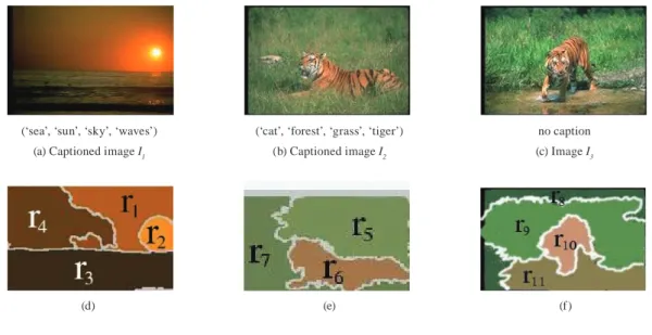
Figure 1. Three sample images: (a),(b) are captioned with terms describing the content; (c) is an image to be captioned. (d)(e)(f) show the regions of images (a)(b)(c), respectively.
(‘sea’, ‘sun’, ‘sky’, ‘waves’) (a) Captioned image I1
(‘cat’, ‘forest’, ‘grass’, ‘tiger’) (b) Captioned image I2
no caption (c) Image I3
terms of computation, we would like a method that scales well with respect to the database size and does not require human fine-tuning.
In particular, we want a method that can find correlations among all attributes, rather than just between specific attributes. For example, we want to find not just the image-term correlation between an image and caption terms, but also term-term and image-image correlations, using one single framework. This any-to-any medium correlation provides a greater picture of how attributes are correlated, for example, “which word is usually used for images with blue top,” “what words have related semantics,” and “what objects often appear together in an image.”
We propose a novel, domain-independent framework, MAGIC, for cross-modal correlation discovery. MAGIC turns the multimedia problem into a graph problem, by providing an intuitive framework to represent data of various modali-ties. The proposed graph framework enables the application of graph algorithms to multimedia problems.
In particular, MAGIC employs the random
walk with restarts technique on the graph to
discover cross-modal correlations.
In summary, MAGIC has the following ad-vantages:
• It provides a graph-based framework which is domain independent and applicable to mixed media objects which have attributes of various modalities.
• It can detect any-to-any medium correla-tions.
• It is completely automatic (its few parameters can be automatically preset).
• It can scale up for large collections of ob-jects.
In this study, we evaluate the proposed MAGIC method on the task of automatic image captioning. For automatic image captioning, the correlations
between image and text are used to predict caption words for an uncaptioned image.
Application 1 (automatic image captioning).
Given a set Icore of color images, each with caption words, find the best q (say, q=5) caption words for an uncaptioned image Inew.
The proposed method can also be easily ex-tended for various related applications such as captioning images in groups, or retrieving relevant video shots and transcript words.
In the following of this chapter, we will first discuss pervious attempts on multimedia cross-modal correlation discovery. Then, the proposed method, MAGIC, is introduced. We will show that MAGIC achieves a better performance than recent machine learning methods on automatic image captioning (a 58% improvement on cap-tioning accuracy). Several system issues are also discussed and we show that MAGIC is insensitive to parameter settings and is robust to variations in the graph.
relAted Work
Multimedia knowledge representation and ap-plication have attracted much research attention recently. Mixed media objects provide opportu-nities for finding correlations between low-level and concept-level features, and multimodal cor-relations have been shown useful for applications such as retrieval, segmentation, classification, and pattern discovery. In this section, we survey previous work on cross-modal correlation mod-eling. We also discuss previous work on image captioning, which is the application domain on which we evaluate our proposed model.
multimedia cross-modal correlation
Combining multimedia correlations in applica-tions leverages all available information and hasled to improved performances in segmentation (Hsu et al., 2004), classification (Lin & Haupt-mann, 2002; Vries, de Westerveld, & Ianeva, 2004), retrieval (Wang, Ma, Xue, & Li, 2004; Wu, Chang, Chang, & Smith, 2004; Zhang, Zhang, & Ohya, 2004), and topic detection (Duygulu, Pan, & Forsyth, 2004; Xie et al., 2005). One crucial step of fusing multimodal correlations into ap-plications is to detect and model the correlations among different data modalities.
We categorize previous methods for multi-media correlation modeling into two categories:
model-driven approaches and data-driven
ap-proaches. A model-driven method usually as-sumes a certain type of data correlations and focuses on fitting this particular correlation model to the given data. A data-driven method makes no assumption on the data correlations and finds correlations using solely the relationship (e.g., similarity) between data objects.
The model assumed by a model-driven method is usually hand-designed, based on the available knowledge to the domain. Model-driven methods provide a good way to incorporate prior knowledge into the correlation discovery process. However, the quality of the extracted correlations depends on the correctness of the assumed model. On the other hand, the performance of a data-driven method is less dependent on the available domain knowledge, but the ability to incorporating prior knowledge to guide the discovery process is more limited.
Previous model-driven methods have proposed a variety of models to extract correlations from multimodal data. Linear models (Srihari, Rao, Han, Munirathnam, & Xiaoyun, 2000; Li, Dimi-trova, Li, & Sethi, 2003) assume that data vari-ables have linear correlations. Linear models are computationally friendly, but may not approximate real data correlations well. More complex statisti-cal models have also been used: for example, the mixture of Gaussians (Vries, Westerveld, et al., 2004), the maximum-entropy model (Hsu et al., 2004), or the hidden Markov model (Xie, Kennedy
et al., 2005). Graphical models (Naphade, Kozint-sev, & Huang, 2001; Benitez & Chang, 2002; Jeon, Lavrenko, & Manmatha, 2003; Feng, Manmatha, & Lavrenko, 2004) have attracted much attention for its ability to incorporate domain knowledge into data modeling. However, the quality of the graphical model depends on the correctness of the embedded generative process, and sometimes the training of a complex graphical model can be computationally intractable.
Classifier-based models are suitable for fusing multimodal information when the application is data classification. Classifiers are useful in cap-turing discriminative patterns between different data modalities. To identify multimodal patterns for data classification, one can use either a multi-modal classifier which takes a multimulti-modal input, or a metaclassifier (Lin & Hauptmann, 2002; Wu et al., 2004) which takes as input the outputs of multiple unimodal classifiers.
Unlike a model-driven method that fits a pre-specified correlation model to the given dataset, a data-driven method finds cross-modal correlations solely based on the similarity relationship between data objects in the set. A natural way to present the similarity relationship between multimedia data objects is using a graph representation, where nodes symbolize objects, and edges (with weights) indicate the similarity between objects.
According to the application domains, different graph-based algorithms have been proposed to find data correlations from a graph representation of a dataset. For example, “spectral clustering” has been proposed for clustering data from different video sources (Zhang, Lin, Chang, & Smith, 2004), as well as for grouping relevant data of different modalities (Duygulu et al., 2004). Link analysis techniques have been used for deriving a multimodal (image and text) similarity function for Web image retrieval (Wang et al., 2004). For these methods, graph nodes are used to represent multimedia objects, and the focus is on finding cor-relations between data objects. This object-level
function between objects (for constructing graph edges) difficult, which is especially hard to obtain for complex multimedia objects.
In this chapter, we introduce MAGIC, a proposed data-driven method for finding cross-modal correlations in general multimedia settings. MAGIC uses a graph to represent the relations between objects and low-level attribute domains. By relating multimedia objects via the constituent single-modal domain tokens, MAGIC does not require object-level similarity functions, which are hard to obtain. Moreover, MAGIC does not need a training phase and is insensitive to parameter settings. Our experiments show that MAGIC can find correlations among all kinds of data modalities, and achieves good performance in real world multimedia applications such as image captioning.
Image captioning
Although a picture is worth a thousand words, extracting the abundant information from an image is not an easy task. Computational tech-niques are able to derive low-to-mid level features (e.g., texture and shape) from pixel information, however, the gap still exists between mid-level features and concepts used in human reasoning (Zhao & Grosky, 2001; Sebe, Lew, Zhou, Huang, & Bakker, 2003; Zhang, Zhang, et al., 2004). One consequence of this semantic gap in image retrieval is that the user’s need is not properly matched by the retrieved images, and may be part of the reason that practical image retrieval is yet to be popular.
Automatic image captioning, whose goal is to predict caption words to describe image content, is one research direction to bridge the gap between concepts and low-level features. Previous work on image captioning employs various approaches such as linear models (Mori, Takahashi, & Oka, 1999; Pan, Yang, Duygulu,
& Faloutsos, 2004), classifiers (Maron & Ratan, 1998), language models ( Duygulu, Barnard, de Freitas, & Forsyth, 2002; Jeon et al., 2003; Virga & Duygulu, 2005), graphical models (Barnard et al., 2003; Blei & Jordan, 2003), statistical models (Li & Wang, 2003; Feng et al., 2004; Jin, Chai, & Si, 2004). Interactive frameworks with user involvement have also been proposed (Wenyin et al., 2001).
Most previous approaches derive features from image regions (regular grids or blobs), and construct a model between images and words based on a reference captioned image set. Human annotators caption the reference images. However, we have no information about the association between individual regions and caption words. Some approaches attempt to explicitly infer the correlations between regions and words (Duygulu et al., 2002), with enhancements that take into consideration interactions between neighboring regions in an image (Li & Wang, 2003). Alter-natively, there are methods which model the col-lective correlations between regions and words of an image ( Pan, Yang, Faloutsos, & Duygulu, 2004a, 2004b).
Comparing the performance of different approaches is not easy. Although several bench-mark datasets are available, not every previous work reports results on the same subset of im-ages. Various metrics, such as accuracy, mean average precision, and term precision and recall, have been used by previous work to measure the performance. Since the perception of an image is subjective, some work also reports user evalu-ation of the captioning result. In this chapter, the proposed method is evaluated by its performance on image captioning, where the experiments are performed on the same dataset and evaluated using the same performance metric as previous work for fair comparison.
proposed grAph-bAsed
correlAtIon detectIon model
Our proposed method for mixed media correla-tion discovery, MAGIC, provides a graph-based representation for multimedia objects with data attributes of various modalities. A technique for finding any-to-any medium correlation, which is based on random walks on the graph, is also proposed. In this section, we explain how to gen-erate the graph representation and how to detect cross-modal correlations using the graph.graph representation for multimedia
In relational database management systems, a multimedia object is usually represented as a vector of m features/attributes (Faloutsos, 1996). The attributes must be atomic (i.e., taking single values) like “size” or “the amount of red color” of an image. However, for mixed media datasets, the attributes can be set-valued, such as the caption of an image (a set of words) or the set of regions of an image.Finding correlations among set-valued attri-butes is not easy. Elements in a set-valued attribute could be noisy or missing altogether, for example, regions may not be perfectly segmented from an image (noisy regions), and the image caption may be incomplete, leaving out some aspects of the content (noisy captions). Set-valued attributes of an object may have different numbers of elements, and the correspondence between set elements of different attributes is not known. For instance, a captioned image may have unequal numbers of caption words and regions, where a word may describe multiple regions and a region may be described by zero or more than one word. The detailed correspondence between regions and caption words is usually not given by human annotators.
We assume that the elements of a set-valued attribute are tokens drawn from a domain. We propose to gear our method toward set-valued
attributes, because they include atomic attributes as a special case and also smoothly handle the case of missing values (null set).
Definition 1 (domain and domain token). The
domain Di of (set-valued) attribute Ai is a collec-tion of atomic values, which we called domain tokens, which are the values that attribute Ai can take.
A domain can consist of categorical values, numerical values, or numerical vectors. For ex-ample, a captioned image has m = 2 attributes: The first attribute, “caption,” has a set of categorical values (English terms) as its domain; the second attribute, “regions,” is a set of image regions, each of which is represented by a p-dimensional vector of p features derived from the region (e.g., color histogram with p colors). As we will describe in the following experimental result section, we extract
p = 30 features from each region. To establish the
relation between domain tokens, we assume that we have a similarity function for each domain. Domain tokens are usually simpler than mixed media objects, and therefore, it is easier to define similarity functions on domain tokens than on mixed media objects. For example, for the attribute “caption,” the similarity function could be 1 if the two tokens are identical, and 0 if they are not. As for image regions, the similarity function could be the Euclidean distance between the p-dimensional feature vectors of two regions.
Assumption 1. For each domain Di (i=1, …, m), we are given a similarity function Simi(*,*) which assigns a score to a pair of domain tokens.
Perhaps surprisingly, with Definition 1 and As-sumption 1, we can encompass all the applications mentioned in the introduction. The main idea is to represent all objects and their attributes (domain tokens) as nodes of a graph. For multimedia objects with m attributes, we obtain a (m+1)-layer graph. There are m types of nodes (one for each attribute),
and one more type of nodes for the objects. We call this graph a MAGIC graph (Gmagic). We put an edge between every object-node and its cor-responding attribute-value nodes. We call these edges object-attribute-value links (OAV-links).
Furthermore, we consider that two objects are similar if they have similar attribute values. For example, two images are similar if they contain similar regions. To incorporate such information into the graph, our approach is to add edges to connect pairs of domain tokens (attribute values) that are similar, according to the given similar-ity function (Assumption 1). We call edges that connect nodes of similar domain tokens
nearest-neighbor links (NN-links).
We need to decide on a threshold for “close-ness” when adding NN-links. There are many ways to do this, but we decide to make the threshold adaptive: each domain token is connected to its k nearest neighbors. Computing nearest neighbors can be done efficiently, because we already have the similarity function Simi(*,*) for each domain Di
(Assumption 1). In the following section, we will discuss the choice of k, as well as the sensitivity of our results to k.
We illustrate the construction of the MAGIC graph by the following example.
Example 1. For the three images {I1, I2, I3} in
Figure 1, the corresponding MAGIC graph (Gmagic) is shown in Figure 2. The graph has three types of nodes: one for the image objects Ij’s (j=1,2,3); one for the regions rj’s (j=1,…,11), and one for the terms {t1,…,t8} = {sea, sun, sky, waves, cat, forest, grass, tiger}. Solid arcs are the object-at-tribute-value links (OAV-links). Dashed arcs are the nearest-neighbor links (NN-links), based on some assumed similarity function between re-gions. There is no NN-link between term-nodes, due to the definition of its similarity function: 1, if the two terms are the same; or 0 otherwise.
In Example 1, we consider only k = 1 nearest neighbor, to avoid cluttering the diagram. Because the nearest neighbor relationship is not symmetric and because we treat the NN-links as un-direc-tional, some nodes are attached to more than one link. For example, node r1 has two NN-links at-tached: r2’s nearest neighbor is r1, but r1’s nearest neighbor is r6. Figure 3 shows the algorithm for constructing a MAGIC graph.
We use image captioning only as an illustra-tion: the same graph framework can be generally used for other multimedia problems. For automatic image captioning, we also need to develop a method to find good caption words—words that correlate with an image, based on information in
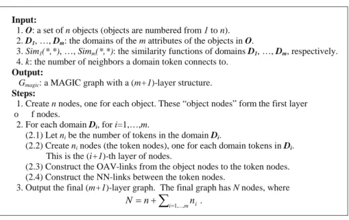
Figure 3. Algorithm for building the MAGIC graph: Gmagic = buildgraph(O, {D1,…, Dm}, {Sim1,…,Simm}, k)
Input:
1. O: a set ofn objects (objects are numbered from 1 to n).
2. D1, …, Dm: the domains of them attributes of the objects in O.
3. Sim1(*,*), …, Simm(*,*): the similarity functions of domains D1, …, Dm, respectively.
4. k: the number of neighbors a domain token connects to.
Output:
Gmagic: a MAGIC graph with a (m+1)-layer structure.
Steps:
1. Createn nodes, one for each object. These “object nodes” form the first layer
o f nodes.
2. For each domainDi, for i=1,…,m.
(2.1) Let ni be the number of tokens in the domainDi.
(2.2) Createni nodes (the token nodes), one for each domain tokens inDi.
This is the (i+1)-th layer of nodes.
(2.3) Construct the OAV-links from the object nodes to the token nodes. (2.4) Construct the NN-links between the token nodes.
3. Output the final (m+1)-layer graph. The final graph hasN nodes, where
= +
∑
=m i ni
n
N 1,..., .
Table 1. Summary of symbols used in the chapter
Symbol Description
N The number of objects in a mixed media dataset.
M The number of attributes (domains).
N The number of nodes in Gmagic.
E The number of edges in the graph Gmagic.
K Domain neighborhood size: the number of nearest neighbors that a domain token is connected to. C The restart probability of RWR (random walk with restarts, RWR).
Di The domain of the i-th attribute. Simi(*,*) The similarity function of the i-th domain.
Image captioning
Icore The given captioned image set (the core image set). Itest The set of to-be-captioned (test) images.
Inew An image in Itest.
Gcore The subgraph of Gmagic, which contains all images in Icore. Gaug The augmentation to Gcore, which contains information of image Itest.
GW The gateway nodes: the set of nodes of Gcore that are adjacent to Gaug.
Random walk with restarts (RWR) A The (column-normalized) adjacency matrix. The (i,j)-element of A is Ai,j.
vR The restart vector of the set of query objects R, where components correspond to query objects have value 1/|R|, while others have value 0).
uR The RWR scores of all nodes with respect to the set of query objects R. vq and uq The vR and uR for the singleton query set R={q}.
the Gmagic graph. For example, to caption the image
I3 in Figure 2, we need to estimate the correlation
degree of each term-nodes (t1, …, t8) to node I3, and the terms that are highly correlated with im-age I3 will be predicted as its caption words. The proposed method for finding correlated nodes in the Gmagic graph is described in the next section.
Table 1 summarizes the symbols we used in the chapter.
correlation detection with random
Walks
Our main contribution is to turn the cross-modal correlation discovery problem into a graph prob-lem. The previous section describes the first step of our proposed method: representing set-valued mixed media objects in a graph Gmagic. Given such a graph with mixed media information,
how do we detect the cross-modal correlations in the graph?
We define that a node A of Gmagic is correlated to another node B if A has an “affinity” for B. There are many approaches for ranking all nodes in a graph by their “affinity” for a reference node, for example, electricity-based approaches (Doyle & Snell, 1984; Palmer & Faloutsos, 2003), random walks (PageRank, topic-sensitive PageRank) (Brin & Page, 1998; Haveliwala, 2002; Haveli-wala, Kamvar, & Jeh., 2003), hubs and authorities
(Kleinberg, 1998), elastic springs (Lovász, 1996), and so on. Among them, we propose to use random
walk with restarts (RWR) for estimating the
af-finity of node B with respect to node A. However, the specific choice of method is orthogonal to our framework.
The “random walk with restarts” operates as follows: To compute the affinity uA(B) of node B for node A, consider a random walker that starts from node A. The random walker chooses randomly among the available edges every time, except that, before he makes a choice, he goes back to node A (restart) with probability c. Let uA(B) denote the steady state probability that our random walker will find himself at node B. Then, uA(B) is what we want, the affinity of B with respect to A. We also call uA(B) the RWR score of B with respect to A. The algorithm of computing RWR scores of all nodes with respect to a subset of nodes R is given in Figure 4.
Definition 2 (RWR score). The RWR score, uA(B),
of node B with respect to node A is the steady state probability of node B, when we do the random walk with restarts from A, as defined above.
Let A be the adjacency matrix of the given graph Gmagic, and let Ai,j be the (i,j)-element of A. In our experiments, Ai,j=1 if there is an edge between nodes i and j, and Ai,j=0 otherwise. To
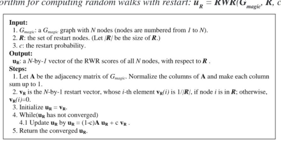
Figure 4. Algorithm for computing random walks with restart: uR = RWR(Gmagic, R, c) Input:
1. Gmagic: aGmagic graph with N nodes (nodes are numbered from 1 toN). 2. R: the set of restart nodes. (Let |R| be the size of R.)
3. c: the restart probability.
Output:
uR: aN-by-1 vector of the RWR scores of all N nodes, with respect to R . Steps:
1. LetA be the adjacency matrix of Gmagic. Normalize the columns ofA and make each column sum up to 1.
2. vR is the N-by-1 restart vector, whose i-th elementvR(i) is 1/|R|, if node i is in R; otherwise, vR(i)=0.
3. Initialize uR = vR.
4. While(uR has not converged)
4.1 Update uR by uR = (1-c)A uR + c vR .
perform RWR, columns of the matrix A are nor-malized such that elements of each column sum up to 1. Let uq be a vector of RWR scores of all
N nodes with respect to a restart node q, and vq
be the “restart vector,” which has all N elements zero, except for the entry that corresponds to node
q, which is set to 1. We can now formalize the
definition of the RWR score as follows:
Definition 3 (RWR score computation). The
N-by-1 steady state probability vector uq, which
contains the RWR scores of all nodes with respect to node q, satisfies the following equation: uq = (1-c)A uq + c vq,
where c is the restart probability of the RWR from node q.
The computation of RWR scores can be done efficiently by matrix multiplication (Step 4.1 in Figure 4). The computational cost scales linearly with the number of elements in the matrix A, that is , the number of graph edges determined by the given database. We keep track of the L1 distance between the current estimate of uq and the previ-ous estimate, and we consider the estimation of uq
converges when this L1 distance is less than 10-9. In
our experiments, the computation of RWR scores converges after a few (~10) iterations (Step 4 in Figure 4) and takes less than five seconds.
There-fore, the computation of RWR scales well with the database size. Moreover, MAGIC is modular and can continue improve its performance by including the best module (Kamvar, Haveliwala, Manning, & Golub, 2003; Kamvar, Haveliwala, & Golub, 2003) for fast RWR computation.
The RWR scores specify the correlations across different media and could be useful in many multimedia applications. For example, to predict the caption words for image I3 in Figure 1, we can compute the RWR scores uI3 of all nodes and report the top few (say, 5) term-nodes as caption words for image I3. Effectively, MAGIC exploits the correlations across images, regions and terms to caption a new image.
The RWR scores also enable MAGIC to detect any-to-any medium correlation. In our running example of image captioning, an image is captioned with the term nodes of highest RWR scores. In addition, since all nodes have their RWR scores, other nodes, say image nodes, can also be ranked and sorted, for finding images that are most related to image I3. Similarly, we can find the most relevant regions to image I3. In short, we can restart from any subset of nodes, say term nodes, and derive to-term, term-to-image, or term-to-any correlations. We will discuss more on this in the experimental result section. Figure 5 shows the overall procedure of using MAGIC for correlation detection.
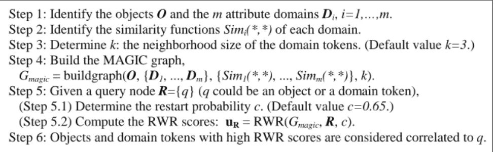
Figure 5. Steps for correlation discovery using MAGIC. Functions “buildgraph()” and “RWR()” are given in Figure 3 and Figure 4, respectively.
Step 1: Identify the objectsO and the m attribute domainsDi, i=1,…,m.
Step 2: Identify the similarity functions Simi(*,*) of each domain.
Step 3: Determine k: the neighborhood size of the domain tokens. (Default value k=3.) Step 4: Build the MAGIC graph,
Gmagic = buildgraph(O, {D1, ..., Dm}, {Sim1(*,*), ..., Simm(*,*)},k).
Step 5: Given a query node R={q} (q could be an object or a domain token), (Step 5.1) Determine the restart probabilityc. (Default valuec=0.65.)
(Step 5.2) Compute the RWR scores: uR = RWR(Gmagic, R, c).
ApplIcAtIon:
AutomAtIc ImAge cAptIonIng
Cross-modal correlations are useful for many mul-timedia applications. In this section, we present results of applying the proposed MAGIC method to automatic image captioning. Intuitively, the cross-modal correlations discovered by MAGIC are used in the way that an image is captioned automatically with words that correlate with the image content.We evaluate the quality of the cross-modal correlations identified by MAGIC in terms of captioning accuracy. We show experimental results to address the following questions: • Quality: Does MAGIC predict the correct
caption terms?
• Generality: Beside the image-to-term cor-relation for captioning, can MAGIC capture any-to-any medium correlation?
Our results show that MAGIC successfully exploits the image-to-term correlation to caption test images. Moreover, MAGIC is flexible and can caption multiple images as a group. We call this operation “group captioning” and present some qualitative results.
For detecting any-to-any medium correla-tions, we show that MAGIC can also capture same-modal correlations such as the term-term correlations: that is, “given a term such as ‘sky,’ find other terms that are likely to correspond to it.” Potentially, MAGIC is also capable of detecting other correlations such as the reverse captioning problem: that is, “given a term such as ‘sky,’ find the regions that are likely to correspond to it.” In general, MAGIC can capture any-to-any medium correlations.
dataset
Given a collection of captioned images Icore, how do we select caption words for an uncaptioned image Inew? For automatic image captioning, we
propose to caption Inew using the correlations between caption words and images in Icore.
In our experiments, we use the same 10 sets of images from Corel that are also used in previous work (Duygulu et al., 2002; Barnard et al. 2003), so that our results can be compared to the previous results. In the following, the 10 captioned image sets are referred to as the “001,” “002,” ..., “010” sets. Each of the 10 datasets has around 5,200 im-ages, and each image has about 4 caption words. These images are also called the core images from which we try to detect the correlations. For evaluation, each dataset is accompanied with a non-overlapping test set Itest of around 1,750 images for evaluating the captioning performance. Each test image has the ground truth caption.
Similar to previous work (Duygulu et al,. 2002; Barnard et al., 2003), each image is represented by a set of image regions. Image regions are extracted using a standard segmentation tool (Shi & Malik, 2000), and each region is represented as a 30-di-mensional feature vector. The regional features include the mean and standard deviation of RGB values, average responses to various texture filters, its position in the entire image layout, and some shape descriptors (e.g., major orientation and the area ratio of bounding region to the real region). Together, regions extracted from an image form a set-valued attribute “regions” of the object “im-age.” In our experiments, an image has 10 regions on average. Some examples of image regions are shown in Figure 1 (d), (e), and (f).
The exact region segmentation and feature extraction details are orthogonal to our ap-proach—any published segmentation methods and feature extraction functions (Faloutsos, 1996) will suffice. All our MAGIC method needs is a
black box that will map each color image into a set of zero or more feature vectors.
We want to stress that there is no given in-formation about which region is associated with which term—all we know is that a set of regions co-occurs with a set of terms in an image. That is, no alignment information between individual regions and terms is available.
Therefore, a captioned image becomes an object with two set-valued attributes: “regions” and “terms.” Since the regions and terms of an image are correlated, we propose to use MAGIC to detect this correlation and use it to predict the missing caption terms correlated with the uncap-tioned test images.
constructing the mAgIc graph
The first step of MAGIC is to construct the MAGIC graph. Following the instructions for graph con-struction in Figure 3, the graph for captioned images with attributes “regions” and “terms” will be a 3-layer graph with nodes for images, regions and terms. To form the NN-links, we define the distance function (Assumption 1) between two regions (tokens) as the L2 norm between their feature vectors. Also, we define that two terms are similar if and only if they are identical, that is, no term is any other’s neighbor. As a result, there is no NN-link between term nodes.
For results shown in this section, the number of nearest neighbors between attribute (domain) tokens is k=3. However, as we will show later in the experimental result section, the captioning accuracy is insensitive to the choice of k. In total, each dataset has about 50,000 different region tokens and 160 words, resulting in a graph Gmagic with about 55,500 nodes and 180,000 edges. The graph based on the core image set Icore captures the correlations between regions and terms. We call such graph the “core” graph.
How do we caption a new image, using the information in a MAGIC graph? Similar to the
core images, an uncaptioned image Inew is also an
object with set-valued attributes: “regions” and “caption,” where attribute “caption” has null value. To find caption words correlated with image Inew, we propose to look at regions in the core image set that are similar to the regions of Inew, and find the words that are correlated with these core im-age regions. Therefore, our algorithm has two main steps: finding similar regions in the core image set (augmentation) and identifying cap-tion words (RWR). Next, we define “core graph,” “augmentation” and “gateway nodes,” to facilitate the description of our algorithm.
Definition 4 (core graph, augmentation, and gateway nodes). For automatic image
caption-ing, we define the core of the graph Gmagic, Gcore,
be the subgraph that constitutes information of the given captioned images Icore. The graph Gmagic for captioning a test image Inew is an augmented graph, which is the core Gcore augmented with the region-nodes and image-node of Inew. The augmentation subgraph is denoted as Gaug, and hence the overall Gmagic=Gcore∪Gaug. The nodes of the core subgraph Gcore that are adjacent to the augmentation Gaug are called the gateway nodes, GW.
As an illustration, Figure 2 shows the graph
Gmagic for two core (captioned) images Icore={I1, I2} and one test (to-be-captioned) image Itest={I3},
with the parameter for NN-links k=1. The core subgraph Gcore contains region nodes {r1, ..., r7}, image nodes {I1, I2}, and all the term nodes {t1, ...,
t8}. The augmentation Gaug contains region nodes
{r8, ..., r11} and the image node {I3} of the test image. The gateway nodes GW = {r5, r6, r7} that bridge subgraphs Gcore and Gaug are the nearest neighbors of the test image’s regions {r8, ..., r11}.
In our experiments, the gateway nodes are always region-nodes in Gcore that are the nearest neighbors of test image’s regions. Different test images have different augmented graphs and gate-way nodes. However, since we will caption only one test image at a time, we will use the symbols
Gaug and GW to represent the augmented graph and
gateway nodes of the test image in question. To sum up, for image captioning, the proposed method first constructs the core graph Gcore, ac-cording to the given set of captioned images Icore. Then, each test image Inew is captioned one by one, in two steps: augmentation and RWR. In the augmentation step, the Gaug subgraph of the test image Inew is connected to Gcore via the gateway nodes - the k nearest neighbors of each region of
Inew. In the RWR step, we do RWR on the whole
augmented graph Gmagic=Gcore∪Gaug, restarting
from the test image-node, to identify the cor-related words (term-nodes). The g term-nodes with highest RWR scores will be the predicted caption for image Inew. Figure 6 gives the details of our algorithm for image captioning.
captioning Accuracy
We measure captioning performance by the captioning accuracy. The captioning accuracy is defined as the fraction of terms correctly pre-dicted. Following the same evaluation procedure as that in previous work (Duygulu et al., 2002; Barnard et al., 2003), for a test image which has
g ground-truth caption terms, MAGIC will also
predict g terms. If p of the predicted terms are correct, then the captioning accuracy acc on this test image is defined as:
acc = p/g.
The average captioning accuracy accmean on a set of T test images is defined as:
1 1 T mean i i acc acc T = =
∑
,where acci is the captioning accuracy on the i-th test image.
Figure 7 shows the average captioning ac-curacy on the 10 image sets. We compare our results with the method in (Duygulu et al., 2002), which considers the image captioning problem as a statistical translation modeling problem and solves it using expectation-maximization (EM). We refer to their method as the “EM” approach. The x-axis groups the performance numbers of MAGIC (white bars) and EM (black bars) on the 10 datasets. On average, MAGIC achieves cap-tioning accuracy improvement of 12.9 percentage points over the EM approach, which corresponds to a relative improvement of 58%.
The EM method assumes a generative model of caption words given an image region. The model assumes that each region in an image is considered separately when the caption words for an image are “generated.” In other words, the model does not take into account the potential correlations among the “same-image regions”—regions from a same image. On the other hand, MAGIC incorporates such correlations, by connecting nodes of the “same-image regions” to the same image node in the MAGIC graph. Ignoring the correlations between “same-image regions” could
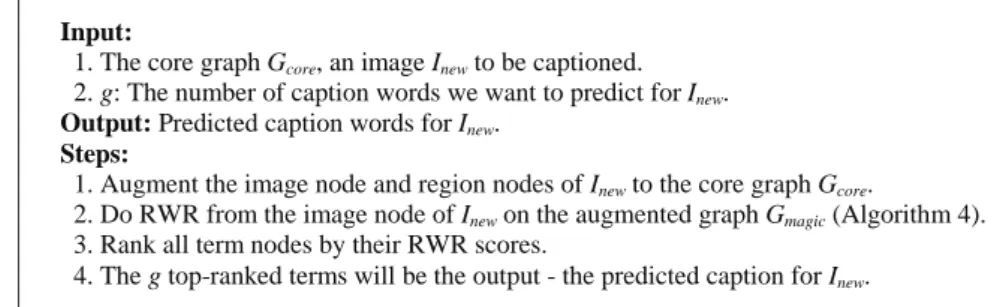
Figure 6. The proposed steps for image captioning, using the MAGIC framework
Input:
1. The core graphGcore, an imageInew to be captioned.
2. g: The number of caption words we want to predict forInew.
Output: Predicted caption words forInew.
Steps:
1. Augment the image node and region nodes ofInew to the core graph Gcore.
2. Do RWR from the image node ofInew on the augmented graph Gmagic (Algorithm 4).
3. Rank all term nodes by their RWR scores.
Figure 7. Comparing MAGIC to the EM method. The parameters for MAGIC are c=0.66 and k=3. The x-axis shows the 10 datasets, and the y-axis is the average captioning accuracy over all test images in a set.
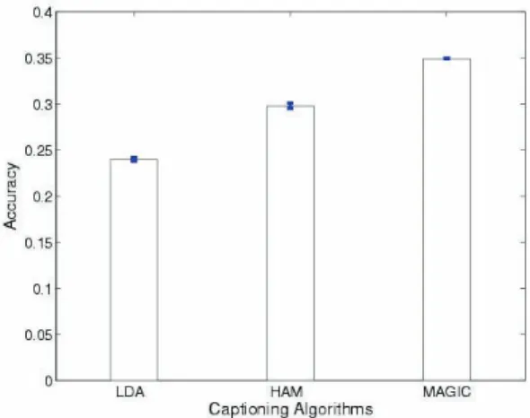
Figure 8. Comparing MAGIC with LDA and HAM. The mean and variance of the average accuracy over the 10 Corel datasets are shown at the y-axis - LDA: (μ, σ2)=(0.24,0.002); HAM: (μ, σ2)=(0.298,0.003); MAGIC: (μ, σ2)=(0.3503,
0.0002). μ: mean average accuracy. σ2: variance
of average accuracy. The range of the error bars at the top of each bar is 2σ.
be a reason why the EM method performs not as good as MAGIC.
We also compare the captioning accuracy with even more recent machine vision methods: the hierarchical aspect models method (“HAM”) and the latent dirichlet allocation model (“LDA”) (Barnard et al., 2003). The methods HAM and LDA are applied to the same 10 Corel datasets, and the average captioning accuracy (averages over the test images) from each set is computed. We summarize the overall performances of a method by taking the mean and variance of the 10 average captioning accuracy values on the 10 datasets. Figure 8 compares MAGIC with LDA and HAM, in terms of the mean and variance of the average captioning accuracy over the 10 datasets. Although both HAM and LDA improve on the EM method, they both lose to our generic MAGIC approach (35%, vs. 29% and 25%). It is also interesting that MAGIC gives significantly lower variance, by roughly an order of magnitude: 0.002 vs. 0.02 and 0.03. A lower variance indicates
that the proposed MAGIC method is more robust to variations among different datasets.
The EM, HAM, and LDA methods all assume a generative model on the relationship among image regions and caption words. For these models, the quality of the data correlations depends on how good the assumed model matches the real data characteristics. Lacking correct insights to the behavior of a dataset when designing the model may hurt the performance of these methods.
Unlike EM, HAM, and LDA, which are meth-ods specifically designed for image captioning, MAGIC is a method for general correlation detec-tion. We are pleasantly surprised that a generic method like MAGIC could outperform those domain-specific methods.
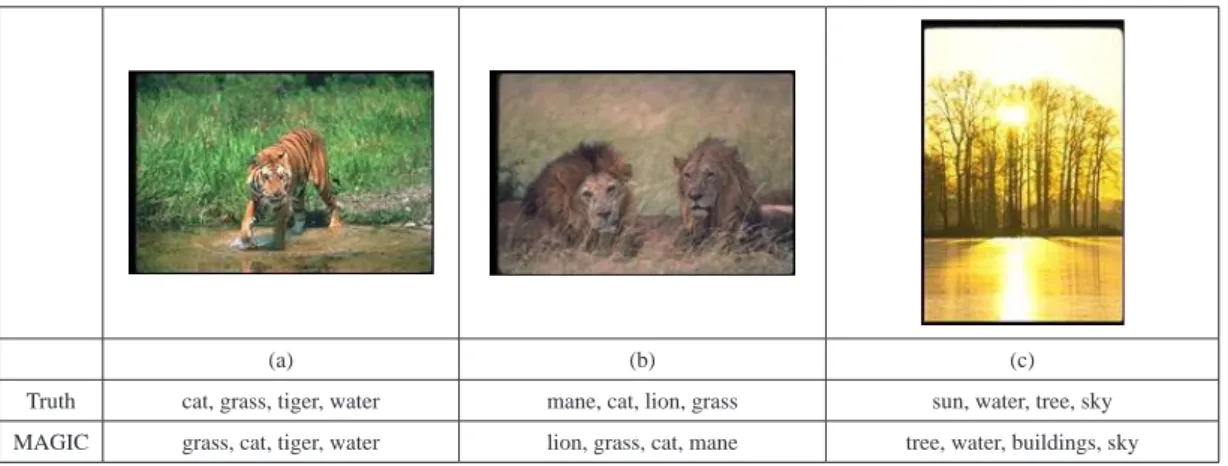
Figure 9 shows some examples of the cap-tions given by MAGIC. For the test image I3 in Figure 1, MAGIC captions it correctly (Figure 9a). In Figure 9b, MAGIC surprisingly gets the seldom-used word “mane” correctly; however, it
mixes up “buildings” with “tree” for the image in Figure 9c.
generalization
MAGIC treats information from all media uni-formly as nodes in a graph. Since all nodes are basically the same, we can do RWR and restart from any subset of nodes of any medium, to detect any-to-any medium correlations. The flexibility of our graph-based framework also enables novel applications, such as captioning images in groups (group captioning). In this subsection, we show results on (a) detecting the term-to-term correla-tion in image capcorrela-tioning datasets, and (b) group captioning.
Our image captioning experiments show that MAGIC successfully exploits the image-to-term correlation in the MAGIC graph (Gmagic) for image captioning. However, the MAGIC graph Gmagic contains correlations among all media (image, region, and term), not just between images and terms. To show how well MAGIC works on discovering correlations among all media, we design an experiment to extract the term-to-term correlation in the graph Gmagic and identify cor-related captioning terms.
We use the same 3-layer MAGIC core graph
Gcore constructed in the previous subsection for
automatic image captioning (Figure 2). Given a query term t, we use RWR to find other terms correlated with it. Specifically, we perform RWR, restarting from the query term(-node). The terms whose corresponding term-nodes receive high RWR scores are considered correlated with the query term.
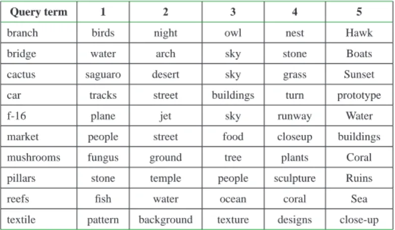
Table 2 shows the top 5 terms with the highest RWR scores for some query terms. In the table, each row shows a query term at the first column, followed by the top 5 correlated terms selected by MAGIC (sorted by their RWR scores). The selected terms have meanings that are semanti-cally related with the query term. For example, the term “branch,” when used in image captions, is strongly related to forest- or bird- related concepts. MAGIC shows exactly this, correlating “branch” with terms such as “birds,” “owl,” and “nest.”
Another subtle observation is that our method does not seem to be biased by frequently appeared words. In our collection, the terms “water” and “sky” appear more frequently in image captions, that is, they are like terms “the” and “a” in nor-mal English text. Yet, these frequent terms do
not show up too often in Table 2, as a correlated
term of a query term. It is surprising, given that
Figure 9. Image captioning examples: For MAGIC, terms with highest RWR scores are listed first
(a) (b) (c)
Truth cat, grass, tiger, water mane, cat, lion, grass sun, water, tree, sky
we do nothing special when using MAGIC: no tf/idf weighting, no normalization, and no other domain-specific analysis. We just treat these frequent terms as nodes in our MAGIC graph, like any other nodes.
Another advantage of the proposed MAGIC method is that it can be easily extended to caption a group of images, considering the whole group at once. This flexibility is due to the graph-based framework of MAGIC, which allows augmenta-tion of multiple nodes and doing RWR from any subset of nodes. To the best of our knowledge, MAGIC is the first method that is capable of do-ing group captiondo-ing.
Application 2 (group captioning). Given a set
Icore of captioned images and a (query) group of uncaptioned images {I’1, ..., I’t}, find the best g (say, g=5) caption words to assign to the group.
Possible applications for group captioning include video segment captioning, where a video segment is captioned according to the group of keyframes associated with the segment. Since keyframes in a video segment are usually related, captioning them as a whole can take into account the inter-keyframe correlations, which are missed if each keyframe is captioned separately.
Accu-rate captions for video segments may improve performances on tasks such as video retrieval and classification.
The steps to caption a group of images are similar to those for the single-image captioning outlined in Figure 6. A core MAGIC graph is still used to capture the mixed media information of a given collection of captioned images. The dif-ferent steps for doing group captioning are: First, instead of augmenting the single query image to the core and restarting from it, we augment all t images in the query group {I’1, ..., I’t} to the core. Then, the RWR step is performed by randomly restarts from one of the images in the group (i.e., each of the t query image has probability 1/t to be the restart node).
Figure 10 shows the result of using MAGIC for captioning a group of three images. MAGIC finds reasonable terms for the entire group of im-ages: “sky,” “water,” “tree,” and “sun.” Captioning multiple images as a group takes into consideration the correlations between different images in the group, and in this example, this helps reduce the scores of irrelevant terms such as “people.” In contrast, when we caption these images individu-ally, MAGIC selects “people” as caption words for images in Figure 10(a) and (b), which do not contain people-related objects.
Table 2. Correlated terms of some query terms
Query term 1 2 3 4 5
branch birds night owl nest Hawk
bridge water arch sky stone Boats
cactus saguaro desert sky grass Sunset
car tracks street buildings turn prototype
f-16 plane jet sky runway Water
market people street food closeup buildings
mushrooms fungus ground tree plants Coral
pillars stone temple people sculpture Ruins
reefs fish water ocean coral Sea
system Issues
MAGIC provides an intuitive framework for detecting cross-modal correlations. The RWR computation in MAGIC is fast and it scales linearly with the graph size. For example, a straightforward implementation of RWR can caption an image in less than five seconds.
In this section, we discuss system issues such as parameter configuration and fast computation. In particular, we present results showing: • MAGIC is insensitive to parameter
set-tings.
• MAGIC is modular that we can easily employ the best module to date to speedup MAGIC.
optimization of parameters
There are several design decisions to be made when employing MAGIC for correlation detection:
what should be the values for the two parameters: the number of neighbors k of a domain token, and the restart probability c of RWR? And, should we assign weights to edges, according to the types of their end points? In this section, we empirically
show that the performance of MAGIC is
insensi-tive to these settings, and provide suggestions on determining reasonable default values.
We use automatic image captioning as the ap-plication to measure the effect of these parameters. The experiments in this section are performed on the same 10 captioned image sets (“001”, ..., “010”) described in previous sections, and we measure how the values of the parameters, such as k, c, and the weights of the links of the MAGIC graphs, effect the captioning accuracy.
Number of Neighbors k. The parameter k speci-fies the number of nearest domain tokens to which a domain token connects via the NN-links. With these NN-links, objects having little difference in their attribute values will be closer to each other in the graph, and therefore, are considered more correlated by MAGIC. For k = 0, all domain tokens are considered distinct; for larger k, our application is more tolerant to the difference in attribute values.
We examine the effect of various k values on image captioning accuracy. Figure 11 shows the captioning accuracy on the dataset “006,” with the restart probability c = 0.66. The captioning accuracy increases as k increases from k = 1, and reaches a plateau between k = 3 and 10. The
Figure 10. Group captioning by MAGIC: Caption terms with highest RWR scores are listed first
(a) (b) (c)
Truth sun, water, tree, sky sun, clouds, sky, horizon sun, water
plateau indicates that MAGIC is insensitive to the value of k. Results on other datasets are similar, showing a plateau between k = 3 and 10.
In hindsight, with only k = 1, the collection of regions (domain tokens) is barely connected, missing important connections and thus leading to poor performance on detecting correlations. At the other extreme, with a high value of k, ev-erybody is directly connected to evev-erybody else and there is no clear distinction between really close neighbors or just neighbors. For a medium value of k, the NN-links apparently capture the correlations between the close neighbors and avoid noise from remote neighbors. Small deviations from that value make little difference, which is probably because that the extra neighbors we add (when k increases), or those we retained (when
k decreases), are at least as good as the previous
ones.
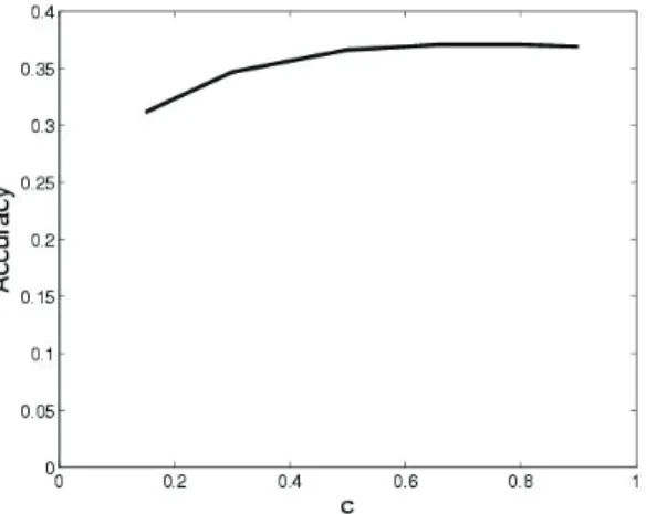
Restart Probability c. The restart probability
c specifies the probability to jump back to the
restarting node(s) of the random walk. Higher value of c implies giving higher RWR scores to nodes closer in the neighborhood of the restart node(s). Figure 12 shows the image captioning accuracy of MAGIC with different values of c. The dataset is “006,” with the parameter k = 3. The accuracy reaches a plateau between c = 0.5 and 0.9, showing that the proposed MAGIC method is insensitive to the value of c. Results on other datasets are similar, showing a plateau between
c = 0.5 and 0.9.
For Web graphs, the recommended value for
c is typically c = 0.15 (Haveliwala et al., 2003).
Surprisingly, our experiments show that this choice does not give good performance. Instead, good quality is achieved for c = 0.6~0.9. Why is this discrepancy?
We conjecture that what determines a good value for the restart probability is the diameter of the graph. Ideally, we want our random walker to have a nontrivial chance to reach the outskirts
Figure 11. The plateau in the plot shows that the captioning accuracy is insensitive to value of the number of nearest neighbors k. Y-axis: Average accuracy over all test images of dataset “006”. The restart probability is c=0.66.
Figure 12. The plateau in the plot shows that the captioning accuracy is insensitive to value of the restart probability c. Y-axis: Average accuracy over all images of dataset “006.” The number of nearest neighbors per domain token (region) is k = 3.
of the whole graph. If the diameter of the graph is d, the probability that the random walker (with restarts) will reach a point on the periphery is proportional to (1-c)d, that is , the probability of not restarting for d consecutive moves.
For the Web graph, the diameter is estimated to be d = 19 (Albert, Jeong, & Barabasi, 1999). This implies that the probability pperiphery for the random walker to reach a node in the periphery of the Web graph is roughly:
pperiphery = (1-c)19 = (1-0.15)19 = 0.045 .
In our image captioning experiments, we use graphs that have three layers of nodes (Figure 2). The diameter of such graphs is roughly d = 3. If we demand the same pperiphery = 0.045, then the c value for our 3-layer graph would be:
(1-0.15)19 = (1-c)3, ⇒c = 0.65,
which is much closer to our empirical observa-tions. Of course, the problem requires more careful analysis—but we are the first to show that c = 0.15 is not always optimal for random walk with restarts.
Link weights. MAGIC uses a graph to encode the relationship between mixed media objects and their attributes of different media. The OAV-links in the graph connect objects to their domain tokens (Figure 2). To give more attention to an attribute domain D, we can increase the weights of OAV-links that connect to the tokens of domain D. Should we treat all media equally,
or should we weight OAV-links according to their associated domains? How should we weight the OAV-links? Could we achieve better performance on weighted graphs?
We investigate how the change on link weights influences the image captioning accuracy. Table
3 shows the captioning accuracy on dataset “006” when different weights are assigned on the OAV-links to regions (weight wregion) and those to terms (wterm). Specifically, the elements Ai,j of the adjacency matrix A will now take values wregion or wterm, besides values 0 and 1, depending on the type of link Ai,j corresponds to. For all cases, the number of nearest neighbors is k = 3 and the restart probability is c = 0.66. The case where (wregion, wterm) = (1,1) is that of the unweighted graph, and is the result we reported in Figure 7. As link weights vary from 0.1, 1 to 10, the captioning accuracy is basically unaffected. The results on other datasets are similar—captioning accuracy is at the same level on a weighted graph as on the unweighted graph.
This experiment shows that an unweighted graph is appropriate for our image captioning application. We speculate that an appropriate weighting for an application depends on proper-ties such as the number of attribute domains (i.e., the number of layers in the graph), the average size of a set-valued attribute of an object (such as, average number of regions per image), and so on. We plan to investigate more on this issue in our future work.
speedup graph construction by
Approximation
The proposed MAGIC method encodes a mixed media dataset as a graph, and employs the RWR algorithm to find cross-modal correlations. The construction of the Gmagic graph is intuitive and straightforward, and the RWR computation is light and linear to the database size. One step that is relatively expensive is the construction of NN-links in a MAGIC graph.
When constructing the NN-links of a MAGIC graph, we need to compute the nearest neighbors for every domain token. For example, in our image captioning experiments, to construct the NN-links among region-nodes, k-NN searches
are performed about 50,000 times (one for each region token) in the 30-dimensional region-fea-ture space.
In MAGIC, the NN-links are proposed to capture the similarity relation among domain tokens. The goal is to associate similar tokens to each other, and therefore, it could be suffice to have the NN-links connect to neighbors that are close enough, even if they are not exactly the closest ones. The approximate nearest neighbor search is usually faster, by trading accuracy for speed. The interesting questions are: How much
speedup could we gain by allowing approximate NN-links? How much is the performance reduc-tion by approximareduc-tion?
For efficient nearest neighbor search, one common way is to use a spatial index, such as R+-tree (Sellis, Roussopoulos, & Faloutsos, 1987),
to find exact nearest neighbors in logarithmic time. Fortunately, MAGIC is modular and we can pick the best module to perform each step. In our experiments, we use the approximate nearest neighbor searching (ANN) (Arya, Mount, Netan-yahu, Silverman, & Wu, 1998), which supports both exact and approximate nearest neighbor search. ANN estimates the distance to a nearest neighbor up to (1+ε) times of the actual distance:
ε=0 means exact search with no approximation;
bigger ε values give rougher estimation.
Table 4 lists the average wall clock time to compute the top 10 neighbors of a region in the 10 Corel image sets of our image captioning experiments. The table shows the efficiency/ac-curacy trade off on constructing the NN-links among image regions. In an approximate nearest neighbor search, the distance to a neighboring
Table 3. Captioning accuracy is insensitive to various weight settings on OAV-links to the two media: region (weight wregion) and term (wterm).
wregion
wterm 0.1 1 10
0.1 0.370332 0.371963 0.370812
1 0.369900 0.370524 0.371963
10 0.368969 0.369181 0.369948
Table 4. The efficiency/accuracy trade off of constructing NN-links using an approximate method (ANN). ε=0 indicates the exact nearest neighbor computation. Elapse time: average wall clock time for one nearest neighbor search. Speedup: the ratio of the time of sequential search (SS) and that of an ANN search. The error is measured as the percentage of mistakes made by approximation on the k nearest neighbors. The symbol “-” means zero error.
Approximate Nearest Neighbor Search Sequential search
(SS)
ε=0 ε=0.2 ε=0.8
Elapse time (msec.) 3.8 2.4 0.9 46
Speedup to SS 12.1 19.2 51.1 1
Error (in top k=10) - 0.0015% 1.67%
-region is approximated to within (1+ε) times of the actual distance. The speedup of using the approximate method is compared to the sequen-tial search method (SS). In our experiments, the sequential search method is implemented in C++ and compiled with the code optimization, using the command “g++ -O3.”
Compared to the sequential search, the speedup of using the ANN method increases from 12.1 to 51.1, from the exact search (ε=0) to a rough ap-proximation of (ε=0.8). For the top k = 3 nearest neighbors (the setting used in most of our experi-ments), the error percentage is at most 0.46% for the roughest approximation, which is equivalent to making one error in every 217 NN-links.
We conduct experiments to investigate the effect on captioning accuracy from using the approximate NN-links. In general, the small differences on NN-links due to approximation do not change the characteristic of the MAGIC graph significantly, and has limited affect on the performance of image captioning (Figure 13). At the approximation level ε = 0.2, we achieve a speedup of 19.1 times and surprisingly that no error is made on the NN-links in the MAGIC graph, and therefore the captioning accuracy is the same as exact computation. At the approximation level ε
= 0.8, which gives an even better speedup of 51.1
times, the average captioning accuracy decreases by just 1.59 percentage point (averaged over the 10 Corel image sets). Therefore, by using an ap-proximate method, we can significantly reduce the time to construct the MAGIC graph (up to 51.1 times speedup), with almost no decrease on the captioning accuracy.
conclusIon
Mixed media objects such as captioned images or video clips contain attributes of different modali-ties (image, text, or audio). Correlations across different modalities provide information about the multimedia content, and are useful in
appli-cations ranging from summarization to semantic captioning. In this chapter, we develop MAGIC, a graph-based method for detecting cross-modal correlations in mixed media dataset.
There are two challenges in detecting cross-modal correlations, namely, representation of attributes of various modalities and the detection of correlations among any subset of modalities. MAGIC turns the multimedia problem into a graph problem, and provides an intuitive solution that easily incorporates various modalities. The graph framework of MAGIC creates opportunity for ap-plying graph algorithms to multimedia problems. In particular, MAGIC finds cross-modal correla-tions using the technique of random walk with restarts (RWR), which accommodates set-valued attributes and noise in data with no extra effort.
We apply MAGIC for automatic image caption-ing. By finding robust correlations between text and image, MAGIC achieves a relative improve-ment by 58% in captioning accuracy as compared
Figure 13. Speeding up NN-links construction by ANN (with ε=0.8) reduces captioning accuracy by just 1.59% on the average. X-axis: 10 datasets. Y-axis: average captioning accuracy over test im-ages in a set. In this experiment, the parameters are c=0.66 and k=3.
to recent machine learning techniques (Figure 8). Moreover, the MAGIC framework enables novel data mining applications, such as group
captioning where multiple images are captioned
simultaneously, taking into account the possible correlations between the multiple images in the group (Figure 10).
Technically, MAGIC has the following desir-able characteristics:
• It is domain independent: The Simi(*,*) similarity functions (Assumption 1) com-pletely isolate our MAGIC method from the specifics of an application domain, and make MAGIC applicable to detect correlations in all kinds of mixed media datasets.
• It requires no fine-tuning on parameters or link weights: The performance is not sensi-tive to the two parameters—the number of neighbors k and the restart probability c, and it requires no special weighting scheme like tf/idf for link weights.
• Its computation is fast and scales up well with the database/graph size.
• It is modular and can easily incorporate recent advances in related areas (e.g., fast nearest neighbor search) to improve perfor-mance.
We are pleasantly surprised that such a domain-independent method, with no parameters to tune, outperforms some of the most recent and carefully tuned methods for automatic image captioning. Most of all, the graph-based framework proposed by MAGIC creates opportunity for applying graph algorithms to multimedia problems. Future work could further exploit the promising connection between multimedia databases and graph algo-rithms for other data mining tasks, including multimodal event summarization (Pan, Yang, & Faloutsos, 2004) or outlier detection, that require the discovery of correlations as its first step.
references
Albert, A., Jeong, H., & Barabasi, A.-L. (1999). Diameter of the World Wide Web. Nature, 401, 130-131.
Arya, S., Mount, D. M., Netanyahu, N. S., Silver-man, R., & Wu, A. Y. (1998). An optimal algo-rithm for approximate nearest neighbor searching.
Journal of the ACM, 45, 891-923.
Barnard, K., Duygulu, P., Forsyth, D. A., de Freitas, N., Blei, D. M., & Jordan, M. I. (2003). Matching words and pictures. Journal of Machine
Learning Research, 3, 1107-1135.
Benitez, A. B., & Chang, S.-F. (2002). Multi-media knowledge integration, summarization and evaluation. In Proceedings of the 2002
International Workshop on Multimedia Data Mining in conjunction with the International Conference on Knowledge Discovery and Data
Mining (MDM/KDD-2002), Edmonton, Alberta,
Canada (pp.39-50).
Blei, D. M., & Jordan, M.I. (2003). Modeling annotated data. In Proceedings of the 26th
An-nual International ACM SIGIR Conference on Research and Development in Information Re-trieval (pp.127-134).
Brin, S., & Page, L. (1998). The anatomy of a large-scale hypertextual Web search engine. In
Proceedings of the Seventh International Con-ference on World Wide Web, Brisbane, Australia
(pp.107-117).
Chang, S.-F., Manmatha, R., & Chua, T.-S. (2005). Combining text and audio-visual features in video indexing. In Proceedings of the 2005 IEEE
Inter-national Conference on Acoustics, Speech, and Signal Processing (ICASSP 2005), Philadelphia
(pp. 1005-1008).
Doyle, P. G., & Snell, J. L. (1984). Random walks
and electric networks. Mathematical Association