Extraction of target features using infrared intensity signals

EXTRACTION OF TARGET FEATURES USING INFRARED INTENSITY SIGNALS

Tayfun Aytac¸ and Billur Barshan

Department of Electrical Engineering

Bilkent University, TR-06800 Bilkent, Ankara, Turkey phone: + (90–312) 290–2161, fax: + (90–312) 266–4192

email:{taytac,billur}@ee.bilkent.edu.tr ABSTRACT

We propose the use of angular intensity signals obtained with low-cost infrared (IR) sensors and present an algorithm to si-multaneously extract the geometry and surface properties of commonly encountered features or targets in indoor environ-ments. The method is verified experimentally with planes,

90◦ _{corners, and 90}◦ _{edges covered with aluminum, white}

cloth, and Styrofoam packaging material. An average correct classification rate of 80% of both geometry and surface over all target types is achieved and targets are localized within

absolute range and azimuth errors of 1.5 cm and 1.1◦_,

re-spectively. Taken separately, the geometry and surface type of targets can be correctly classified with rates of 99% and 81%, respectively, which shows that the geometrical proper-ties of the targets are more distinctive than their surface prop-erties, and surface determination is the limiting factor. The method demonstrated shows that simple IR sensors, when coupled with appropriate signal processing, can be used to extract substantially more information than such devices are commonly employed for.

1. INTRODUCTION

Target differentiation and localization is of considerable in-terest for intelligent systems where it is necessary to identify targets and their positions for autonomous operation. Dif-ferentiation is also important in industrial applications where different materials must be identified and separated. In this paper, we consider the use of a simple IR sensing system con-sisting of one emitter and one detector for the purpose of dif-ferentiation and localization. These devices are inexpensive, practical, and widely available. The emitted light is reflected from the target and its intensity is measured at the detector. However, it is often not possible to make reliable distance estimates based on the value of a single intensity return be-cause the return depends on both the geometry and surface properties of the reflecting target. Likewise, the properties of the target cannot be deduced from simple intensity returns without knowing its distance and angular location. In this pa-per, we propose a scanning technique and an algorithm that can simultaneously determine the geometry and the surface type of the target, in a manner that is invariant to its location. IR sensors are used in robotics and automation, process control, remote sensing, and safety and security systems. More specifically, they have been used in simple object and proximity detection, counting, distance and depth monitor-ing, floor sensmonitor-ing, position measurement and control, obsta-cle/collision avoidance, and map building. IR sensors are

This research was supported by T ¨UB˙ITAK under BDP and 197E051 grants. Extended version of this paper appeared in [1].

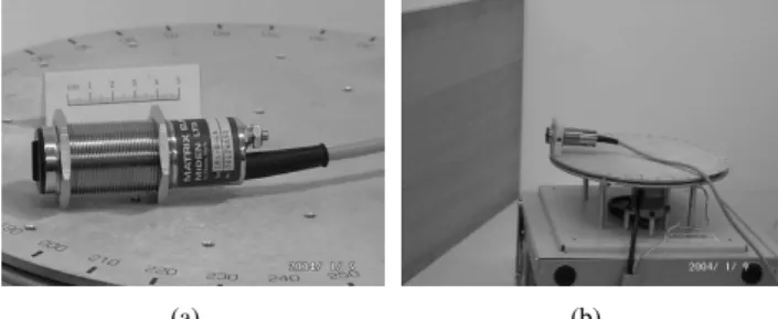
(a) (b)

Figure 1: (a) The IR sensor and (b) the experimental setup. used in door detection and mapping of openings in walls [2], as well as monitoring doors/windows of buildings and vehi-cles, and “light curtains” for protecting an area. In [3], the properties of a planar surface at a known distance were de-termined using the Phong model and the IR sensor was mod-eled as an accurate range finder for surfaces at short ranges. (A short survey on the use of infrared sensors can be found in [1]). In [4], we considered targets with different geometri-cal properties but made of the same surface material (wood). In [5], targets made of different surface materials but of the same planar geometry were differentiated. In this paper, we deal with the problem of differentiating and localizing targets whose geometry and surface properties both vary, generaliz-ing and unifygeneraliz-ing the results of [4] and [5].

2. TARGET DIFFERENTIATION AND LOCALIZATION

The IR sensor [6] used in this study [see Fig. 1(a)] consists of an emitter and detector and provides analog output voltage proportional to the measured intensity reflected off the target. The detector window is covered with an IR filter to minimize the effect of ambient light on the intensity measurements.

The targets employed are a plane, a 90◦_{corner, and a 90}◦

edge, each with a height of 120 cm. They are covered with aluminum, white cloth, and Styrofoam packaging material. Our method is based on angularly scanning each target over a certain angular range. The IR sensor is mounted on a 12 inch rotary table [7] to obtain angular scans from these targets. A photograph of the experimental setup and its schematics can be seen in Figs. 1(b) and 2, respectively. Reference data sets are collected for each target with 2.5 cm distance increments, from their nearest to their maximum observable ranges, at

θ=0◦_.

The resulting reference scans for the plane, the corner, and the edge covered with materials of different surface

properties are shown in Fig. 3. The intensity scans areθ

varia-line−of−sight sensor α target r rotary table infrared

Figure 2: Top view of the experimental setup. Both the scan

angleα and the azimuthθ are measured counter-clockwise

from the horizontal axis.

tions in both the magnitude and the basewidth of the inten-sity scans. Scans of corners covered with white cloth and Styrofoam packaging material have a triple-humped pattern (with a much smaller middle hump) corresponding to the two orthogonal constituent planes and their intersection. The in-tensity scans for corners covered with aluminum [Fig. 3(d)] have three distinct saturated humps.

For an arbitrarily located target whose intensity scan is acquired, first, we check for saturation by examining the

cen-tral intensity value of the observed scan I(α). This situation

is treated separately as will be explained later in Section 2.3. Note that a corner scan is considered saturated when its cen-tral intensity enters the saturation region, not the humps, since the former value is relevant for our method.

Two alternative approaches, employed in performing the comparisons with the reference scans, are discussed below. 2.1 Least-Squares (LS) Approach

First, we estimate the angular position of the target. As-suming the observed scan pattern is not saturated, we check whether or not it has two major humps. If so, it is a corner and we find the angular location of the corner by taking the average of the angular locations of the peaks of the two ma-jor humps of the intensity scan. If not, we find the angular location of the peak of the single hump. This angular value can be directly taken as an estimate of the angular position of the target. Alternatively, the angular position can be esti-mated by finding the center of gravity (COG) of the scan as follows: θCOG=∑ n i=1αiI(αi) ∑n i=1I(αi) (1)

Ideally, these two angular position estimates would be equal, but in practice they differ by a small amount. We consider the use of both alternatives when tabulating our results. From now on, we refer to either estimate as the “center angle” of the scan.

Plots of the intensity at the center angle of each scan in Fig. 3 as a function of the distance at which that scan was obtained, play an important role in our method. Fig. 4 shows these plots for the intensity value at the COG for planes, cor-ners, and edges.

In this approach, we compare the intensity scan of the observed target with the nine reference scans by computing their LS differences after aligning their centers with each other. The mean-square difference between the observed scan and the nine scans is computed as follows:

E_j=1 n n

∑

SCAN ANGLE (deg)

INTENSITY (V) (a) −90 −75 −60 −45 −30 −150 015 30 45 60 75 90 2 4 6 8 10 12

SCAN ANGLE (deg)

INTENSITY (V) (b) −90 −75 −60 −45 −30 −15015 30 45 60 75 90 0 2 4 6 8 10 12

SCAN ANGLE (deg)

INTENSITY (V) (c) −120−100 −80 −60 −40 −200 020 40 60 80 100 120 2 4 6 8 10 12

SCAN ANGLE (deg)

INTENSITY (V) (d) −120−100 −80 −60 −40 −200 0 20 40 60 80 100 120 2 4 6 8 10 12

SCAN ANGLE (deg)

INTENSITY (V) (e) −120−100 −80 −60 −40 −200 0 20 40 60 80 100 120 2 4 6 8 10 12

SCAN ANGLE (deg)

INTENSITY (V) (f) −90 −75 −60 −45 −30 −150 015 30 45 60 75 90 2 4 6 8 10 12

SCAN ANGLE (deg)

INTENSITY (V) (g) −90 −75 −60 −45 −30 −150 015 30 45 60 75 90 2 4 6 8 10 12

SCAN ANGLE (deg)

INTENSITY (V) (h) −90 −75 −60 −45 −30 −15015 30 45 60 75 90 0 2 4 6 8 10 12

SCAN ANGLE (deg)

INTENSITY (V)

(i)

Figure 3: Intensity scans for targets at different distances: planes covered with (a) aluminum, (b) white cloth, (c) Sty-rofoam; corners covered with (d) aluminum, (e) white cloth, (f) Styrofoam; edges covered with (f) aluminum, (g) white cloth, (c) Styrofoam.

where Ij, j = 1, . . . ,9,denotes the nine scans. Here, αalign

is the angular shift that is necessary to align both patterns. The geometry-surface combination resulting in the smallest

value of Ej is declared as the observed target. Once the

ge-ometry and surface type are determined, the range can be es-timated by using linear interpolation on the appropriate curve in Fig. 4 so that the accuracy of the method is not limited by the 2.5 cm spacing used in collecting the reference scans. 2.2 Matched Filtering (MF) Approach

As an alternative, we also considered the use of MF to com-pare the observed and reference scans. The output of the matched filter is the cross-correlation between the observed intensity pattern and the jth reference scan normalized by the square root of its total energy:

yj(l) =∑pkI(αk)Ij(αk−l)

∑n

i=1[Ij(αi)]2 (3)

where l = 1, . . . ,2n − 1 and j = 1, . . . ,9. The

geometry-surface combination corresponding to the maximum cross-correlation peak is declared as the correct target type, and the angular position of the correlation peak directly provides

an estimate ofθ. Then, the distance is estimated by using

0 10 20 30 40 50 60 0 2 4 6 8 10 12 DISTANCE (cm) INTENSITY (V) aluminum white cloth Styrofoam (a) 0 10 20 30 40 50 60 0 2 4 6 8 10 12 DISTANCE (cm) INTENSITY (V) aluminum white cloth Styrofoam (b) 0 10 20 30 40 50 60 0 2 4 6 8 10 12 DISTANCE (cm) INTENSITY (V) aluminum white cloth Styrofoam (c)

Figure 4: Central intensity (COG) versus distance curves for different targets: (a) plane; (b) corner; (c) edge.

linear interpolation on the appropriate curve in Fig. 4 using

the intensity value at theθestimate.

2.3 Saturated Scans

If saturation is detected in the observed scan, special treat-ment is necessary. Comparisons are made between the ob-served scan and all the saturated reference scans. The range estimate of the target is taken as the distance corresponding to the scan resulting in the minimum mean-square difference in the LS approach and the distance corresponding to the best matching scan for the MF approach.

3. EXPERIMENTAL VERIFICATION AND DISCUSSION

In this section, we experimentally verify the proposed method by situating targets at randomly selected distances r

and azimuth anglesθand collecting a total of 194 test scans.

The targets are randomly located at azimuth angles varying

from –45◦ _{to 45}◦ _{from their nearest to their maximum}

ob-servable ranges in Fig. 3.

The results of LS based target differentiation are dis-played in Table 1, which gives the results obtained using the maximum intensity (or the middle-of-two-maxima inten-sity for corner) values (numbers before the parentheses) and those obtained using the intensity value at the COG of the scans (numbers in the parentheses). The average accuracy over all target types can be found by summing the correct de-cisions given along the diagonal of the confusion matrix and dividing this sum by the total number of test trials (194). The same average correct classification rate is achieved by using the maximum and the COG variations of the LS approach, which is 77%.

MF differentiation results are presented in Table 2. The average accuracy of differentiation over all target types is 80%, which is better than that obtained with the LS approach. Planes and corners covered with aluminum are correctly classified with all the approaches employed due to their dis-tinctive features. Planes of different surface properties are better classified than the others, with a correct differentiation rate of 91% for the MF approach. For corners, the highest correct differentiation rate of 83% is achieved with the COG variation of the LS approach. The greatest difficulty is en-countered in the differentiation of edges of different surfaces, which have the most similar intensity patterns. The highest correct differentiation rate of 60% for edges is achieved with the maximum intensity variation of the LS approach. Taken separately, the geometry and surface type of targets can be correctly classified with rates of 99% and 81%, which shows that the geometrical properties of the targets are more distinc-tive than their surface properties, and surface determination is the limiting factor.

The average absolute position estimation errors for the different approaches are presented in Table 3 for all test tar-gets. Using the maximum and COG variations of the LS ap-proach, the target ranges are estimated with average absolute range errors of 1.8 and 1.7 cm, respectively. MF results in an average absolute range error of 1.5 cm, which is better than the LS approach. The greatest contribution to the range errors comes from targets which are incorrectly differenti-ated and/or whose intensity scans are saturdifferenti-ated. If we aver-age over only correctly differentiated targets (regardless of whether they lead to saturation), the average absolute range

Table 1: Confusion matrix: least-squares (AL: aluminum, WC: white cloth, ST: Styrofoam, P: plane, C: corner, E: edge). d e t e c t e d P C E AL WC ST AL WC ST AL WC ST AL 24(24) – – – – – – – – a P WC – 25(25) 4(4) – – – – – – c ST – 9(9) 20(20) – – – – – – t AL – – – 22(22) – – – – – u C WC – – – – 10(13) 12(9) – – – a ST – – – – (2) 20(18) – – – l AL – – (1) – – – 9(7) – 1(2) E WC – – – – – – – 11(14) 9(6) ST – (1) 1(1) – – – – 8(10) 9(6)

Table 2: Confusion matrix: matched filter. d e t e c t e d P C E AL WC ST AL WC ST AL WC ST AL 24 – – – – – – – – a P WC – 27 2 – – – – – – c ST – 5 24 – – – – – – t AL – – – 22 – – – – – u C WC – – – – 14 8 – – – a ST – – – – 4 16 – – – l AL – – – – – – 9 1 – E WC – – – – – – – 11 9 ST – – 2 – – – – 8 8

errors are reduced to 1.2, 1.0, and 0.7 cm for the maximum and COG variations of the LS and the MF approaches, re-spectively. As for azimuth estimation, the respective average absolute errors for the maximum and COG variations of the

LS and the MF approaches are 1.6◦_{, 1.5}◦

,and 1.1

◦_{, with MF}

resulting in the smallest error. When we average over only correctly differentiated targets, these errors are reduced to

1.5◦_{, 1.2}◦

,and 0.9

◦_.

To explore the boundaries of system performance and to assess the robustness of the system, we also tested the sys-tem with targets of either unfamiliar geometry, unfamiliar surface, or both, whose scans are not included in the refer-ence data sets. Therefore, these targets are new to the system. First, tests were done for planes, corners, and edges covered with five new surfaces: brown, violet, black, and white pa-per, and wood. Planes are classified as planes 100% of the time using both variations of the LS method and 99.3% of the time using the MF approach. Corners are classified as corners 100% of the time using any of the three approaches. Edges are correctly classified 89.1% of the time using the maximum variation of the LS approach, 88.2% of the time using the COG variation of the LS approach, and 87.3% of the time using the MF approach. In these tests, no target type is mistakenly classified as a corner due to the unique charac-teristics of the corner scans. Similarly, corners of the preced-Table 3: Absolute position estimation errors for all targets.

P C E avg. method AL WC ST AL WC ST AL WC ST error LS-max r(cm) 2.2 2.3 1.0 2.1 0.8 0.5 2.4 1.9 2.7 1.8 θ(deg) 0.9 2.3 0.8 2.4 1.7 1.3 1.1 2.0 1.7 1.6 LS-COG r(cm) 2.2 0.6 1.0 2.1 0.6 0.6 3.8 1.4 3.2 1.7 θ(deg) 0.9 1.0 0.8 2.4 1.4 1.1 1.2 2.2 2.3 1.5 MF r(cm) 1.7 0.5 0.7 1.5 0.6 0.6 2.2 1.7 4.2 1.5 θ(deg) 0.8 0.9 0.7 1.0 1.1 1.0 1.1 2.6 0.9 1.1

−90 −75 −60 −45 −30 −150 0 15 30 45 60 75 90 2 4 6 8 10 12 INTENSITY (V)

SCAN ANGLE (deg)

(a) −90 −75 −60 −45 −30 −150 0 15 30 45 60 75 90 2 4 6 8 10 12 INTENSITY (V)

SCAN ANGLE (deg)

(b)

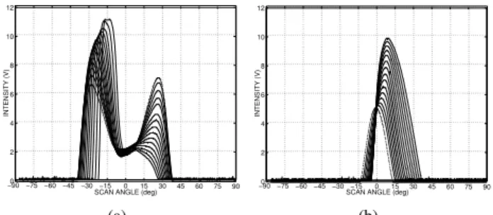
Figure 5: Intensity scans for a wooden (a) corner at 65 cm,

(b) edge at 35 cm for orientations between 0◦_{and 35}◦_with

2.5◦_{increments. The curves with the dotted lines indicate 0}◦

orientation.

ing five surfaces are never classified as planes or edges. The position errors are comparable or slightly larger than before. We also tested the system with cylinders, which were not among the three geometries in the original data sets, with the same surface types as used in the reference data sets and dif-ferent surface types (see Ref. [1] for detailed results). Cylin-ders are most likely to be classified as edges. In these two cases, average range estimation error increases to about 9– 11 cm, but the azimuth error is of the same order of magni-tude as before, since our azimuth estimation method is inde-pendent of target type.

In the remainder of this section, we discuss the effect of varying the orientation of the targets from their head-on po-sitions. Varying the orientation for planes and cylinders does not make any difference since a complete scan is acquired. Change of orientation will make a difference when the target geometry is a corner or an edge, leading to scans not exist-ing in the reference set. Unlike with the case of planes and cylinders, varying the orientation of corners and edges leads to asymmetric scans. If the scan is symmetric, it is either

a plane or a cylinder, or a corner or an edge with nearly 0◦

orientation, and the described algorithm can handle it. If the scan is asymmetric, we know that the target is either a cor-ner or an edge with nonzero orientation. While it is possible to deal with this case by extending the reference set to in-clude targets with nonzero orientation, the introduction of a simple rule allows us to handle such cases with only minor modification of the already presented algorithm. We can de-termine whether the asymmetric scan comes from a corner or an edge by checking whether or not it has two humps. Thus, even with arbitrary orientations, the target geometry can be determined. Furthermore, we observe that variations in ori-entation have very little effect on the central intensity of the asymmetric scans (see Fig. 5). This means that the central intensity value can be used to determine the distance in the same manner as before by using linear interpolation on the central intensity versus distance curves for a particular target type.

To demonstrate this, we performed additional experi-ments with corners and edges. These targets were placed at random orientation angles at randomly selected distances. A total of 100 test scans were collected. Using the orientation-invariant approach already described, 100% correct differen-tiation and absolute mean range errors of 1.02 and 1.47 cm for corners and edges were achieved.

We also tested the case where reference scans corre-sponding to different orientations are acquired. Reference data sets were collected for both targets with 5 cm distance

increments atθ=0◦_{, where the orientation of the targets are}

varied between –35◦_{to 35}◦_{with 2.5}◦_{increments. A total of}

489 reference scans were collected. For each test scan, the best-fitting reference scan was found by MF. This method also resulted in 100% correct differentiation rate. Absolute mean range and orientation errors for corners and edges were

1.13 and 1.26 cm and 4.48◦_{and 5.53}◦_.

4. CONCLUSION

In this study, differentiation and localization of commonly encountered indoor features or targets such as planes, cor-ners, and edges with different surfaces was achieved using an inexpensive IR sensor. Different approaches were compared in terms of differentiation and localization accuracy. The MF approach in general gave better results for both tasks. The robustness of the methods was investigated by presenting the system with targets of either unfamiliar geometry, unfamiliar surface type, or both.

Current and future work involves designing a more intel-ligent system whose operating range is adjustable based on the return signal intensity. This will eliminate saturation and allow the system to accurately and faster differentiate and localize targets over a wider operating range. We are also working on the differentiation of targets through the use of artificial neural networks in order to improve the accuracy. Parametric modeling and representation of intensity scans of different geometries (such as corner, edge, and cylinder) as in [8] is also being considered to employ the proposed ap-proach in the simultaneous determination of the geometry and the surface type of targets.

REFERENCES

[1] T. Aytac¸ and B. Barshan, “Simultaneous extraction of geometry and surface properties of targets using simple infrared sensors,” Opt. Eng., vol. 43, pp. 2437–2447, Oct. 2004.

[2] A. M. Flynn, “Combining sonar and infrared sensors for mobile robot navigation,” Int. J. Robot. Res., vol. 7, pp. 5–14, Dec. 1988.

[3] P. M. Novotny and N. J. Ferrier, “Using infrared sen-sors and the Phong illumination model to measure distances,” in Proc. ICRA, Detroit, MI, May 1999, pp. 1644–1649.

[4] T. Aytac¸ and B. Barshan, “Differentiation and localiza-tion of targets using infrared sensors,” Opt. Commun., vol. 210, pp. 25–35, Sep. 2002.

[5] B. Barshan and T. Aytac¸, “Position-invariant surface recognition and localization using infrared sensors,”

Opt. Eng., vol. 42, pp. 3589–3594, Dec. 2003.

[6] Matrix Elektronik, AG, Kirchweg 24 CH-5422 Oberehrendingen, Switzerland, IRS-U-4A Proximity

Switch Datasheet, 1995.

[7] Arrick Robotics, P.O. Box 1574, Hurst, Texas, 76053 URL: www.robotics.com/rt12.html, RT-12 Rotary

Po-sitioning Table, 2002.

[8] T. Aytac¸ and B. Barshan, “Surface recognition by para-metric modeling of infrared intensity signals,” in Proc.