Jm Z’İÎE-SIS s m g l:: -· -·’ G'O? y - ":v ■*’· * · '■•“'I*' *■· Q 3 2 S . S
. 6 5 7
/ 3 3 3
A THESIS
SUBMITTED TO THE DEPARTMENT OF COMPUTER
ENGINEERING AND INFORMATION SCIENCE AND THE INSTITUTE OF ENGINEERING AND SCIENCE
OF BILKENT UNIVERSITY
IN PARTIAL FULFILLMENT OF THE REQUIREMENTS
FOR THE DEGREE OF
MASTER OF SCIENCE
By
izzet Şirin
August, 1993
... ....'/''îtI certify that I have read this thesis and that in my opinion it is fully adequate, in scope and in quality, as a thesis for the degree of Master of Science.
Asst. Prof. HaftljAltay Güvenir (Advisor)
I certify that I have read this thesis and that in my opinion it is fully adequate, in scope and in quality, as a thesis for the degree of Master of Science.
Assoc. Prof. Varol Akman
I certify that I have read this thesis and that in my opinion it is fully adequate, in scope and in quality, as a thesis for the degree of Master of Science.
^j^;;:^sst. PiWT Kemal Oflazer
Approved for the Institute of Engineering and Science:
Prof. Mehmet Banaj^ Director of the Institute
LEARNING WITH FEATURE PARTITIONS
İzzet Şirin
M.S. in Computer Engineering and Information Science
Advisor: Asst, Prof. Halil Altay Güvenir
August, 1993
This thesis presents a new methodology of learning from examples, based on
feature partitioning. Classification by Feature Partitioning (CFP) is a particu
lar implementation of this technique, which is an inductive, incremental, and supervised learning method. Learning in CFP is accomplished by storing the objects separately in each feature dimension as disjoint partitions of values. A partition, a basic unit of representation which is initially a point in the feature dimension, is expanded through generalization. The CFP algorithm special izes a partition by subdividing it into two subpartitions. Theoretical (with respect to PAC-model) and empirical evaluation of the CFP is presented and compared with some other similar techniques.
Keywords: Machine learning, inductive learning, incremental learning, super
vised learning, feature partitioning.
OZNITELIK
b ö l ü n t ü l e r i
İLE ÖĞRENME
izzet Şirin
Bilgisayar ve Enformatik Mühendisliği, Yüksek Lisans
Danışman: Y. Doç. Dr. Halil Altay Güvenir
Ağustos, 1993
Bu çalışmada öznitelik bölünmesine dayalı yeni bir mekanik öğrenme yöntemi sunulmuştur. Bu yöntem kullanılarak bir sınıflama algoritması olan Öznitelik
Bölüntüleri ile Sınıflayıct C FP’nin yazılımı hazırlanmıştır. CFP algoritması
mekanik öğrenmeyi tümevarım ve artırımlı öğrenme yöntemlerini kullanarak sağlar. CFP algoritmasında bölütü elemanları temel gösterim unsurlarıdır. Başlangıçta bölüntü elemanları bir boyutlu uzayda bir noktayı ifade ederken, zaman içinde bu elemanlar genişleyerek bir aralığı ifade ederler. Bölüntü el emanları parçalanarak özelleştirilirler. CFP algoritmasının kuramsal analizi
yaklaşık olarak doğru kuramına (PAC-model) göre yapılmıştır ve benzer sis
temlerle uygulama sonuçları karşılaştırılmıştır.
Anahtar Sözcükler: Mekanik öğrenme, tümevarımsal öğrenme, artırımsal
öğrenme, denetimli öğrenme, öznitelik bölüntüleme.
I would like to express my deep gratitude to my supervisor Asst. Prof. Halil Altay Güvenir for his guidance, suggestions, and invaluable encouragement throughout the development of this thesis.
I would also like to thank Assoc. Prof. Varol Akman and Asst. Prof. Kemal Oflazer for reading and commenting on the thesis.
I owe special thanks to Prof. Mehmet Baray for providing a pleasant envi ronment for study.
I am grateful to the members of my family for their infinite moral support and patience that they have sliown, particularly in times I was not with them.
1 Introduction 1
2 Previous M odels 6
2.1 Symbolic M o d e ls ... 6
2.1.1 Explanation-Based Learning ( E B L ) ... 7
2.1.2 Instance-Based L e a rn in g ... 8
2.1.3 Nested Generalized E xem plars... 10
2.1.4 K Nearest Neighbors (KNN) Algorithm 12 2.1.5 Decision T r e e ... 12
2.1.6 The PLSl A lg o rith m ... 13
2.2 Subsymbolic M o d e l s ... 14
2.2.1 Connectionist P a r a d ig m ... 14
2.2.2 Genetic A lgorithm s... 15
2.3 Comparison of CFP with Other M odels... 17
3 Learning w ith Feature Partitions 21 3.1 The CFP A lg o r ith m ... 21
3.2 A noise tolerant version of the C F P ... 30 vi
3.3 Parallelization of the C F P ... 31
3.4 The GA-CFP A lg o rith m ... 31
3.5 Limitations of the C F P ... 36
3.5.1 Nonrectangular Concept D escriptions... 36
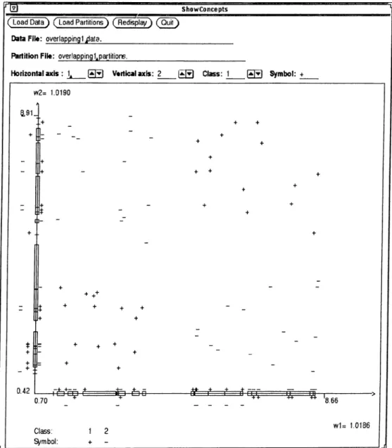
3.5.2 Overlapping Concept Description P r o je c tio n s ... 37
3.5.3 Domain Dependent Parameters of the C F P ...40
4 Evaluation of the CFP 42 4.1 Theoretical Evaluation of the CFP ... 42
4.2 Empirical Evaluation of the C F P ... 47
4.2.1 Testing M ethodology... 48
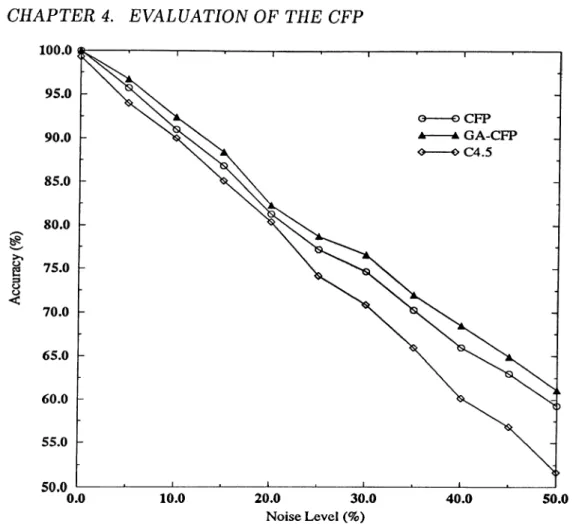
4.2.2 Experiments with Artificial Data S e ts ... 49
4.2.2.1 Changing Domain C haracteristics... 50
4.2.2.2 Sensitivity of the CFP to its Domain Depen dent P a r a m e te r s ... 55
4.2.3 Experiments with Real-world Data S e ts... 63
5 Conclusion 75
6 A ppend ix 82
1.1 Classification of exemplar-based learning alg o rith m s... 4
2.1 A skeleton of a simple genetic a lg o r ith m ... 16
3.1 Partitioning of a feature d im e n s io n ... 22
3.2 Training algorithm of the C F P ... 24
3.3 The Prediction process of CFP ... 25
3.4 The Classification process of C F P ... 26
3.5 Updating a feature p a rtitio n ... 27
3.6 An example concept description in a domain with two features . 28 3.7 Parameter encoding schemes of the G A -C F P ... 32
3.8 The CFP fitness function of the G A -C F P ... 34
3.9 Learning curve of domain dependent p aram eters... 35
3.10 An example of nonrectangular concept d e s c rip tio n s ... 37
3.11 An example of nested concept d escrip tio n s... 38
3.12 An example of overlapping projection of concept descriptions . . 39
3.13 An example of partially overlapping projection of concept de scriptions ... 41
4.1 Comparison of (GA-)CFP, and C4.5 in terms of accuracy, on a noisy d o m a i n ... 51 4.2 Comparison of (GA-)CFP, and C4.5 in terms of accuracy, on a
domain that contains unknown attribute v a l u e s ... 52 4.3 Comparison of (GA-)CFP, and C4.5 in terms of accuracy on
domains with many irrelevant a t t r i b u t e s ... 54 4.4 Effects of the generalization limit to the accuracy of the CFP . . 56 4.5 Effects of the generalization limit to the memory requirement of
the C F P ... 56 4.6 Effects of the weight adjustment rate to the accuracy of the CFP 57 4.7 Effects of the confidence threshold to the accuracy of the CFP . 58 4.8 Effects of the confidence threshold to the memory requirement
of the CFP ... 59 4.9 Effects of the confidence threshold to the accuracy of the CFP,
on noisy d o m a in s ... 60 4.10 Effects of the confidence threshold to the memory requirement
of the CFP, on noisy d o m a in s ... 61 4.11 Effects of the confidence threshold to the accuracy of the CFP,
on a domain with many irrelevant a ttr ib u te s ... 62 4.12 Effects of the confidence threshold to the memory requirement
of the CFP, on a domain with many irrelevant attributes . . . . 62 4.13 2-D view of the iris data: Sepal length vs. Sepal w i d t h ...65 4.14 2-D view of the iris data: Petal length vs. Petal width ... 66
4.1 Success rates for iris flowers ( % ) ... 64
4.2 Success rates for breast cancer data (%) ... 65
4.3 Success rates for Hungarian heart disease data (%) ...67
4.4 Success rates for Cleveland heart disease data ( % ) ... 68
4.5 Success rates for waveform data (% )... 68
4.6 Success rates for congressional voting database ( % ) ...69
4.7 Success rates for glass data ( % ) ... 70
4.8 Success rates for Pima Indians diabetes database ( % ) ... 70
4.9 Success rates for ionosphere database (%) 71
4.10 Success rates for liver disorders database ( % )... 72
4.11 Success rates for wine classification data ( % ) ... 72
4.12 Success rates for thyroid data ( % ) ... 73
AI Artificial Intelligence.
CFP Classification by feature partitioning. a· Label of the fth class.
C4 Decision tree algorithm. C4.5 Decision tree algorithm.
C (n ,r) Number of combinations of r object out of n.
C T Confidence threshold parameter of the CFP.
D Probability distribution defined on the instance space
D f Generalization limit for feature / in CFP. 3-DNF Third disjunctive normal form.
E An example. e An example.
^class Class of example e.
Feature value of example e.
Rn Euclidean n-dimensional space.
EACH Exemplar-aided constructor of hyperrectangles. EBG Explanation-based generalization.
EBL Explanation-based learning. GA Genetic algorithm.
GA-CFP Hybrid CFP algorithm.
(GA)-CFP GA-CFP and CFP algorithms. GA-WKNN Hybrid WKNN algorithm.
h Hypothesis.
H Hyperrectangle.
^Slower Lower boundary of
Hk-^kupper Upper boundary of
IBL Instance-based learning. ID3 Decision tree algorithm. KA Knowledge acquisition. KBS Knowledge-based Systems. KNN К Nearest neighbors algorithm. In Natural logarithm,
log Logarithm in base two.
M, m The number of training examples.
ML Machine learning.
NGE Nested generalized exemplars. PAG Probably approximately correct. PLSl Probabilistic learning algorithm.
votec Voting power of class c.
WKNN Weighted К nearest neighbors algorithm.
wj Weight of feature / .
u)//* Weight of hyperrectangle k.
A Weight adjustment rate of the CFP algorithm.
6 Confidence parameter of the PAC-model. £ Error parameter of the PAC-model.
7 Probability of distance between to adjacent point is greater than e. II Absolute value.
{} Comment in the algorithm of CFP.
[x, y\ Closed interval in which boundaries are x and y.
[x] The smallest integer number greater than or equal to x.
X Multiplication. / Division.
In tro d u ctio n
The development of knowledge-based systems (KBS) is a difficult and often time consuming task. The acquisition of the knowledge necessary to perform a certain task (usually through a series of acquisition sessions with a domain ex pert) is considered as one of the main bottlenecks in building KBS. Knowledge acquisition (KA) and machine learning (ML) have been closely linked by their common application field, namely building up knowledge bases for KBS. Learn ing and KA can be viewed as two processes that construct a model of a task domain, including the systematic patterns of interaction of an agent situated in a task environment. Learning of an agent involves both learning to solve new problems and learning better ways to solve previously solved problems. Carbonell describes machine learning eis follows [6]:
Perhaps the tenacity of ML researchers in light of the undisputed difficulty of their ultimate objectives, and in light of early disap pointments, is best explained by the very nature of the learning process. The ability to learn, to adapt, to modify behavior is an inalienable component of human intelligence.
The motivation for applying ML techniques to real-world tasks is strong. ML offers a technology for assisting in the KA process. There is a potential for automatically discovering new knowledge in the available on-line databases which are too large for humans to manually sift through. Furthermore, the ability of computers to automatically adapt to changing expertise would offer huge benefits for the maintenance and evolution of expert systems.
The success of a learning system is highly related to the ability to cope with noisy and incomplete data, an adequate knowledge representation scheme, hav ing low learning and sample complexities, and the effectiveness of the learned knowledge [24].
Tradeoffs between learning and programming can also be examined in terms of their relative utilities. Computer time is now very cheap, whereas human labor is becoming increasingly expensive. This suggests that learning could have an immediate economic edge over manual methods of programming the same information. Of course, there are many situations in which the potential benefit of developing a knowledge base far exceeds the cost of its capture.
Evaluating the utility of programmed and learned knowledge cannot stop with a simple human level of effort analysis. However, computational efficiency of algorithms and the representations they use dramatically affect both the size of the computers that are required and the size of the problems one can solve.
The most widely studied method for symbolic learning is one of inducing a general concept description from a sequence of instances of the concept and (usually) known counterexamples of the concept. The task is to build a con cept description from which all previous positive instances can be rederived by universal instantiation but none of the previous negative instance (counterex ample) can be rederived by the same process [6].
Learning from examples has been one of the primary paradigms of ML re search since the early days of Artificial Intelligence (AI). Many researchers have observed and documented the fact that human problem solving performance improves with experience. In some domains, the principal source of expertise seems to be a memory to hold a large number of important examples. For example, in chess human experts seem to have a memory of roughly 50,000 to 70,000 specific patterns. The attempts to build an intelligent (i.e., at the level of human) system have often faced the problem of memory for too many spe cific patterns. Researchers expect to solve this difficulty by building machines that can learn. This reasoning has motivated many machine learning projects [31].
Inductive learning is a process of acquiring knowledge by drawing inductive inference from teacher (or environment) provided facts. Such a process involves operations of generalizing, specializing, transforming, correcting and refining knowledge representations. There are several different methods by which a
human (or machine) can acquire knowledge, such as rote learning (or learning by being programmed), learning from instruction (or learning by being told), learning from teacher provided examples (concept acquisition), and learning by observing the environment and making discoveries (learning from observation and discovery).
Learning a concept usually means to learn its description, i.e., a relation between the name of the concept and a given set of features. Several differ ent representation techniques have been used to describe concepts for super vised learning tasks. One of the widely used representation technique is the
exemplar-based representation. The representation of the concepts learned by
the exemplar-based learning techniques stores only specific examples that are representatives of other several similar instances. Exemplar-based learning was originally proposed as a model of human learning by Medin and Schaffer [25].
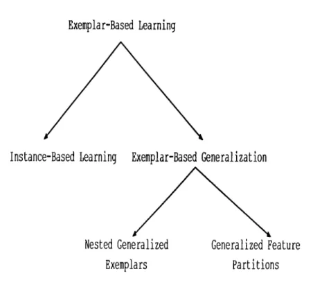
There are many different exemplar-based learning models in the literature (see Fig. 1.1). All of these models share the property that they use verbatim examples as the basis of learning. For example, instance-based learning [1] retains examples in memory as points, and never changes them. The only decisions to be made are what points to store and how to measure similarity. Aha, Kibler, and Albert [1] have created several variants of this model, and they are experimenting with how far they can go with strict point-storage model. Another example is the nested-generalized exemplars model of Salzberg [34]. This model changes the point storage model of the instance-based learning and retains examples in the memory as axis-parallel hyperrectangles.
Previous implementation of the exemplar-based models usually extend the nearest neighbor algorithm in which some kind of similarity (or distance) metric is used for prediction. Hence, prediction complexity of such algorithms is proportional to the number of instances (or objects) stored.
This thesis presents another form of exemplar-based learning, based on the representation of feature partitioning. CFP is a particular implementation of the feature partitioning technique. The CFP partitions each feature into seg ments corresponding to concepts. Therefore, the concept description learned by the CFP is a collection of feature partitions. In other words, the CFP learns a projection of the concept on each feature dimension. The CFP algorithm makes several significant improvements over other exemplar-based learning al gorithms, where the examples are stored in memory without any change in
Exemplar-Based Learning
Instance-Based Learning Exemplar-Based Generalization
Nested Generalized
Exemplars
Generalized Feature
Partitions
Figure 1.1. Classification of exemplar-based learning algorithms
the representation. For example, IBL algorithms learn a set of instances (a representative subset of all training examples), EACH (Exemplar-Aided Con structor of Hyperrectangles) learns a set of hyperrectangles of the examples. On the other hand, the CFP algorithm stores the instances as factored out by their feature values.
Since the CFP learns projections of the concepts, it does not use any similar ity (or distance) metric for prediction. Each feature contributes the prediction process by its local knowledge. Final prediction is based on a voting among the predictions of the features. Since a feature partition can be represented by a sorted list of line segments, the prediction by a feature is simply a search for the partition corresponding to the instance on that sorted list. Thei'efore, the CFP algorithm significantly reduces the prediction complexity, over other exemplar-based techniques. The power of a feature in the voting process is determined by the weight of that feature. Assigning variable weights to the features enables the CFP to determine the importance of each feature to re flect its relevance for classification. This scheme allows smooth performance degradation when data set contains irrelevant features.
The issue of unknown attribute values is an unfortunate fact of real-world data sets, that data often contain missing attribute values. Most of the learning
systems, usually overcome this problem by either filling in missing attribute values (with most probable value or a value determined by exploiting inter relationships among the values of different attributes) or by looking at the probability distribution of known values of that attribute. Most common ap proaches are compared in Quinlan [29], leading to a general conclusion that some approaches are clearly inferior but no one approach is uniformly superior to others. In contrast, CFP solves this problem very naturally. Since CFP treats each attribute value separately, in the case of an unknown attribute value, it simply leaves the partitioning of that feature intact. That is the unknown values of an instance are ignored while only the known values are used.
In the next chapter some of the previous models are presented and several different properties of the learning method are explored. The precise details of the CFP algorithm are described in Chapter 3. The process of partitioning of a feature dimension is illustrated with an example, and several extensions to the CFP algorithm are described. Chapter 4 presents theoretical and em pirical evaluation of the CFP algorithm. A theoretical analysis of the CFP algorithm with respect to PAC-learning theory is presented. Performance of the CFP on artificially generated data sets and comparisons with other similar techniques on real-world data sets are also presented. The final chapter dis cusses the applicability of the CFP and concludes with a general evaluation of the algorithm.
P re v io u s M o d els
It is well known that two major directions of AI research, symbolic and suhsym-
holic models, exhibit their strengths and weakness in an almost complementary
ways. While symbolic models are good in high-level reasoning, they are weak in handling imprecise and uncertain knowledge and data. On the other hand subsymbolic models are good in lower-level reasoning such as imprecise classi fication and recognition problems. However, they are not good in higher-level reasoning. Nevertheless, both models contribute important insight to our un derstanding of intelligent systems. Fortunately, over the last few years these two approaches have become less separate, and there has been an increasing amount of research that can be considered a hybrid of the two approaches [4, 13, 37].
2.1
S y m b o lic M o d els
Two of the main types of learning from examples in the history of AI research are concept learning and explanation-based learning.
Concept Learning: Concept learning tackles the problem of learning con
cept definitions. A definition is usually a formal description in terms of a set of attribute-value pairs, often called features. More recently, approaches using decision trees, connectionist architectures, representative instances, and hyper rectangles (exemplar-based learning) have appeared in the literature. These approaches construct concept description by examining a series of examples.
each of which is categorized as either an example of the concept or a counterex ample. A learning system can refine its concept description until it matches the correct description.
Exemplar-based learning is a kind of concept learning in which the concept definition is constructed from the examples themselves, using the same repre sentation language. In the instance-based learning in fact, the examples are the concept (no generalizations are formed). Like other concept learning theories, exemplar-based learning requires little or no domain specific knowledge.
2.1.1
E x p la n a tio n -B a sed L earning (E B L )
Dejong and Mooney [9] present a general technique for learning by generalizing explanations. They discuss the differences of their model with the Explanation-
Based Generalization (EBG) [21]. The border term EBL better describes the
approach than does EBG. It seems both possible and desirable to apply the approach to concept refinement (i.e., specialization) as well as concept gener alization. The explanation-based approach uses domain-specific knowledge as much as possible. This approach has been more commonly used in ML. An explanation consists of an inference chain (which may be a proof, but may also be mei'ely plausible reasoning) that identifies one or more of these variables as the cause of the wrong prediction. This subset of variables is linked by the inference chain to correct the prediction. Once the variables have been identi fied, the system must revise its prediction model in some way to reflect the fact that a particular set of variables is now associated with the new prediction.
The difficult part of the EBL is the identification of the proper set of the variables that cause the wrong prediction. The number of possible subsets of the variables increases exponentially with the number of variables, so this is intractable. Hence, EBL systems use domain-specific knowledge to select, from a large set of possible explanations, a few plausible explanations. The domain knowledge is used to construct a proof that specific variables caused the wrong prediction. The knowledge that must be provided includes detailed knowledge about how each variable affect the prediction, and how input variables interact. Another goal of the EBL methods is that they attem pt to construct as concise a description as possible of the input examples.
The generalization method described in Mitchell [21] EBG, must be pro vided with the following information:
1. Goal concept: A definition of the concept to be learned in terms of high- level or functional properties which are not directly available in the rep resentation of an example.
2. Training example: A representation of a specific example of the concept in terms of lower level features.
3. Domain theory: A set of inference rules and facts sufficient for proving that a training example meet the high-level definition of the concept. 4. Operationality criterion: A specification of how a definition of a concept
must be represented so that the concept can be efficiently recognized.
Given this information, EBG constructs an explanation of why the training example satisfies the goal concept by using the inference rules in the domain theory. This explanation takes the form of a proof tree composed of Horn- clause inference rules which proves that the training example is a member of the concept.
2.1.2
In sta n ce-B a sed Learning
The primary output of IBL algorithms is a concept description, which is a function that maps instances to concepts. Instance-based learning technique [1], has been implemented in three different algorithms, namely IB l, IB2, and IB3. IBl stores all the training instances, IB2 stores only the instances for which the prediction was wrong. Neither IBl nor IB2 remove any instance from concept description after it had been stored. IB3 employs a significance test (i.e., acceptable or significantly poor) to determine which instances are good classifiers and which ones are believed to be noisy.
An instance-based concept description includes a set of stored instances and some information concerning their past performance during the training pro cess, e.g., the number of correct and incorrect classification predictions. The final set of instances can change after each training process. However, IBL algorithms do not construct intensional concept descriptions Instead, concept
descriptions are determined by how IBL algorithm’s similarity and classifi
cation functions use the current set of saved instances. The similarity and
classification functions determine how the set of saved instances in the concept description are used to predict values for the category attribute. Therefore, IBL concept descriptions contain these two functions along with the set of stored instances.
Three components of IBL algorithms are:
1. Similarity function: computes the similarity between an instance and instances in concept description.
2. Classification function: yields the classification for an instance by using the result of the similarity function and performance record of the concept description.
3. Concept description updater, maintains records on classification perfor mance and decides which instances should be included in the concept description.
IBL algorithms assume that, instances that have high similarity values ac cording to the similarity function, have similar classifications. This leads to their local bias for classifying novel instances according to their most simi lar neighbor’s classification. They also assume that, without prior knowledge, attributes will have equal relevance for classification decisions (i.e. each fea ture has equal weight in similarity function). This assumption may lead to significant performance degradation if the data set contains many irrelevant features.
IB3 is the noise tolerant version of the IBL algorithms. It employs wait
and see evidence gathering method to determine which of the saved instances
are expected to perform well during classification. In all IBL algorithms, the similarity between instances x and y is computed as:
sim ilarity {x.,y) = — - y^y
¿=1
IB3 maintains a classification record (i.e. number of correct and incorrect classification attempts) with each saved instance. A classification record sum marizes an instances’s classification performance on subsequently presented
training instances and suggests how it will perform in the future. IB3 employs a significance test (i.e. acceptable and significantly poor) to determine which instances are good classifiers and which ones are believed to be noisy. IB3 accepts an instance if its classification accuracy is significantly greater than its class’s observed frequency and removes an instance from concept description if its accuracy is significantly less. Confidence intervals are used to determine whether an instance is acceptable, mediocre, or noisy. Confidence intervals are constructed around both the current classification accuracy of the instance and current observed relative frequency of its class.
2.1.3
N e s te d G en eralized E xem p lars
In Nested Generalized Exemplars (NGE) theory, learning is accomplished by storing objects in Euclidean ?z-space, jE", as hyperrectangles [34]. NGE is also a variation of exemplar-based learning. In the simplest form of the exemplar- based learning, every example is stored in memory, with no change in represen tation (or without generalization), as in IBl algorithm presented above. NGE adds generalization on top of the simple exemplar-based learning. It adopts the position that exemplars, once stored, should be generalized. The learner compares a new example to those it has seen before and finds the most simi lar, according to a similarity metric, which is inversely related to the distance metric (Euclidean distance in n-space). The term exemplar (or hyperrectangle) is used to denote an example stored in memory. Over time, exemplars may be modified (due to generalization) from their original forms. This is similar to the generalizations of partitions in the CEP algorithm.
Once a theory moves from a symbolic space to Euclidean space, it becomes possible to nest one generalization inside the other. Its generalizations, which take the form of hyperrectangles in can be nested to an arbitrary depth, where inner rectangles act as exceptions to the outer ones.
EACH (Exemplar-Aided Constructor of Hyperrectangles) is a particular implementation of the NGE technique [34], where an exemplar is represented by a hyperrectangle. EACH uses numeric slots for feature values of exemplar. The generalizations in EACH take the form of hyperrectangles in Euclidean
n-space, where the space is defined by the feature values for each example.
Therefore, the generalization process simply replaces the slot values with more general values (i.e., replacing the range of values [o, 6] with another range [c.
c?], where c < a and d > b ). EACH compares the class of a new example with the most similar (shortest distance) exemplar in the memory. The distance between an example and an exemplar is computed according to the following distance function: Distance{E, Hk) =
\
difi «■=1 maxi — m in i' where Hk·. H k.ref erence: Hk .correct: ^^low.tr * k u p p e r* E: fi-E fr WHV w j,: maxi, mini: difi: hyperrectangle kthe number of reference to Hk
the number of correct prediction made by Hk lower boundary of Hk
upper boundary of Hk an example
ith feature
ith feature value of exampleE
weight of H k{H k.ref erence/Hk.cor reel) weight of fi
maximum and minimum feature values, respectively the distance between E and H on the ith dimension
difi =
E f i — - i ^ i t u p p e r E f ^ > H k upper
Hklo w e r ^ S i \ i E j , < H k lo w er 0 otherwise.
If a training example and the nearest exemplar are the same (i.e. a correct prediction has been made) the exemplar is generalized to include the new example if it is not already contained in the exemplar. However, if the closest example has a different class then that of the example, then the second closest exemplar is tried in the similar way. The idea behind the second minimum is to apply the second chance heuristic. This heuristic is useful to reduce the number of exemplars in the memory. If none the closest two exemplars has the same class as the example, then the algorithm modifies the weights of features so that the weights of the features that caused the wrong prediction is increased (in terms of distance).
2.1.4
K
N ea r est N eigh b ors (K N N ) A lg o rith m
The nearest neighbor classification algorithm is based on the idea that, given a data set of classified examples, an unclassified instance should belong to the same class as its nearest neighbors in the data set. A common extension to the nearest neighbor algorithm is to classify a new instance by looking at its
k nearest neighbors { k > 1 ). The k nearest neighbors algorithm classifies
a new instance by noting its distance from each of the stored instances and assigning the new instance to the class of the majority of its nearest neigh bors. Different ways of computing similarity or distances between instances are compared by Salzberg [33]. This algorithm can be quite effective when the attributes of the data are equally important. However, if the attributes are not equally important, performance of the algorithm degrades. Usually to solve this problem feature weights are introduced, resulting in the WKNN algox’ithm [22]. Assigning variable weights to the attributes of the instances before applying the KNN algorithm distorts the feature space, modifying the importance of each attribute to reflect its relevance for classification. In this way, closeness or similarity with respect to important attributes becomes more critical than similarity with respect to irrelevant attributes.
The GA-WKNN algorithm [22] combines the optimization capabilities of a genetic algorithm with the classification capabilities of the WKNN algorithm. The goal of the GA-WKNN algorithm is to learn an attribute weight vector which improves the WKNN classification performance. Chromosomes are vec tors of real-valued weights. A vector value is associated with each attribute and one is associated with each of the k neighbors. Thus the length of the chromosome is the number of features plus k. Another extension to the KNN is to combine simple KNN with genetic algorithms (GAs)
2.1.5
D ec isio n Tree
The decision tree is a well-known representation for classification tasks. This representation has been used in a variety of systems. Among them the most famous are ID3 [27] and its extension C4.5 [29] of Quinlan.
A decision tree can be used to classify a case by starting at the root of the tree and moving through it until a leaf is encountered. At each non-leaf
decision node, the outcome of the case for the test at the node is determined and attention shifts to the root of the subtree coi'responding to this outcome. When this process finally leads to a leaf, the class of the case is predicted to be that record at the leaf.
A decision tree is global for each attributes, in other words each non-leaf decision node may specify some test on any one of the attributes. The CFP algorithm can be seen to produce special kind of decision trees. Unlike IDS, the CFP probes each feature exactly once. An important difference between decision tree approach and other approaches mentioned above, including CFP, is that the classification performance of these systems does not depend critically on any small part of the model. In contrast, decision trees are much more susceptible to small alterations.
2.1.6
T h e P L S l A lg o rith m
Both ID3 [27] and probabilistic learning system (PLSl) [30, 31] use probabilistic criteria to specialize hypotheses, and start with a single general description and split into two or more parts. The process of splitting continues, using one attribute for each split, until some stopping criterion is satisfied.
The PLSl accepts instances of known class membership, and based on their frequency, divides the instance space into mutually exclusive regions or
probability classes. Like ID3, PLSl also uses specialization. It represents input
instances as points in a fc-dimensional space creates orthogonal hyperrectangles by inserting boundaries parallel to instance space axes. Each hyperrectangle
r is annotated with values: (1) the probability u of finding a positive example
within r, and (2) an error measure e of u. These annotated hyperrectangles (r,
u, e), called regions.! ^re like nodes of a decision tree annotated with probability
and error measures. PLSl was compared with ID3 and C4 by Rendell [31, 32]. These comparisons show that two algorithms are similar, although they differ in some striking ways. For example, the splitting criteria are different. C4 prunes its decision tree to eliminate noise, whereas PLSl faces that problem by splitting only if the statistical significance is high (and never prunes).
2.2 S u b sy m b o lic M o d els
Both symbolic and subsymbolic models contribute an important insight to our understanding of intelligent systems. Connectionist models and Genetic Algorithms (GAs) are the best known examples of subsymbolic computation. This section presents a brief description of these subsymbolic models. I will not attem pt to define precisely the essential differences between symbolic and subsymbolic approaches. This is beyond the scope of this thesis.
2.2.1
C o n n ectio n ist P arad igm
A neural network (or connectionism) is a kind of computation system in which the state of a system is represented as a numerical distribution pattern with many processing units and connections among those units. Learning by neu ral networks uses an algorithm for transforming distribution patterns, which quite different from learning based on symbolic representations. Connectionist systems have stirred a great deal of excitement for number of reasons.
1. They are novel. Connectionism seems to be a good candidate for a major new paradigm in AI where there have only been a handful of paradigms. 2. They have cognitive science potential. While connectionist neural nets
are not accurate models of neurons, they do seem brain-like and capable of modeling a substantial range of cognitive phenomena.
3. Connectionist systems have exhibited non-trivial learning. They are able to self-organize, given only examples as inputs.
4. Connectionist systems can be made fault-tolerant and error-correcting, degrading gracefully for cases not encountered previously.
5. An appropriate and scalable connectionist hardware is rapidly becoming available. This is important for applicability of the connectionist systems to the large-scale cognitive phenomena.
6. Connectionist architectures also scale well, in that modules can be inter connected rather easily. This is because message passed between modules are generally activation level, not symbolic messages.
However, there are considerable difficulties still ahead for connectionist models. Many different connectionist architectures were proposed in the litera ture. It is important to note that there are connectionist architectures beyond the simple feed-forward, single-hidden-layer neural networks. In particular, re current [10] with their feedback loops and ’’memory”, are especially appealing for application to symbolic tasks that have a sequential nature.
2.2.2
G e n e tic A lg o rith m s
Genetic algorithms (GAs) are adaptive generaie-and-test procedures derived from principles of natural population genetics. This section presents a high- level description of one formulation of genetic algorithms. GAs represents a class of adaptive search techniques that have been intensively studied in recent years. The key feature of GAs is that adaptation proceeds, not by making incremental changes to a single structure but by maintaining a population (or database) of structures from which each structure in the population has an associated fitness (goal-oriented evaluation). These fitness values are used in
competition to determine which structures are used to form new ones [19].
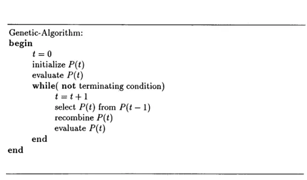
Genetic algorithms are best viewed as another tool for the designer of learn ing systems. The selection of a good feedback mechanism that facilitates the adaptive search strategy, is critical issue for the effectiveness of GAs. Detailed descriptions, of genetic algorithms, are given by Goldberg [14]. A skeleton of a simple genetic algorithm is shown in Fig. 2.1.
During iteration {generation) t, the genetic algorithm maintains a popula
tion P{t) of structures { x \ ,x l , ..., chosen from the domain of the objective function / . The initial population P(0) is usually chosen at random. The pop ulation size N remains fixed for the duration of the search. Each structure is evaluated by computing f{x\)· Usually, the term trial is used for each such evaluation. This provides a measure of fitness of the evaluated structure for the given problem. When each structure in the population has been evaluated, a new population of structures is formed in two steps.
First, structures in the current population are selected to reproduce on the basis of their relative fitness. That is, the selection algorithm chooses structures for replication by stochastic procedure that ensures that the expected number of offspring associated with a given structure x\ if f{x\/p,{P ,t), where f{x\)
Genetic-Algorithm: b eg in
t = 0
initialize P{t) evaluate P(t)
w hile( n o t terminating condition) i = t -|-1 select P{t) from P{t — 1) recombine P{t) evaluate P{t) en d en d
Figure 2.1. A skeleton of a simple genetic algorithm
is the observed performance of a:,· and fi(P ,t) is the average performance of all structures in the population. Structures that perform well may be chosen several times for replication and structures that perform poorly may not be chosen at all. In the absence of any other mechanisms, this selective pressure would cause the best performing structures in the initial population, to occupy a larger portion of the population over time.
In the second step, the selected structures are recombined using idealized
genetic operators to form a new population. The most important genetic op
erator is crossover^ which combines the features of two parent structures to foi'm two similar offsprings. Crossover operates by swapping corresponding segments of the structures representing the parents. In generating new struc tures for testing, the crossover operator draws only on the information present in the structures of the current population. If specific information is missing, due to storage limitations or loss incurred during the selection process of a pre vious generation, then crossover operator is unable to produce new structures that contain that information. A mutation operator arbitrarily alters one or more components of a selected structure. It provides a means for introducing new information into the population. Usually, mutation operator is treated cis a background operator (i.e. its probability of application is kept very low). Its presence ensures that all points in the search space can be reached.
2.3
C om p arison o f C F P w ith O th er M o d els
To characterize the feature partitioning method, I will identify several different properties of the learning methods, and show how CFP differs or is similar to the other methods. We will use the terms instance and example interchange ably.
Knowledge Representation Schemes: One of the most useful and interesting
dimensions in classifying ML methods is the way they represent the knowledge they acquire. Many systems acquire rules during their learning process. These rules are often expressed in logical form (i.e., Prolog), but also in other forms, such as schemata. Typically such systems will try to generalize the left hand side of the rules (the antecedent in an if-then rule) so that those rules apply to as large number of situations as possible. Some systems try to generalize right hand side of the rules. Another way to represent what is learned is with decision trees. For example, ID3 [27], and several successors. Decision trees seem to lack of clarity as representations of knowledge. Another knowledge representation is set of representative instances [1] or hyperrectangles [30, 34]. On the other hand, in CFP algorithm partition is a basic unit of representation. Learning in CFP is accomplished by storing objects separately in each feature dimension as partitions of the set of values that it can take.
Underlining Learning Strategies: Most systems fall into one of two main
categories according to their learning strategies. Namely, incremental and non-
incremental learning strategies. Systems that employs incremental learning
strategy attem pt to improve an internal model (whatever the representation is) with each example they process. However, in non-incremental strategies, system must see all the training examples before constructing a model of the domain. Most concept learning systems follow an incremental learning strategy, since the idea is to begin with a rough definition of a concept, and modify that definition over time. The characteristic problem of these system is that their performance is sensitive to the order of the instances they process. The CFP algorithm falls in to the incremental learning category, which means that C FP’s behavior sensitive to the order of examples.
A non-incremental learning strategy usually assumes random access to the examples in the training set. The learning systems which follows this strategy (including ID3 of Quinlan and INDUCE system of Larson) search for patterns and regularities in the training set in order to formulate decision trees or rules.
This approach offers the advantage of not being sensitive to the order of the ex amples. However, it introduces additional complexity by requiring the program to decide when it should stop its analysis.
Domain Independent Learning: EBG requires considerable amounts of do
main specific knowledge to construct explanations. This results from the fact that explanation based systems must construct explanations each time they experience a prediction failure.
Exemplar-based learning, on the other hand, does not construct explana tions at all. Instead, it incorporates new examples into its experience by stor ing them verbatim in memory. Since it does not convert examples into another representational form, it does not need any domain knowledge to explain what conversions are legal, or even what the representations mean. Interpretation is left to the user or domain experts. Consequently, exemplar-based systems like CFP, can be quickly adapted to new domains, with a minimal amount of programming.
Multiple Concept Learning: Machine learning methods have gradually in
creased the number of concepts that they can learn and the number of variables they could process. Many early programs could learn exactly one concept (e.g. initial ID3 can learn only one concept (positive and negative). Successors of the IDS can learn multiple concepts). Some of the theories that handle multiple concepts need to be told exactly how many concepts they are learning.
Binary, discrete, and continuous variables: One shortcoming of some learn
ing programs is that they handle only binary variables, or only continuous variables, but not both. In Catlett [7] a method of changing continuous-valued attributes into ordered discrete attributes is presented for the systems that can only use discrete attributes. The CFP learning program handles variables which take on any number of values, from two (binary) to infinity (continuous). However, if most of the features are binary or discrete, the probability of con structing overlapping partitions is high. In this case performance of the CFP depends on the observed frequency of the concepts. In general, CFP learning system outperforms if the domain has continuous variables.
Problem Domain Characteristic: In addition to characterizing the dimen
sions along which CFP system offers advantages over other methods, it’s worth while to consider the sorts of problem domains it may or may not handle. The CFP system is domain independent. However, there are some domains in which
the target concepts are very difficult for exemplar-based learning, and other learning techniques will perform better. In general, exemplar-based learning is best suited for domains in which the exemplars are clusters in feature space. The CFP algorithm is applicable to concepts, where each feature, indepen dent of other features, can be used in the classification of the concept. The CFP algorithm is a variant of algorithms that learn by projecting into one fea ture dimension at a time. For example, ID3 learns that in greedy manner while building conjunctions. The CFP algorithm retains feature-by-feature represen tation and uses voting to categorize, if concept boundaries are nonrectangular, or projection of the concepts into a feature dimension are overlapping then CFP performance degrades.
Noise Tolerance: The ability to form general concept description on the
basis of particular examples is an essential ingredient of intelligent behavior. If examples contain errors, the task of useful generalization becomes harder. The cause of these errors or ’’noise”, may be either systematic or random. There two sorts of noise: (1) classification noise, and (2) attribute noise [3]. Classification noise involves corruption of the class value of an instance, and attributes noise involves replacing of the attribute value of an instance. Missing attribute values are also treated as attribute noise.
Applicability of a learning algorithm highly depends on the capability of the algorithm handling noisy instances. Therefore, most of the learning algorithms try to cope with noisy data. For example, the IB3 algorithm utilizes classi fication performance of stored instances to cope with noisy data. It removes instances from concept description that are believed to be noisy [1]. EACH also uses classification performance of hyperrectangles. However, it does not remove any hyperrectangle from concept description [34]. Decision tree algo rithms utilize statistical measurements and tree pruning to cope with noisy data [27, 29].
Connectionist models and Genetic Algorithms (GAs) are relatively noise tolerant. Robustness of connectionist models naturally arises from distributed representation. The learned concept is represented as a set of weighted con nections between neuron-like units. The key feature of GAs is that adaptation proceeds with population of structures. The selection of a good feedback mech anism is a critical issue for the effectiveness of GAs [14].
frequency of concepts, and a voting scheme to cope with noisy data. Section 3.2 presents noise tolerant version of the CFP algorithm which removes partitions that are believed to be noisy. Section 4.2.2 presents empirical comparisons of the CFP with C4.5 on artificially generated noisy data.
L earn in g w ith F e atu re P a rtitio n s
This chapter discuss a new incremental learning technique, based on feature
partitioning. First section describes the CFP, that can be used on real-world
data sets. The process of partitioning of a feature dimension is illustrated with an example. Section 2 presents an extension to the CFP for handling noisy instances. Section 3 explores a possible parallelization scheme of the CFP and Section 4 presents a hybrid system (GA-CFP) that combines the optimization capability of GAs and the classification capability of the CFP. Finally, limitations of the CFP presented in Section 5.
3.1
T h e C F P A lg o rith m
This section describes the details of the feature partitioning algorithm used by CFP. Learning in CFP is accomplished by storing the objects separately in each feature dimension as disjoint partitions of values. A partition is the basic unit of representation in the CFP algorithm. For each partition, lower and upper bounds of the feature values, the associated class, and the number of instances it represents are maintained. The CFP program learns the projection of the concepts over each feature dimension. In other words, the CFP learns partitions of the set of possible values for each feature. An example is defined as a vector of features values plus a label that represents the class of the example.
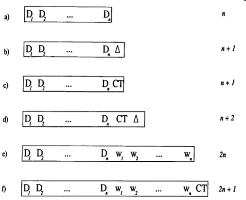
Initially, a partition is a point (lower and upper limits are equal) on the line representing the feature dimension [38]. For instance, suppose that the first ex ample Cl of class C\ is given during the training phase (Fig. 3.1.a). If the value
a)
b)
c)d)
T W S i i C ( 1 ) i 1 ®2' C / 2 ) 1 55^!WS!5=!W5^ X 1 r ^ 3 - K r ^ 3 ' X 2 e = C } 3,class 1 * 1 S < 3 ) C , ( 4 )--- f
4 4 , f 4 " 4,class r I ^2 ■ ^ e) ■ e :{e, 7= ; 5 5 , f 5 > ®c , = Q )5,class 2 q ( n ) C / m ) c ^ d ) q ( 1 . 3 7 ) C 2 ( l ) C /2 .6 3 )of Cl for feature f is x \, that is e i j = X\ then the set of possible values for fea ture / will be partitioned into three partitions: < [—00, Xi\^undetermined, 0 >, < [xi, a;i], Cl, 1 >, < [xi, og], undetermined, 0 >; where the first element of the triple indicates the range of the partition, the second its class, and the third, called the representativeness value, the number of examples represented by the partition.
A partition can be extended through generalization with other neighboring points in the same feature dimension. The CFP algorithm pays attention to the disjointness of the partitions to avoid over-generalization. In order to generalize a partition in feature / to cover a point, the distance between them must be less than a given generalization limit (D j). Otherwise, the new example is stored as another point partition in the feature dimension / . Assume that the second example 62 is close to e\ (i.e., |xi — X2I < D j) in feature / and also of the same class. In that case the CFP algorithm will generalize the partition for Xi into an extended partition < [xi,X2],C i,2 > which now represents two examples (see Fig. 3.1.b). Generalization of a range partition is illustrated in Fig. 3.1.d.
If the feature value of a training example falls in a partition with the same class, then simply the representativeness value (number representing the ex amples in the partition) is incremented by one (Fig. 3.1.c).
If the new training example falls in a partition with a different class than that of the example, the CFP algorithm specializes the existing partition by dividing it into two subpai'titions and inserting a point partition (corresponding to the new example) in between them (see Fig. 3.1.e, f). When a partition is divided into two partitions, it is important to distribute the representativeness value of the old partition to the newly formed partitions. The CFP distributes the representativeness of the old partition among the new ones in proportional to their sizes. For instance, the representativeness value of the newly formed partitions in Fig. 3.1.e will be
n = 4 X m = 4 X X5 -X4 — Xl ’ X4 - xs X4 — Xl
train(Training Set): beg in
foreach e in Training Set foreach feature /
if class of partition(/, e/) = Cdasa th e n Wf = (1 + A )w f
else Wf = (1 — A )w /
update-feature-parti tioning(/ , e /) end
Figure 3.2. Training algorithm of the CFP
In terms of production rules, the partitioning in Fig. 3.1.f can be represented as: if e j > X i and e/ < X5 th e n ^claaa ~ C \ if e j = X 5 th e n ^claaa ~ C \ i f 6 f > X 5 and C f < X 4 th e n ^claaa ~ C \
The CFP algorithm pays attention to the disjointness of the partitions. However, partitions may have common boundaries. In this case the repre sentativeness values of the partitions are used to determine class value. For example, in Fig. 3.1.f at e/ = X5, three classes Ci, C2 and Cz are possible,
but since the total representativeness of the class C\ is 4 and that of the other classes is 1, the prediction for the feature f \s C\.
The training process in CFP algorithm has two steps: learning of feature weights and feature partitions (Fig. 3.2). For each training example, the pre diction of each feature is compared with the actual class of the example. If the prediction of a feature is correct, then the weight of that feature is incre mented by A (global feature weight adjustment rate) percent; otherwise, it is decremented by the same amount.
prediction(e):
begin
VOtCc = 0
foreach feature /
c = class of partition(/, e/)
votcc = vottc A
return class c with highest votCc· end
Figure 3.3. The Prediction process of CFP
The prediction in the CFP is based on a vote taken among the predictions made by each feature separately (Fig. 3.3). For a given instance e, the predic tion based on a feature / is determined by the value of e/. If e/ falls properly within a partition with a known class then the prediction is the class of that partition. If 6/ falls in a point partition then among all the partitions at this point the one with the highest representativeness value is chosen. If e/ falls in a partition with no known class value, then no prediction for that feature is made. The effect of the prediction of a feature in the voting is proportional with the weight of that feature. All feature weights are initialized to one before the training process begins. The predicted class of a given instance is the one which receives the highest amount of votes among all feature predictions.
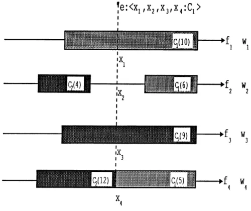
Fig. 3.4 shows an example of classification process of the CFP on a domain with four features and two classes. Assume that the test example e has a class value Cl and features values are xi, X2, X3, and X4 respectively. The prediction
of the first feature is Ci. The second feature predicts undetermined as a class value. The prediction of the third and fourth features are C2· The fourth
feature value X4 of e falls into two partitions. In this case the representativeness
values are used to determine the class value (e.g., C2 partition has greater
representativeness value than Ci partition, so that prediction of the fourth feature is C2)· Final prediction of the CFP depends on the values of the
feature weights (r/;,’s). If wi > (103 + W4) then CFP will classify e as a member
of Cl class which is a correct prediction. Otherwise, CFP predicts the class of the e as C2, which would be a wrong prediction.
The second step in the training process is to update the partitioning of each feature using the given training example (Fig. 3.5). If the feature value
|e:<Xi,X2,X3,X 4:Ci>
I f s | iii III lllllllllllil i l i H 1’"'--- III
i i iiiiliji i i I ·
Figure 3.4. The Classification process of CFP
of a training example falls in a partition with the same class, then simply its representativeness value is incremented. If the new feature value falls in a partition with a different class than that of the example and this partition is a point partition, then a new point partition (corresponding to the new feature value) is inserted next to the old one. Otherwise, if the class of the partition is not undetermined, then the CFP algorithm specializes the existing partition by dividing it into two subpartitions and inserting a point partition (corresponding to the new feature value) in between them. On the other hand, if the example falls in an undetermined partition, the CFP algorithm tries to generalize the nearest partition of the same class with the new point. If there exist a partition with the same class in D / distance, then it is generalized to cover the new feature value. Otherwise, a new point partition that corresponds to the new feature value is inserted.
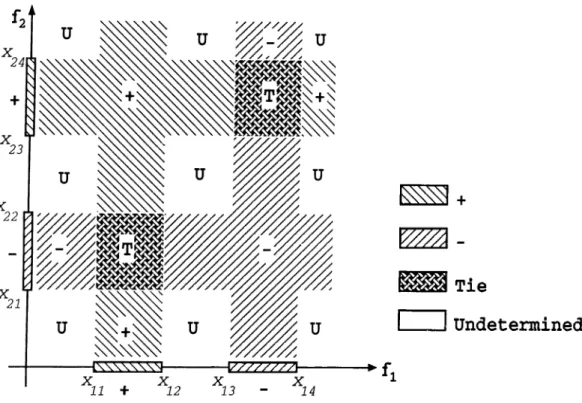
In order to illustrate the form of the resulting concept descriptions learned by the CFP algorithm, consider a domain with two features / i and / 2. Assume that during the training phase, positive (+) instances with /j values in [arn, X12] and /2 values in [3:23, 3:24], and negative (—) instances with /1 values in [3:13, 3:14] and /2 values in [3:21,^ 22] are given. The resulting concept description is shown
update-feat ure-partitioning(/, ey): beg in
if class of partition(/, ey) = edasa
increment representativeness value of partition(/, ey) else {different class}
if partition(/, ey) is a point partition insert-new-partition(/, ey)
else {partition(/, ey) is a range partition}
if class of partition(/, ey) is not undetermined subdivide-partition(partition(/, ey), ey) else (try to generalize}
if the nearest partition to left or right in D f distance has the class edass
genera,\ize{partition,e y)
else {there is no partition in D j distance with the same class as e}
insert-new-partition(/, ey) end
Figure 3.5. Updating a feature partition in Fig. 3.6.
For test instances which fall into the region [—oo, Xn][a:23, X24], for example,
feature /1 has no prediction, while feature /2 predicts as class (-|-). Therefore, any instance falling in this region will be classified as (-|-). On the other hand, for instances falling into the region [—00, 00, X2i]> for example, the CFP
algorithm does not commit itself to any prediction.
If both features have equal weight (wi = IV2) then, the description of the
concept corresponding to the class -|- shown in Fig. 3.6 can be written in 3-DNF as:
class d-:
(aJii < /1 & /1 < x\2 & /2 < 2:21) or
(a:ii < /1 & /1 < x\2 & /2 > 2:22) or
{x23 < /2 & /2 < X24 & /1 < a^is) or
{X2Z < /2 & /2 < X24 & /1 > Xu)
Tie
Undetermined
EZZZZZZZl·
X X
13 - 14
Figure 3.6. An example concept description in a domain with two features
class +:
[(a^ii < fi < xn) & (/2 < X21 or X22 < /2)] or [{.X23 < /2 < X24) ^ ifi < a:i3 or < /1 ) ]
Similarly, the description for the negative examples can be written as:
class — :
[(a:i3 < / 1 < 3:14) & (/2 < X23 or 0:24 < /2)] or [(3^21 < /2 < X22) & i f i < x n or X12 < /1)]
The CFP does not assign any classification to an instance if it could not determine the appropriate class value for that instance. This may result from having seen no instances for a given set of values or having a tie between two or more possible contradicting classifications. In case of different weight values for the features, the ties are broken in favor of the class predicted by the features with the highest weights during the voting process (with equal feature weights, it corresponds to the majority voting scheme of feature predictions).