i
IMPEDANCE BASED MODELING OF BATTERY
PARAMETERS AND BEHAVIOR
A THESIS SUBMITTED TO
THE GRADUATE SCHOOL OF ENGINEERING AND SCIENCE OF BILKENT UNIVERSITY
IN PARTIAL FULFILLMENT OF THE REQUIREMENTS FOR THE DEGREE OF MASTER OF SCIENCE IN CHEMISTRY
By
Elif Özdemir
July 2017
ii
IMPEDANCE BASED MODELING OF BATTERY PARAMETERS AND BEHAVIOR
By Elif Özdemir July 2017
We certify that we have read this thesis and that in our opinion it is fully adequate, in scope and in quality, as a thesis for the degree of Master of Science.
Burak Ülgüt (Advisor)
Şefik Süzer
Damla Eroğlu Pala
Approved for the Graduate School of Engineering and Science:
Ezhan Karaşan
iii
ABSTRACT
IMPEDANCE BASED MODELING OF BATTERY
PARAMETERS AND BEHAVIOR
Elif Özdemir M.Sc. in Chemistry Advisor: Burak Ülgüt
July 2017
Modeling battery performance under arbitrary load has gained importance in recent years with the increasing demand on batteries in various fields from automotive industry to consumer electronic devices. Due to numerous application areas of electrochemical energy storage (EES) systems, researchers have tried to predict the battery performance and the voltage using extensive calculations. Unfortunately, in order to achieve high levels of accuracy, the model has to be algebraically and computationally complex. Models with decreased computational and algebraic complexity suffer from loss of accuracy.
In this thesis, we offer a new modeling approach to predict the voltage responses of batteries and supercapacitors which is both algebraically straightforward and yielding more accurate results. Our approach is valid using any discharge profile including published by regulatory bodies such as Environmental Protection Agency (EPA).
iv
Our method is based on Electrochemical Impedance Spectroscopy (EIS) measurements done on the system to be predicted and slow DC discharge. EIS data is used directly to predict the fast moving portion of the voltage response to the profiles. The EIS data is used as is, namely, in frequency domain without any modeling. The slow DC discharge data provides DC response and is added in through a straightforward lookup table. This widely applicable approach can predict the voltage with less than 1% error, without any adjustable parameters to a large variety of discharge profiles.
Keywords: Electrochemical Impedance Spectroscopy, Battery Modeling, Battery, Supercapacitor
v
ÖZET
BATARYA KARAKTERİSTİK ÖZELLİK VE
DAVRANIŞLARININ EMPEDANS TEMEL ALINARAK
MODELLENMESİ
Elif Özdemir Kimya, Yüksek Lisans Tez Danışmanı: Burak Ülgüt
Temmuz 2017
Otomotiv endüstrisinden tüketici elektroniğine kadar çeşitli alanlarda pillere olan talebin artması ile pil performansının herhangi bir yük altında modellenmesi son yıllarda önem kazandı. Elektrokimyasal enerji depolama (EES) sistemlerinin çok sayıda uygulama alanı nedeniyle, araştırmacılar kapsamlı hesaplamaları kullanarak pil performansını ve voltajını tahmin etmeye çalışıyorlar. Ne yazık ki, yüksek düzeyde doğruluk elde etmek için modelin cebirsel ve hesaplama açısından karmaşık olması gerekir. Azalan hesaplama ve cebirsel karmaşıklığı olan modellerde doğruluk kaybı yaşanır.
Bu tezde hem piller hem de süperkapasitlerdeki gerilim tepkilerini öngörmek için cebirsel açıdan basit ve daha doğru sonuçlar veren yeni bir modelleme yaklaşımı
vi
sunuyoruz. Yaklaşımımız, Çevre Koruma Ajansı (EPA) gibi düzenleyici kurumlar tarafından yayınlanan herhangi bir deşarj profili için geçerlidir.
Yöntemimiz, tahmin edilecek sistem üzerinde yapılan Elektrokimyasal Empedans Spektroskopisi (EIS) ölçümlerine ve yavaş DC deşarjına dayanmaktadır. EIS verileri, profillere voltaj tepkisinin hızlı hareket eden bölümünü tahmin etmek için doğrudan kullanılır. EIS verileri olduğu gibi, yani herhangi bir modelleme olmaksızın frekans alanında kullanılır. Yavaş DC deşarj verileri DC yanıtı sağlar ve basit bir arama tablosu aracılığıyla eklenir. Bu yaygın uygulanabilir yaklaşım, büyük bir aralıktaki deşarj profilleri için herhangi bir ayarlanabilir parametre olmaksızın,% 1'den daha az hatayla gerilimi öngörebilir.
Anahtar Sözcükler: Elektrokimyasal Empedans Spektrokopisi, Batarya Modellemesi, Batarya, Süperkapasit
vii
Acknowledgement
During this two-year extensive working, I have had many precious people that support me and assist me whenever I need a help and support. Even if thanking them for all they’ve done for me is not enough to reciprocate their favors, supports and help, I owe them a depth of gratitude.
First and foremost, I would like to express my deepest gratitude to my supervisor Asst. Prof. Burak Ülgüt for his excellent guidance, immense knowledge, patience and enthusiasm. Whenever I feel lost, he instilled hope into me to pursue my way. I have learnt a lot from him. He was a great source of inspiration and I could not have imagined having a better supervisor.
My sincere thanks are also to the esteemed Prof. Şefik Süzer and Prof. Hitay Özbay for their support and assistance.
Special thanks also to my groupmate Can Berk Uzundal for his help, support and friendship. Moreover, to my besty Mürşide Rabia Erdoğan; I truly appreciate that I have her friendship. I will miss our coffee break and cinema ritual.
I would like to thank my friends Elif Pınar Alsaç, Elif Perşembe, Nüveyre Canpolat, Merve Balcı, Menekşe Liman, Tuluhan Olcayto Çolak and Muammer Yusuf Yaman for making the days here very fun and memorable. Also, I thank my other colleagues at Bilkent University Chemistry Department, as well.
Last but not the least; I would like to thank my dear family for their encouragement and support during my entire studies. My dad and mom always stand by me for help.
viii
My dad always says “There is always another way”. I have learnt from my dad not to give up. My mom is also my friend, my elder sister and my confidante. She always brightens my way in the life by her advice. Above all she is a great mom. My elder brother is always my role model. He always leads the way to show me how to handle difficulties. My little sister, she is our source of joy. Her determination sets the pace for me. I love you all. So glad I have you.
ix
Contents
1. Introduction ... 1
1.1. Energy Storage Systems ... 1
1.2. Batteries ... 3
1.3. Supercapacitors ... 6
1.4. Impedance ... 8
1.4.1. Electrochemical Impedance Spectroscopy and Its Applications ... 13
1.4.2. Time domain, Frequency domain and Fourier Transform ... 17
1.5. Battery Modeling ... 20
1.5.1. DC ... 22
1.5.2. AC ... 22
1.6. Scope of Current Work ... 24
2. Experimental ... 27
2.1. Experimental Part ... 28
x
2.1.2. Preferred profiles... 29
2.1.3. Procedures of the measurements ... 30
2.1.4. Error analysis ... 35
2.2. Numerical Part ... 37
2.2.1. Curve fitting using various functions and background subtraction... 38
2.2.2. Background subtraction by using piecewise linear approximation ... 40
2.2.3. Applying Singular Value Decomposition ... 42
2.2.4. Full Cycle ... 43
3. Initial Development of the Approach Using NiCd Batteries as a Testbed ... 47
3.1.FUDS profile measurement with different capacity (Imax) values ... 48
3.2. Measurement with FUDS profiles in greater lengths ... 49
3.3.FUDS profile measurement with different sampling time ... 51
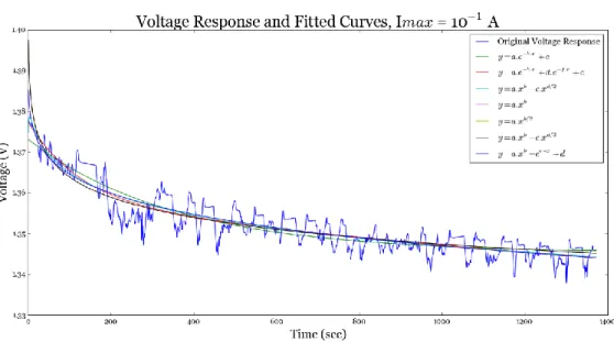
3.4. Curve fitting using various functions and background subtraction ... 53
3.5. Open Circuit Potential measurements for background subtractions of the curves …………...55
3.6. Background subtraction by using piecewise linear approximation (scipy.signal.detrend function) ... 57
3.7. Plotting voltage and current in frequency domain for background subtraction with scipy.signal.detrend function ... 60
3.8. Effect of segment length in scipy.signal.detrend function upon background subtraction ... 61
xi
3.9. Arranging segment length in scipy.signal.detrend function based on values in
data instead of using equal segments for background subtraction ... 63
3.10. Applying Singular Value Decomposition to voltage values of FUDS and OCP ... 65
3.11.Impedance measurement via Gamry instrument ... 66
3.12.Full Cycle ... 68
3.12.1. Returning time domain ... 69
3.12.2. Difference of the measured and calculated voltage in time domain ... 71
3.12.2.1. Shifting the calculated voltage data ... 72
3.12.3. Comparing measured and calculated voltage in frequency domain ... 74
3.13. Discharging the battery with constant current mode ... 76
3.14.Leaving the batteries resting for reaching their own equilibrium ... 78
3.15.FUDS profile measurement with a battery having state of charge as 1.16V . 79 4. Further Development of the Model Using Batteries of Different Chemistries and Supercapacitors with Minimal Self-Discharge ... 81
4.1. Modeling Methodology ... 83
4.2. Results and Discussions ... 84
4.2.1. Details of the energy storage chemistry/mechanism ... 88
4.2.2. Discharge profile ... 89
4.2.3. Non-linearity ... 89
4.2.4. Variance of EIS characteristics with respect to SOC ... 91
xii
4.3. Conclusions ... 94
5. Error Analysis ... 95
5.1. Error Analysis ... 96
5.2. Results & Discussion ... 98
5.3. Conclusions and outlook ... 102
6. Future Work ... 103 7. Conclusion ... 107 8. Bibliography ... 109 9. Appendix ... 116 9.1. Code ... 116 9.1.1. Full Cycle ... 116
9.1.2. Curve fitting using various functions and background subtractions ... 123
9.1.3. Background subtraction by using piecewise linear approximation ... 125
xiii
List of Figures
Fig. 1. 1: Conventional way of battery and electrodes nomenclature ... 4
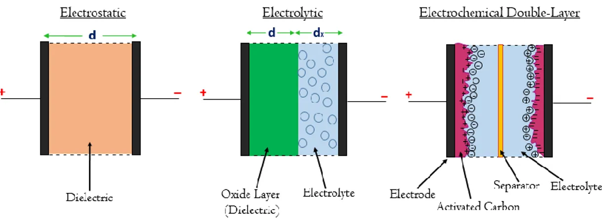
Fig. 1. 2: Schematic representation of electrostatic capacitor, electrolytic capacitor and electrochemical double-layer capacitor... 7
Fig. 1. 3: Representation of direction of current flow in a circuit with DC supply and AC supply. R corresponds to a resistor. ... 9
Fig. 1. 4: Voltage response of resistance against DC and voltage response of resistance against most common type of AC which is sine wave ... 10
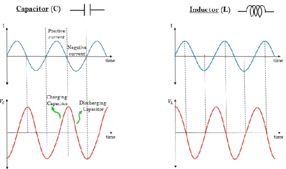
Fig. 1. 5: Current vs Time and Voltage vs Time graphs of both capacitor and inductor ... 11
xiv
Fig. 1. 6: Representations of Impedance as Nyquist and Bode Plots (These data belongs to a NiMH battery)... 12
Fig. 1. 7: Electrified Interface and its equivalent circuit model, namely, Randles Circuit. RS: Uncompensated Solution Resistance, Rct: Charge-transfer resistance, Cdl: Double layer capacitor, ZW: Warburg impedance, OHP: outer Helmholtz plane, and IHP: inner Helmholtz plane). ... 14
Fig. 1. 8: Two different sine waves [sin(2π4t)and sin(2π12t),respectively] in time domain and their correspondence in frequency domain ... 18
Fig. 1. 9: Sum of the previous signals in both time and frequency domain ... 19
Fig. 1. 10: Steps of the methodology ... 26
Fig. 2. 1: Speed vs Test Time of HDUDDS and Highway-FET driving Schedules.. 30
Fig. 2. 2: The procedure used to estimate currents based on drive schedules of the EPA ... 31
Fig. 2. 3: The current profiles used in this work as an example, 350 mA amplitude profiles are shown that were used for the 350F... 33
xv
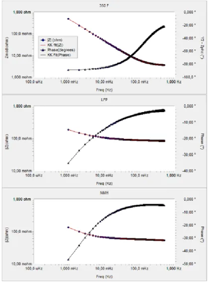
Fig. 2. 4: The Impedance Spectra and the Kramers-Kronig transforms for the three systems measured in the relevant frequency region 350F (top), LFP (middle), NiMH (bottom) ... 34
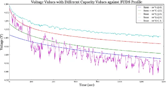
Fig. 3. 1: Voltage response of the NiCd battery to applied FUDS profile at different capacity values ... 49
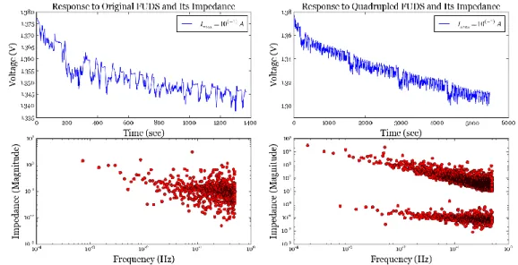
Fig. 3. 2: Voltage responses of the NiCd battery to applied FUDS profile (top left) and quadrupled FUDS profile (top right), and Magnitude of their impedance (bottom row - red). ... 50
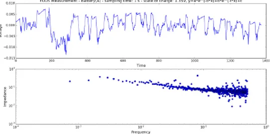
Fig. 3. 3: Voltage response of the battery (top) to FUDS profile with 0.01 s sampling time and 10-1 A maximum capacity (Imax), and Magnitude of its impedance (bottom). ... 51
Fig. 3. 4: Voltage response of the battery to FUDS profile with 1 s sampling time and 10-1 A maximum capacity (Imax), and Magnitude of its impedance. ... 52
Fig. 3. 5: Voltage response of the battery (top) to FUDS profile with 10 s sampling time and 10-1 A maximum capacity (Imax), and Magnitude of its impedance (bottom). ... 52
Fig. 3. 6: Various analytical functions that are fitted to the voltage response of the NiCd battery ... 53
xvi
Fig. 3. 7: The residuals after each of those analytical functions is subtracted from the voltage response of the NiCd battery ... 54
Fig. 3. 8: Open Circuit Potential (OCP) curves of the NiCd battery at 0.01 s (top), 1 s (middle) and 10 s (bottom) sampling time. ... 55 Fig. 3. 9: The residuals after each OCP curves are subtracted from the voltage response of NiCd battery to FUDS profile. Top: 0.01 s Middle: 1 s Bottom: 10 s sampling time ... 56
Fig. 3. 10: Magnitudes of the impedance of those residuals obtaining from subtraction of OCP from the voltage response of the NiCd battery. Top: 0.01 s, Middle: 1 s, and Bottom: 10 s sampling time ... 56
Fig. 3. 11: The residual voltage values after applying scipy.signal.detrend function to the voltage response of the NiCd battery to FUDS profile at 0.01 s (top), 1 s (middle) and 10 s (bottom) sampling time. The preferred segment length for the function is 343. The state-of-charge of the battery is 1.35V. ... 58
Fig. 3. 12: The residual voltage values after applying scipy.signal.detrend function to the voltage response of the NiCd battery to FUDS profile at 0.01 s (top), 1 s (middle) and 10 s (bottom) sampling time. The preferred segment length for the function is 343. The state-of-charge of the battery is 1.25V. ... 58
xvii
Fig. 3. 13: Magnitudes of the impedance belonging to those residual voltage values that scipy.signal.detrend function has been previously applied. Top: 0.01 s, Middle: 1 s, and Bottom: 10 s sampling time. The state-of-charge of the NiCd battery is 1.35 V. ... 59
Fig. 3. 14: Magnitudes of the impedance belonging to those residual voltage values that scipy.signal.detrend function has been previously applied. Top: 0.01 s, Middle: 1 s, and Bottom: 10 s sampling time. The state-of-charge of the NiCd battery is 1.25 V. ... 59
Fig. 3. 15: Left Column: Current data in frequency domain at 0.01 s (top), 1 s (middle), and 10 s (bottom) sampling time. Right Column: The scipy.signal.detrend function applied voltage values in frequency domain at 0.01 s (top), 1 s (middle), and 10 s (bottom) sampling time. The state-of-charge of the battery is 1.35 V. ... 61
Fig. 3. 16: The residual voltage values after applying scipy.signal.detrend function to the voltage response of the NiCd battery to FUDS profile at 0.01 s (top), 1 s (middle) and 10 s (bottom) sampling time. The preferred segment length for the function is 686. The state-of-charge of the battery is 1.35V. ... 62
Fig. 3. 17: The residual voltage values after applying scipy.signal.detrend function to the voltage response of the NiCd battery to FUDS profile at 0.01 s (top), 1 s (middle) and 10 s (bottom) sampling time. The preferred segment length for the function is 686. The state-of-charge of the battery is 1.25V. ... 62
xviii
Fig. 3. 18: Magnitudes of the impedance belonging to those residual voltage values that scipy.signal.detrend function has been previously applied. Top: 0.01 s, Middle: 1 s, and Bottom: 10 s sampling time. The state-of-charge of the NiCd battery is 1.35 V in the left column and it is 1.25 V in the right column. ... 63
Fig. 3. 19: The residual voltage values after applying scipy.signal.detrend function to the voltage response of the NiCd battery to FUDS profile at 0.01 s (top), 1 s (middle) and 10 s (bottom) sampling time. The determined segments for the function are (100, 300, 600, and 1200). The left column data has 1.35V state-of-charge while the right one has 1.25V state-of-charge. ... 64
Fig. 3. 20: Magnitudes of the impedance belonging to those residual voltage values that scipy.signal.detrend function has been previously applied. Top: 0.01 s, Middle: 1 s, and Bottom: 10 s sampling time. The state-of-charge of the NiCd battery is 1.35 V in the left column and it is 1.25 V in the right column. ... 64
Fig. 3. 21: Top: Singular Value Decomposition analysis of the voltage responses to FUDS and OCPs at 0.01 s, 1 s, and 10 s sampling time. Bottom: Eigenvectors of the matrix composed of voltage values of FUDS and OCPs. The state-of-charge of the NiCd battery is 1.35V. ... 65
Fig. 3. 22: The Nyquist and Bode plots of the NiCd battery at 1 s sampling time. The state-of-charge of the battery is 1.35V. ... 66
xix
Fig. 3. 23: Magnitudes of both the measured impedance (top) and calculated impedance (bottom) at 1 s sampling time. The state-of-charge of the battery is 1.35V. ... 67
Fig. 3. 24: The Nyquist and Bode plots of the NiCd battery at 1 s sampling time. The state-of-charge of the battery is 1.25V. ... 67 Fig. 3. 25: Magnitudes of both the measured impedance (top) and calculated impedance (bottom) at 1 s sampling time. The state-of-charge of the battery is 1.25V. ... 68
Fig. 3. 26: Top: The measured voltage response to the applied FUDS profile. Middle: The calculated voltage response obtained via the Full Cycle method. Bottom: The current data. All measurements done here have 0.01 s sampling time. Left column: The state-of-charge of the battery is 1.35V. Right column: The state-of-charge of the battery is 1.25V. ... 69
Fig. 3. 27: Top: The measured voltage response to the applied FUDS profile. Middle: The calculated voltage response obtained via the Full Cycle method. Bottom: The current data. All measurements done here have 1 s sampling time. Left column: The state-of-charge of the battery is 1.35V. Right column: The state-of-charge of the battery is 1.25V. ... 70
Fig. 3. 28: The measured voltage responses to the applied FUDS profile (left y-axis - blue) and the calculated voltage responses (right y-axis - red) at 0.01 s sampling time
xx
are shown here. In the top plot the state-of-charge of the battery is 1.35 while it is 1.25V in the bottom plot. ... 70
Fig. 3. 29: The measured voltage responses to the applied FUDS profile (left y-axis - blue) and the calculated voltage responses (right y-axis - red) at 1 s sampling time are shown here. In the top plot the state-of-charge of the battery is 1.35 while it is 1.25V in the bottom plot. ... 71 Fig. 3. 30: Residual voltage obtaining from the subtraction of the calculated voltage response from the measured ones. Left column: The sate-of-charge of the battery is 1.35V. Right column: The sate-of-charge of the battery is 1.25V. Top row: The sampling time is 0.01 s. Bottom row: The sampling time is 0.01 s ... 72
Fig. 3. 31: Voltage differences between the calculated voltage response and the measured ones (blue). The voltage difference between the calculated voltage responses, which have been shifted with +5, 10, 20, 30, 40, and 50 points delay, and the measured one (red plot). For all the state-of-charge is 1.35V. ... 73
Fig. 3. 32: Voltage differences between the calculated voltage response and the measured ones (blue). The voltage difference between the calculated voltage responses, which have been shifted with +5, 10, 20, 30, 40, and 50 points delay, and the measured one (red plot). For all the state-of-charge is 1.25V. ... 73
Fig. 3. 33: Imaginary and real part of both the calculated and measured voltage response infrequency domain. All have 0.01 s sampling time. The state-of-charge is 1.35V in the left column whereas it is 1.25V in right column. ... 74
xxi
Fig. 3. 34: Imaginary and real part of both the calculated (red) and measured (blue) voltage response infrequency domain. All have 1.0 s sampling time. The state-of-charge is 1.35V in the left column whereas it is 1.25V in right column. ... 75
Fig. 3. 35: Bode Plots of both the calculated and measured voltage responses. For all, the sampling time is 0.01 s. The state-of-charge is 1.35V in the left column whereas it is 1.25V in right column. ... 75
Fig. 3. 36: Bode Plots of both the calculated and measured voltage responses. For all, the sampling time is 1.0 s. The state-of-charge is 1.35V in the left column whereas it is 1.25V in right column. ... 76
Fig. 3. 37: Discharge curve at 0.127 mA (red) and the measured voltage response (blue) to the FUDS profile. In the left column, the state-of-charge is 1.35V while it is 1.25V in the right column. For the top row, the sampling time is 1.0 s whereas it is 10 s for the bottom row. ... 77
Fig. 3. 38: Discharge curve at 0.255 mA (red) and the measured voltage response (blue) to the FUDS profile. The sampling time is 1.0 s for the top, and 10.0 s for the bottom. The state-of-charge for both is 1.35V. ... 78
Fig. 3. 39: (Top - blue) the voltage responses of the battery to the applied FUDS profile and (bottom - red) magnitudes of their calculated impedance. The state-of-charge of
xxii
the batteries is 1.16 V here and the sampling time is 0.01 s. Left column belongs to the battery named A while right column represents the battery named B. ... 79
Fig. 3. 40: (Top - blue) the voltage responses of the battery to the applied FUDS profile and (bottom - red) magnitudes of their calculated impedance. The state-of-charge of the battery is 1.16 V here and the sampling time is 1.0 s. Left column belongs to the battery named A while right column represents the battery named B. ... 80
Fig. 4. 1: The response of LFP (in red) and the predicted value (in blue) for three profiles. Squarewave applied at 22 mA and both Highway-FET and HDUDDS applied at 220 mA. ... 85
Fig. 4. 2: The response of NiMH (in red) and the predicted value (in blue) for three profiles at 120 mA. ... 86
Fig. 4. 3: The response of 350F (in red) and the predicted value (in blue) for three values at 350 mA. ... 87
Fig. 4. 4: Selected experiments with varying amplitudes across different systems: a. Squarewave profile applied to LFP at 2.2 mA, b. Squarewave profile applied to LFP at 220 mA, c. Highway-FET applied to 350F at 350 mA, d. Highway-FET driving schedule applied to NiMH at 600 mA, e. HDUDDS applied to NiMH at 600 mA. . 90
Fig. 4. 5: The profiles repeated for LFP at 3.12V. The current amplitudes are chosen to be the same for the 3.34V experiment ... 92
xxiii
Fig. 4. 6: The response of LFP (in red) and the predicted value (in blue) for 2.2A discharge amplitude for all profiles used in this study. The maximum errors are less than 2.1% for Squarewave, 0.7% for Highway FET, 0.5% for HDUDDS. ... 93
Fig. 5. 1: The calculated results (top) and the fractional error (bottom) of the modeling approach shown. The fractional errors show non-random structure, especially in the Squarewave signal. The columns show the three energy storage systems(350F, the NiMH and the the LiFePO4, where the rows show three different discharge profiles, squarewave, HDUDDS from EPA and Highway FET from EPA. ... 97
Fig. 5. 2: The results of the numerical test showing that the errors are not improving with improved sampling and that the error magnitude is too small to account for the observed errors. ... 98
Fig. 5. 3: Experimental verification that changing the sampling rate does not affect the magnitude, nor the structure of the observed errors. ... 99
Fig. 5. 4: The observed errors at different current amplitudes. At higher amplitudes, the errors go higher since the nonlinearities get worse with increasing amplitudes 100
Fig. 5. 5: The cell voltage vs. amount of discharge map for the same 350F supercapacitor measured at different discharge rates. Lower currents result in higher apparent capacitance. ... 101
xxiv
Fig. 5. 6: The effect of the quality of DC map is shown. The current values shown as column headings indicate the current that was used to collect the DC map data. ... 102
Fig. 6. 1: Characteristic Curve of Current vs Voltage showing its pseudo-linearity. ... 104
xxv
List of Table
xxvi
List of Abbreviations
350F: Supercapacitor (having 350 F capacitance) A.C.: Alternating Current
CAFE: Corporate Average Fuel Economy Cdl: Double layer capacitor
D.C.: Direct Current
EDLC: Electrical Double Layer Capacitor EIS: Electrochemical Impedance Spectroscopy EPA: Environmental Protection Agency ESS: Energy Storage System
FFT: Fast Fourier Transform
FUDS: Federal Urban Driving Schedule
xxvii
Highway-FET: Highway Fuel Economy Test iFFT: inverse Fast Fourier Transform
IHP: Inner Helmholtz Plane KK: Kramers-Kronig
LFP: Lithium Iron Phosphate (LiFePO4) NiCd: Nickel Cadmium
NiMH: Nickel Metal Hydride OCP: Open Circuit Potential OHP: Outer Helmholtz Plane Rct: Charge-transfer resistance
RS: Uncompensated Solution Resistance SEI: Solid Electrolyte Interface
SOC: State-of-charge
SVD: Singular Value Decomposition ZW: Warburg impedance
1
Chapter 1
1. Introduction
1.1. Energy Storage Systems
The main question of any energy related discussion is how the continuously rising global energy need will be fulfilled. It is a clear fact that in the 21st century the energy demand is much more increased with new improvements in technology [1]. From industry to households, large amount of power is used in almost every point of daily life for extended periods of time. Since the industrial revolution, the highest portion of the pie chart that indicates the distribution of the energy supply by different energy sources belongs to fossil fuels. The major fossil fuels are petroleum, coal, and natural gas. According to Key World Energy Statistics published by the International Energy Agency (an autonomous body within the OECD) in 2016, fossil fuels are responsible for supplying about 81 % of the world’s energy demand [2]. Certainly, the benefits of fossil fuels like being easy-to-find, efficient, easier-to-transport, and easy-set-up are
2
why they have been dominant sources for energy supply. However, the drawbacks such as environmental degradation (i.e. global warming due to released carbon dioxide resulting from the burning of fossil fuels), finite energy sources, and a threat to public health due to pollution are the main reasons why new energy sources are sought after today for meeting world’s energy demand. Besides, its fluctuating cost as a consequence of either physical conditions or political reasons in the world hinders that countries all over the world to evenly access it. This is another important reason that boosts the search of new energy sources.
As alternatives to fossil fuels, renewable energy sources such as sunlight, wind and hydro power has been indicated since they are only as finite as the sun and they mitigate carbon emissions. Nonetheless, they possess their own shortcomings. Their energy production and efficiency are controlled by external, natural and unpredictable factors [3]. Specifically, climate occurrences such as slow wind and abundant rain cause the energy production to decrease. Since renewable energy sources are not available in all locations in the world and their energy output is generally lower than comparable sized fossil fuel installations, energy generated by renewable sources tends to be stored for later use (i.e. when energy sources are in less productive time). This is where Energy Storage Systems (ESS), along with Energy Conversion Systems (ECS) are of utmost importance. Energy storage means storing produced energy to use when needed whereas energy conversion is the process of converting the energy produced from one form to another. Since energy storage systems are limited and variable in terms of their reliability, stability and reproducibility, converting the form of energy that is produced into a form that is storable with greater efficiency and lower losses is desirable.
3
ESS are classified according to form of energy that is stored. Some examples are mechanical, electrochemical, chemical, and electrical [4]. The ESS that are related to the present work are electrical and electrochemical energy storage systems. Basically, in the latter one electrochemical processes and interfaces such as redox reactions or electrochemical double layer are used in order to store energy whereas in the former one energy storage is done electrically without a chemical reaction. Batteries are one of the members of electrochemical energy storage systems while an example of electrical energy storage is supercapacitors [4].
1.2. Batteries
Battery is the main electrochemical energy storage system that is a series or parallel connection of electrochemical cells containing a positive and a negative electrode separated by an electrolyte. It can store electrical energy in the form of chemical energy during charge and transform that chemical energy back into electricity during discharge. Battery electrodes comprise of an active material and a current collector. Designation of battery electrodes can often cause confusion. In conventional way of battery design, the negative electrode is named as anode and the positive electrode is called cathode. Considering the electrochemical reactions, of course, these nomenclatures are only valid for discharge process. Fig. 1.1 indicates the traditional way of battery and electrodes nomenclature during discharge (supplying load) and charge (connected to a power supply) [5].
4
Fig. 1. 1: Conventional way of battery and electrodes nomenclature.
During discharge, oxidation which is an anodic process takes place at the negative electrode while reduction which is a cathodic process occurring at the positive electrode. During charge the electrochemical reactions are reversed: reduction occurs at the negative electrode and oxidation at the positive electrode. Thus, it is clearer and more accurate to use negative and positive electrode terms instead of naming electrodes as the anode and cathode.
The active layer of the battery electrode takes the main part in the reactions. The active layer is coated on the current collector and oxidized or reduced during the discharge and charge processes. Since the reactions for both sides of the battery electrodes occur at the interface of the electrode and the electrolyte, high surface areas are of great benefit. Therefore, porous materials are used as active ingredients as well as conductive matrices. These porous materials have to be connected to the external circuit through a wire. This connection is generally achieved using a current collector. Current collector is generally a metal that carries current efficiently in and out of the
5
electrode. Another function of the current collector is to serve as the mechanical support for the active material mixture.
Batteries can be classified as primary and secondary batteries. This classification is based on the ability of the battery to be recharged. Primary batteries are non-rechargeable batteries. These batteries work in only one direction, which is discharge. They can be used once until they totally discharge. An example of the primary batteries is commonly used alkaline batteries (Zinc/Manganese dioxide). In the alkaline battery, the negative electrode is Zn and the positive electrode is MnO2 and the electrolyte of the cell is potassium hydroxide (KOH). The reactions taking place in the cell:
𝑍𝑛(𝑠)+ 2𝑂𝐻(𝑎𝑞)− → 𝑍𝑛𝑂(𝑠)+ 𝐻2𝑂(𝑙)+ 2𝑒−
2𝑀𝑛𝑂2(𝑠)+ 𝐻2𝑂(𝑙)+ 2𝑒− → 𝑀𝑛2𝑂3(𝑠)+ 2𝑂𝐻(𝑎𝑞)−
Applying current in reverse direction, namely, trying to charge the battery can result in several problems in the alkaline battery such as irrecoverable changes in the reactants, gas formation in the electrolyte and damaging the separator. When the alkaline battery discharges, Zn is dissolved, however, the current in reverse direction cannot deposite Zn back onto the negative electrode evenly. Besides, electrolyzing the electrolyte, gas formation, which can damage the separator and the whole process, can be observed. Thus, these problems cause the reactions not to be reversible, and Zn/MnO2 cell is considered to be a primary cell, namely a non-rechargeable cell.
On the other hand, secondary batteries are called rechargeable batteries and they can be utilized multiple times through external charging even if they get discharged. Lithium-ion and Nickel-Metal Hydride batteries are two examples of the secondary batteries. In Li-ion batteries, the negative electrode is a graphitic carbon and its current
6
collector is aluminum while the positive electrode is a Li-intercalation compound (i.e. LiCoO2) and its current collector is copper [6]. The chemical reactions that occur at the electrodes during charge and discharge are shown below:
𝑥𝐿𝑖++ 𝑥𝑒−+ 6𝐶 ↔ 𝐿𝑖
𝑥𝐶6 (𝑎𝑡 𝑡ℎ𝑒 𝑛𝑒𝑔𝑎𝑡𝑖𝑣𝑒 𝑒𝑙𝑒𝑐𝑡𝑟𝑜𝑑𝑒) 𝐿𝑖𝐶𝑜𝑂2 ↔ 𝐿𝑖1−𝑥𝐶𝑜𝑂2+ 𝑥𝐿𝑖++ 𝑥𝑒− (𝑎𝑡 𝑡ℎ𝑒 𝑝𝑜𝑠𝑖𝑡𝑖𝑣𝑒 𝑒𝑙𝑒𝑐𝑡𝑟𝑜𝑑𝑒)
Here, the products of the reactions are deposited back onto electrodes, and the original reagents are obtained during the charging process. Thus, the reactions are reversible and the Li-ion batteries are considered to be secondary batteries.
1.3. Supercapacitors
Supercapacitors are an example of electrical energy storage systems. Supercapacitors are electrical storage devices that can store and release large amount of electrical charge quickly. They are the latest generation capacitors which build upon electrostatic and electrolytic capacitors. Capacitors can be categorized based on the mechanisms used to store electrical charge [7]. First generation capacitors, which are electrostatic capacitors, comprise two parallel metal electrodes and a dielectric that separates electrodes as in Fig. 1.2.
7
Fig. 1. 2: Schematic representation of electrostatic capacitor, electrolytic capacitor and electrochemical double-layer capacitor.
The dielectric is a non-conducting material interpolated between the parallel metal electrodes and boosts the overall capacitance, namely the ability to store electric charge [7]. The electrolytic capacitors have similar structure except possessing a conducting electrolyte between the electrodes (see Fig. 1.2) and very thin oxide layer coated on the electrodes acts as a dielectric and enables to have a higher capacitance per unit volume [7].
Supercapacitors or electrochemical double-layer capacitors have capacitances that are much higher compared to conventional capacitors (electrostatic and electrolytic capacitors) and hold out much higher power density than batteries [8]. As a construction they consist of parallel electrodes, electrolyte and a separator as in Fig. 1.2. The electrodes have activated carbon coated on them. This porous layer offers the electrodes to get a higher surface area that enables them to store much more electric charge. An ion-permeable membrane separates the two electrodes and makes ionic charge transfer possible. One more advantage of the membrane is to prevent electrical contact between the two electrodes from occurring. Then, all system is soaked in an electrolyte that might be of organic, aqueous or solid state type in accordance with
8
power required in applications [9]. During charging, positive charges are collected on the surface of one plate and negative charges form on the surface of the other plate. At the same time, an opposite charge emerging from ions in the electrolyte forms both side of the separator. Thus, this creates an electric double-layer inside the supercapacitor. That’s why supercapacitors are also named as electrical double-layer capacitor (EDLC) or double-layer capacitors. With the porous surface, the surface area of the plates (i.e. the effective surface area between the electrode and the electrolyte) is increased and with the double layer structure, the effective distance gets lower between the plates (i.e. charge layers) in supercapacitors. Therefore, much more electrical charge can be stored in supercapacitors than ordinary capacitors.
1.4. Impedance
Impedance (Z) can be simply described as an opposition to the flow of alternating current of an electric circuit or circuit component. Impedance exists in all circuits and in all components. In ideal cases, it follows Ohm’s Law, as well, thus, it is simply the ratio of voltage to current. However, it is a two-dimensional complex quantity composing resistance as its real part and reactance as its imaginary part. The real part represents its resistive part whereas the imaginary part represents the capacitive and inductive parts. Comprehending resistance and reactance makes better understanding of impedance concept convenient.
The idea of simple direct current electrical resistance (R) is straightforward to follow for researchers of all fields. Essentially it is the ability of a circuit component to oppose the flow of electrical current, more specifically Direct Current (DC). DC means that
9
current flows steadily in one direction, on the other hand, Alternating Current (AC) is a current which reverses its direction periodically, namely AC oscillates back and forth. Fig. 1.3 indicates the direction of current flow in a circuit when the circuit is powered by a DC supply or an AC supply.
Fig. 1. 3: Representation of direction of current flow in a circuit with DC supply and AC supply. R corresponds to a resistor.
It is assumed that DC supply provides a constant voltage over time. In the voltage versus time graph, constant voltage is observed as in Fig. 1.4. However, in actuality, charge of the supply, generally a battery, will be gradually lost and of course, voltage drop will be observed as long as the battery is used.
In AC supply since current alternates periodically, which is generally fifty or sixty times every second (50 – 60 Hz) in power outlets of houses, voltage also reverses its direction along with the current. Figure 4 also indicates voltage response of resistance against AC in the form of sine wave which is the most common type of AC.
10
Fig. 1. 4: Voltage response of resistance against DC and voltage response of resistance against most common type of AC which is sine wave
When AC goes through a resistance, waveforms of both voltage and current are in-phase, namely, both reach their maximum value at the same moment and get through zero at the same moment (see Fig. 1.4). Mathematically, phase difference equals zero (𝜑 = 0). Resistance exists prominently in resistors and it is independent of frequency.
Reactance (X) is a form of opposition to flow of current, as well. The main feature of reactance that differs from resistance is to have a particular phase angle between voltage and current responses. Reactance is present most notably in capacitors and inductors. When AC passes through a pure reactance (i.e. an ideal capacitor or inductor), the current waveform is 90 degree out of phase with the voltage waveform as it is seen in Fig. 1.5. More specifically, voltage of a capacitor (VC) lags the current by 90o and voltage of an inductor (VL) leads the current by 90o. To cite an example, when a capacitor is fully charged meaning the voltage waveform reaches its maximum value, the current waveform go through zero because no more current is required to
11
flow at this point. Similarly, during discharge, voltage value goes to zero whereas current reaches its maximum.
Fig. 1. 5: Current vs Time and Voltage vs Time graphs of both capacitor and inductor
Reactance existing in capacitors is called capacitive reactance (𝑋𝐶) and similarly, reactance that resides in inductors is designated as inductive reactance (𝑋𝐿). Both vary with frequency (𝑓). As 𝑓 increases, 𝑋𝐶 decreases and 𝑋𝐿 increases since 𝑋𝐶 and 𝑓 have an inversely proportional mathematical relationship whereas 𝑋𝐿 is directly proportional with 𝑓 as these can be seen in Eq. (1.1) and (1.2).
𝑋𝐶 = 1
2𝜋𝑓𝐶 (1.1)
𝑋𝐿 = 2𝜋𝑓𝐿 (1.2)
where 𝐶 is capacitance in Farads (F) and 𝐿 is inductance in Henrys (H).
In general, combination of these two, namely ohmic resistance and capacitive/inductive reactance, forms impedance (Z). Of course, impedance of a
12
resistor has only real part, thus, mathematically impedance equals resistance (𝑍 = 𝑅). Moreover, impedance of a capacitor or an inductor has only imaginary part and, hence, it equals capacitive or inductive reactance, respectively (𝑍 = 𝑋𝐶 𝑜𝑟 𝑍 = 𝑋𝐿).
Impedance is represented in both Cartesian form and polar form. Cartesian form as in Eq. (1.3) makes addition and subtraction of impedance convenient whereas the polar form in Eq. (1.4) clearly indicates its magnitude and phase shift and also, it is more convenient when it is needed to multiply or divide impedance.
𝑍 = 𝑅 + 𝑗 ∗ 𝑋 (1.3)
𝑍 = 𝑍0∗ exp(𝑗 ∗ 𝜙) = 𝑍0∗ (𝑐𝑜𝑠𝜙 + 𝑗 ∗ 𝑠𝑖𝑛𝜙) (1.4)
where 𝑅 is resistance, 𝑗 represents imaginary unit (√−1), 𝑋 is reactance, 𝑍0 is magnitude of 𝑍 and 𝜙 represents phase shift between voltage and current. Impedance measurement can be represented with two types of plots as it can be seen in Fig. 1.6.
Fig. 1. 6: Representations of Impedance as Nyquist and Bode Plots (These data belongs to a NiMH battery)
13
One of them is a complex plane plot which indicates the real part on the x-axis and the imaginary part on the y-axis [10]. It is called “Nyquist Plot”. It possesses a special feature that 1 cm corresponds to particular Ohm value on both x and y-axis. A disadvantage of this plot is that frequency values cannot be seen unless it is assigned on the curve. It can only be predicted that the high frequency side is the left of the plot and the low frequency side is the right of the plot. The other type is “Bode Plot” which includes two plots [10]. They are magnitude of impedance versus corresponding frequency values in logarithmic scale (𝑙𝑜𝑔𝑍0 𝑣𝑠 𝑙𝑜𝑔𝑓) and phase shift versus logarithmic frequency (𝜙 𝑣𝑠 𝑙𝑜𝑔𝑓). A disadvantage of the Bode Plot is that it is logarithmic.
1.4.1. Electrochemical Impedance Spectroscopy and Its Applications Impedance is frequency dependent and measured as a function of the frequency of the AC source. Electrochemical Impedance Spectroscopy (EIS) is a technique where impedance of an electrochemical system is measured vs. frequency. This technique studies the response of the electrochemical system to an applied electrical perturbation, namely potential or current, which is periodical small amplitude AC signal [11].
EIS provides a large amount of information although it cannot answer all questions. In batteries and supercapacitors, EIS is routinely utilized to examine the electrode kinetics and reactions taking place there [12] and to determine capacitance and resistance [10]. It has many applications including interfacial processes such as redox reactions at electrodes, adsorption and electrosorption; geometric effects such as linear, spherical, cylindrical mass transfer and determination of solution resistance;
14
and applications in power sources such as corrosion, coatings and paints, electrocatalytic reactions and sensors [10].
Examining EIS data enables resolution of the nature of the electrode kinetics and its distinctive parameters. To perform the analysis correctly, an appropriate model is required. This is done using equivalent circuit analysis which consists of simple electrical circuit elements such as resistor, capacitor and inductor in series or parallel. Fig. 1.7 indicates an electrified interface and its corresponding electrical circuit model which is well-known Randles Circuit [13]. Each component on the interface is represented by a particular electrical circuit element. More specifically, lining up of the countercations along the surface and the negatively charged electrode display capacitor like behavior, namely electrochemical double layer, thus, this behavior is expressed as Cdl in the equivalent circuit model [14].
Fig. 1. 7: Electrified Interface and its equivalent circuit model, namely, Randles Circuit. RS: Uncompensated Solution Resistance, Rct: Charge-transfer resistance, Cdl: Double layer capacitor, ZW:
15
Any charge transfer between electrode and electrolyte due to an electrochemical reaction such as electrochemical dissolution of the electrode into the electrolyte forms resistance and is represented by a resistor as Rct. Diffusion of reactant in the electrode or mass transport effect can create impedance and it is expressed as Warburg impedance, ZW. Lastly, the uncompensated solution resistance or electrolyte resistance is represented by a resistor called RS. The charge transfer resistance (Rct) and Warburg impedance (ZW) are connected in series and the capacitor (Cdl) is connected to them in parallel. The circuit is completed by connecting the electrolyte resistance (RS) in series to all of them. The simplified version of Randles circuit does not cover ZW and its Nyquist plot is always a semicircle. The ZW appears as like a straight, 45° line at the low frequency side of the Nyquist plot. The intercept of the semicircle on the real axis at the high frequency side, which is near the origin of the plot, gives the RS value whereas the other intercept at the low frequency side shows the sum of RS and Rct. Thus, the diameter of the semicircle gives the exact Rct value. Randles circuit is a simple yet fundamental example of equivalent circuit models, but different battery systems can be adapted different types of electrical circuit.
In general, the frequencies used are limited by the stability of the system in low frequency end and the response time of the electrode double layer capacitance in the high frequency end. The EIS frequency range has a broad spectrum, namely, from as low as 10 μHz for sufficient resolution of interfacial processes, up to 10 MHz or higher, sometimes needed to portray bulk response of the material of interest [15]. This gives the technique its unique ability to resolve effects that are widely varying in time-scales. As a simple example, impedance of a Li-ion battery had been measured by Osaka et.al. in the frequency range of 100 kHz to 0.1 mHz (corresponds to 10 μs to 10000 s ~3 h)
16
in order to separate and analyze each elemental processes taking place in the battery [16]. Moreover, to date, many research concerning correlation between EIS and material investigation has been published. More precisely, EIS permits the dynamics of the each basic process of the battery reactions to be delicately and separately examined and it does not distract the cell during the measurement [16]. For instance, as regards lithium-ion battery studies, the charge transfer resistance, solid electrolyte interface and the activation energies of the system such as carbonaceous materials [17] [18], silicon nanowire [19], Si-OC composite [20] for the negative electrode have been characterized by using EIS [16]. Moreover, the impedance response of an entire Li-ion battery consists of the response of the positive and negative electrodes, and the electrolyte with separator [16]. The fundamental processes that are presumed to have an impact on the impedance response are electron migrations in a conductive additive [21] and at interface of active material/current collector [22], charge transfer processes, a solid state diffusion consists of finite length Warburg [23] [24]. It is possible to distinguish the response of the two electrodes and the electrolyte with separator, at which these fundamental processes take place, from the impedance response of an entire Li-ion battery by introducing a reference electrode to the cell or using a symmetric or temperature-controlled cell [16].
On top of that, enlargement of the small impedances and shifting of the overlapping frequency domains so as to accurately examine lithium batteries with low impedance are of the view as other possible methods [16]. The resistance and interfacial capacitance values are the principle electrochemical parameters examined in EIS-based investigations [16]. In the literature, increase in the resistance of Li-ion batteries at low temperatures have been revealed since there is a strong inverse relationship
17
between the mass transfer of charged carriers and temperature [25] [26]. Hence, expanding of the impedance of Li-ion battery by decreasing temperature has been studied by Osaka et al. to differentiate between the responses of the fundamental steps in a Li-ion battery, and thus, impedance data had been acquired in the -20 and 20°C temperature range [16]. Based on the findings belonging to Osaka et al. the frequency domain of solid-electrolyte interface (SEI) impedance response had been discovered to overlap with that of the inductive segment of the external electric lead at 20°C, that’s why, it has been concluded that impedance measurements at low temperature are thought to be advantageous for determination of the SEI contribution to Li-ion battery reactions [16].
Aside from the usage of EIS to research and analyze corrosion of metals, adsorption and desorption to electrode surface, the electrochemical synthesis of materials, the catalytic reaction kinetics, the ions mobility in energy storage devices such as batteries and supercapacitors, and battery modeling [27] etc., it has gained more popularity in recent years in a wide variety of application areas such as dental application based on an observation of demineralization of human dentine by acid [28], biosensor application based on detection of tumor necrosis factor [29], and immunosensor application based on detection of HbA1c, the main diabetes marker protein [30], etc.
1.4.2. Time domain, Frequency domain and Fourier Transform Time (t) domain and frequency (f) domain analyses are terms related frequently to the investigation of signals and systems. Basically, both are alternative ways for representing signals. Time domain is an analysis of signal versus time. In a t-domain graph such as how a signal changes with respect to time, namely amplitude of the
18
signal is seen. Frequency domain is an analysis of signal over frequency. An f-domain graph indicates how much of the signal exists within each given frequency band over a range of frequencies. Also, it can give information about the phase shift of the signal. The graphs on the left in Fig. 1.8 indicates two different sine waves with particular frequencies in time domain. It gives information about their amplitude and shape of the signals. The graphs on the right in Fig. 1.8 tell how these two sine waves look like in frequency domain. It gives their position in the frequency axis which are 4 and 12 Hz, respectively, and their amplitude, as well.
Fig. 1. 8: Two different sine waves [sin(2π4t)and sin(2π12t),respectively] in time domain and their correspondence in frequency domain
19
Fig. 1.9 points out the sum of these signals in both time and frequency domain. When there are more than one wave mixing with each other, it is hard to distinguish each wave from each other in time domain graph. In fact, it is not very simple to understand what’s going on there. However, in the frequency domain graph it is easier to see that there are two waves with different frequencies. In real life signals can be much more complicated than these examples. Thus, frequency domain can provide to analyze signals conveniently.
Fig. 1. 9: Sum of the previous signals in both time and frequency domain
Time domain and frequency domain can be transformed into each other with the help of a mathematical relationship called Fourier Transform. What Fourier transform does
20
is that basically it takes t-domain signal and expresses it in terms of frequencies that form that signal by a mathematical function. It gives both amplitude and phase information about the signal. The Fourier Transform of a function 𝑔(𝑡) is in Eq. (1.5):
ℱ{𝑔(𝑡)} = 𝐺(𝑓) = ∫ 𝑔(𝑡)𝑒−2𝜋𝑗𝑓𝑡𝑑𝑡 +∞
−∞
(1.5)
It is a reversible function so that conversion from t-domain to f-domain is done by Fourier transform and the opposite conversion is made by inverse Fourier transform as in Eq. (1.6): ℱ−1{𝐺(𝑓)} = ∫ 𝐺(𝑓)𝑒2𝜋𝑗𝑓𝑡𝑑𝑓 = 𝑔(𝑡) +∞ −∞ (1.6)
1.5. Battery Modeling
Battery modeling or mathematical description of batteries has gained importance recently as battery powered applications increase. Battery modeling provides more information about the battery and estimates of its performance, runtime, capacity etc. beforehand at specific conditions of interest. Instead of trying to measure the response of the battery with respect to every discharge profile of interest, applying all desired profiles to a built model will be much easier when testing becomes too impractical. A 10-20 years life test for automotive applications is a good example of real life measurements.
In the literature, the battery models developed can be divided into two: first principle based models and equivalent circuit based models. First principle models require the
21
knowledge of numerous parameters regarding the kinetics and transport of various materials inside the system. Equivalent circuit based models, as understood from the name, use equivalent circuit modeling and then use the equivalent circuit models in time domain through a SPICE type approach [31] [32]. In this approach, the components used in the impedance fitting are converted into a time domain analog in order to model the time domain response of the system [33] [34]. Although these two groups of modeling approaches have been applied successfully in many cases, they have some drawbacks. In first principle models, since most of parameters are not exactly known, this issue turns the problem into one of fitting with numerous parameters, which ends up over-defining the problem. With the high degree of free parameters, the number of degenerate solutions increase greatly, in turn, decreasing the accuracy of the fit parameters obtained, precluding any reliable quantitative analysis. In the equivalent circuit based model, it is possible to define the circuits in a way to make sure that the number of degenerate solutions are minimized. However, these simplified circuit models (Simplified Randles and derivatives) fail to capture the full detail of the impedance spectrum [35]. There are models developed in the literature that do capture the fine detail in the impedance spectrum, however, these models have to take into account the porous structure of the electrodes and are generally based on transmission lines. These models are defined in the frequency domain and they are very complicated to get converted into the time domain.
Battery voltage is the principal response of the battery as a function of applied current profiles. The elemental parameter dictating the battery voltage response is the state-of-charge (SOC). In any battery chemistry, an electrochemical potential is present as a function of the activities of the several electroactive species. In theory, this potential
22
can be described utilizing the appropriate combination of the relevant group of Nernst Equations [36]. Electrochemical potential serves the basis for any modeling approach [37]. Nevertheless, it only reflects the thermodynamic equilibrium condition and does not capture the response of the batteries to current spikes or oscillating currents. Therefore, any fast moving current or voltage response of the battery needs to be modeled in addition to equilibrium voltage of the battery. Here, any fast moving current or voltage response of the battery is designated as AC response while equilibrium voltage of the battery is called DC response. Thus, the sum of the AC response and the DC response yields the actual real-time battery voltage.
1.5.1. DC
As previously mentioned, DC potential represents equilibrium voltage of batteries and its basis leans on electrochemical potential that emerges as a result of chemical reactions in the battery. In order to model the DC response of the battery, literature methods, along with the method developed within this thesis, uses an experimental approach. In theory, this should be approximated by a combined Nernst equation (Eq. 1.4) of all the reactions that are taking place inside the battery [36].
𝐸 = 𝐸𝑜− 𝑅𝑇
𝑛𝐹∗ 𝑙𝑛𝑄 (1.4)
where 𝑅 is gas constant, 𝑇 is temperature, 𝑛 is number of electron, 𝐹 is Faraday constant and 𝑄 is reaction quotient. Experimentally, it is obtained by forming a simple lookup table of voltage as a function of state-of-charge (SOC) and the details of the method is explained in the experimental part. This is a common method in the literature
23
[38] and the literature holds similar methods for modeling open circuit potential, as well [39].
1.5.2. AC
As stated above, AC voltage is considered to be the non-equilibrium response of batteries against any applied load. In the literature, there exists various modeling methods to simulate AC response of batteries such as electrochemical models, empirical models, equivalent electrical-circuit based models [38]. Electrochemical models intends to catch dynamic behavior of batteries on a macroscopic scale and generally they manage to give results with high accuracies [38]. These kind of models are described by using a high number of partial differential equations (PDE) that must be solved at the same time [38]. Increase in the number and order of the PDEs makes the electrochemical models more complex and can cause enormous requirements for memory and computational power [38]. Furthermore, the PDEs all require the knowledge of fundamental parameters regarding the materials and the interfaces, which are not always available.
Empirical models [40] usually adopt empirically derived equations from experimental data fittings to extrapolate correlation between several battery parameters such as the terminal voltage and SOC [38]. As an example of empirical models, some models endeavor to catch non-ideal discharge behavior utilizing moderately basic equations (i.e. Peukert’s law [41]) in which the parameters coincide with empirical data, however, in spite of the fact that simple to arrange and utilize, Peukert's law does not represent time-varying loads. [42].
24
Equivalent electrical-circuit based models provide an equivalent representation of a battery via electrical circuit models as addressed previously. These type of models have gained a ton of interest for real-time battery state estimation and power management purposes since their simplified mathematical and numerical approaches reduce the need for computationally intensive methodologies [38]. They involve a resistor-capacitor network by aiming to mimic behavioral response of batteries. Thus, they give a chance to characterize the battery response including diffusion and charge transfer processes. In the literature, the number of parallel RC networks varies depending on applied load or obtaining modeling accuracy (one-RC [43] [44], two-RC [45] [46] or more [47]). As another example, Sean Gold has offered PSPICE circuits comprising linear passive elements, voltage sources, and lookup tables to model lithium-ion batteries [48].
On the other hand, EIS based modeling approaches have been preferred, as well [49]. Although to deal with the complexity of modern automotive power nets, simulation-based design techniques are vital and appropriate models of all system components involving the battery as a fundamental part are thus mandatory, nevertheless, simulation models of energy storage devices are hard to obtain since batteries vary with time and they are strongly non-linear [49]. Therefore, the impedance-based modeling has been applied to handle these kind of difficulties. Mentioned references demonstrate that this kind of approach can regenerate the voltage profiles, as accurately as the equivalent circuit model parameters regenerate the impedance spectrum.
Simple models with one-RC network (i.e. Randles cell) clearly fail to capture all the details of EIS data. However, taking the more complex models into time domain makes
25
the algebra complicated and extend greatly the relevant computation time for the modeling.
1.6. Scope of Current Work
In this thesis, a new approach that combines the best of the two modeling approaches mentioned above is presented. Instead of modeling the impedance spectra utilizing an equivalent circuit model that is either incomplete or very complex, an approach to utilize the raw impedance data without any parametrization will be presented. Our approach makes zero assumptions and possesses no fit parameters, instead, it utilizes directly, the measured impedance spectrum to predict the response. Instead of trying to acquire battery parameters from impedance spectra in order to build a response function in the time domain, modeling is done in the frequency domain for the AC part of the response. At first, the frequency domain current profile is obtained via a Fourier transform of the desired current profile. Then, this frequency domain current profile is simply multiplied by the impedance at every frequency of interest contained by the transform. This step produces the AC voltage response of the battery. Ultimately, the voltage response of the batteries in the time domain is obtained by a simple inverse Fourier transform of the voltage profile. The whole methodology is completed by adding the DCresponse of the battery in through a simple map of SOC vs DC potential acquired experimentally.
26
Fig. 1. 10: Steps of the methodology
As indicated in the Fig. 1.10, this offered approach is computationally pretty simple and very straightforward to implement. All steps of the approach are doable analytically and do not include any approximations or assumptions.
27
Chapter 2
2. Experimental
The current chapter of the thesis is divided into two separate subunits as experimental and numerical parts. In the experimental part there is empirical information such as which type of energy storage systems (i.e. batteries, supercapacitors) and instruments have been used during the measurement, and what the preferred profiles are and also why they have been chosen. Moreover, how all the measurements have been performed is explained in detail. On the other hand, the scripts that have been utilized in order to execute the proposed modeling approach are explained in the numerical part. Besides, number crunching codes associated with the graphs which had been plotted after performing some functions to data during the initial development of the approach is explained in the numerical part, as well.
28
2.1. Experimental Part
2.1.1. Energy storage systems and instruments employed:
In the whole experimental process, batteries with different chemistries and a supercapacitor as representatives of various electrochemical energy storage systems have been employed. In the initial development of the approach, 4/5SC 1500 mAh Nickel-Cadmium (NiCd) batteries from TNL Technologies had been used. After facing some problems with the NiCd batteries that are explained in detail in chapter 3, two kinds of batteries and a supercapacitor were used, those batteries are Lithium-Iron Phosphate (LiFePO4) and Nickel-Metal Hydride (NiMH) batteries. IFR 22650 LiFePO4 battery was from EWT Battery (Shenzhen, China). The NiMH battery was 1200 mAh NiMH battery from GPI International Limited (Hong Kong). In addition, the supercapacitor was BCAP0350, a 350 F ultracapacitor from Maxwell Technologies (USA). All these samples were procured from local wholesalers. Throughout the thesis, LiFePO4 battery was denoted by LFP and the 350 F supercapacitor was designated as 350F.
During testing of the approach, measurements of impedance, DC potential vs SOC, the response to the discharge profile chosen, open circuit potential and
discharge were conducted by Gamry Interface 5000E
Potentiostat/Galvanostat/ZRA. Customs scripts had been written in-house using EXPLAIN language employed by the Gamry Framework software for the current profiles utilized in the thesis, along with impedance spectra at relevant frequency values.
29
2.1.2. Preferred profiles:
The chosen profiles in this thesis are Federal Urban Driving Schedule (FUDS), Heavy Duty Urban Dynamometer Driving Schedule (HDUDDS), Highway Fuel Economy Driving Schedule (Highway-FET) and a made-up profile named Squarewave. All driving schedules except for Squarewave are published by Environmental Protection Agency (EPA) [50]. As required by law in USA, the automobile companies need to have standards of their vehicle fleet conformed to CAFE standards [51] profile before they commence production based on these profiles. Otherwise, they are punished by extra taxes for higher CO2 emission of their vehicle fleet as leading to air pollution.
FUDS is an auto industry standard vehicle time-speed profile for urban driving that has been utilized for various years for electric vehicle performance testing and it is indistinguishable to the EPA Urban Dynamometer Driving Schedule [3]. Heavy Duty Urban Dynamometer Drive Schedule (HDUDDS) is for urban heavy duty vehicle testing and Highway Fuel Economy Test (Highway-FET) represents highway driving circumstances [52]. Moreover, Squarewave profile stands for slow conditions. In actuality, they had been arbitrarily chosen. Since the idea of this project was formulated many years ago, the well-known, common driving schedule at that time, FUDS, has been worked with in the beginning of the research. After that, the freshly published drive schedules mentioned above have been utilized. To illustrate, Fig. 2.1 indicates Highway-FET and HDUDDS profiles.
![Fig. 1.7 indicates an electrified interface and its corresponding electrical circuit model which is well-known Randles Circuit [13]](https://thumb-eu.123doks.com/thumbv2/9libnet/5794993.117944/41.892.179.819.714.1055/indicates-electrified-interface-corresponding-electrical-circuit-randles-circuit.webp)
![Fig. 1. 8: Two different sine waves [sin(2π4t)and sin(2π12t),respectively] in time domain and their correspondence in frequency domain](https://thumb-eu.123doks.com/thumbv2/9libnet/5794993.117944/45.892.247.708.487.1011/fig-different-waves-respectively-domain-correspondence-frequency-domain.webp)
![Fig. 2. 1: Speed vs Test Time of HDUDDs and Highway-FET driving schedules [50]](https://thumb-eu.123doks.com/thumbv2/9libnet/5794993.117944/57.892.210.819.145.530/fig-speed-test-time-hdudds-highway-driving-schedules.webp)