Asset pricing in a multiperiod securities market with nonnegative wealth constraints

ASSET PRICING IN A MULTIPERIOD

SECURITIES MARKET WITH

NONNEGATIVE WEALTH

CONSTRAINTS

A Ph.D Dissertation

by

YAKUP ESER ARISOY

Department of Management Bilkent University

Ankara

ASSET PRICING IN A MULTIPERIOD

SECURITIES MARKET WITH

NONNEGATIVE WEALTH

CONSTRAINTS

The Institute of Economics and Social Sciences of

Bilkent University

by

YAKUP ESER ARISOY

In Partial Fulfilment of the Requirements for the Degree of

DOCTOR OF PHILOSOPHY

in

THE DEPARTMENT OF MANAGEMENT BILKENT UNIVERSITY

ANKARA

I certify that I have read this thesis and have found that it is fully adequate, in scope and in quality, as a thesis for the degree of Doctor of Philosophy in Management.

_________________________

Assoc. Prof. Dr. Aslıhan Altay-Salih Supervisor

I certify that I have read this thesis and have found that it is fully adequate, in scope and in quality, as a thesis for the degree of Doctor of Philosophy in Management.

_________________________

Assoc. Prof. Dr. Levent Akdeniz Examining Committee Member

I certify that I have read this thesis and have found that it is fully adequate, in scope and in quality, as a thesis for the degree of Doctor of Philosophy in Management.

_________________________

Prof. Dr. Mustafa Pınar

Examining Committee Member

I certify that I have read this thesis and have found that it is fully adequate, in scope and in quality, as a thesis for the degree of Doctor of Philosophy in Management.

_________________________

Prof. Dr. Kürşat Aydoğan Examining Committee Member

I certify that I have read this thesis and have found that it is fully adequate, in scope and in quality, as a thesis for the degree of Doctor of Philosophy in Management.

_________________________

Prof. Dr. Can Şımga Muğan Examining Committee Member

Approval of the Institute of Economics and Social Sciences

_________________________

Prof. Dr. Erdal Erel Director

ABSTRACT

ASSET PRICING IN A MULTIPERIOD SECURITIES MARKET WITH NONNEGATIVE WEALTH CONSTRAINTS

Yakup Eser Arısoy

Ph.D. Dissertation in Management

Supervisor: Assoc.Prof. Dr. Aslıhan Altay-Salih

July 2007

According to Black-Scholes option pricing model, options are redundant securities, therefore have no importance for the allocation of wealth in the economy. This dissertation shows that options might be nonredundant when two factors are considered - nonnegative wealth and volatility risk. The first part of the dissertation empirically examines whether options are redundant securities or not in the context of volatility risk. It is documented that volatility risk, proxied by zero-beta at-the-money straddles, captures time variation in the stochastic discount factor. In relation to this, alternative explanations to size and value vs. growth anomalies are given. In the second part of the dissertation, a multiperiod securities market is considered, and a model where agents face nonnegative wealth constraints is developed.

Individuals’ associated consumption-investment problem is solved under this constraint, and optimal sharing rules for each agent in the economy are derived, subsequently. The optimal consumption for the representative agent leads to a multifactor conditional C-CAPM, which is the main testable hypothesis of the theory. Overall the theory outlined, and the empirical findings documented have implications for asset pricing, portfolio management, and capital markets theories.

Keywords: Nonnegative wealth, option returns, C-CAPM, conditioning variable, volatility risk.

ÖZET

ÇOK PERİYODLU MENKUL KIYMET PİYASALARINDA EKSİ OLMAYAN SERVET KISITLARI İLE VARLIK FİYATLAMASI

Yakup Eser Arısoy

İşletme Doktora Tezi

Tez Yöneticisi: Doç. Dr. Aslıhan Altay-Salih

Temmuz 2007

Black-Scholes opsiyon fiyatlama modeline göre opsiyonlar atıl menkul kıymetlerdir, bu yüzden de ekonomideki servetin dağılımında bir rolleri yoktur. Bu tez eksi olmayan servet kısıtları ve oynaklık riski faktörleri altında opsiyonların atıl olmayabileceğini göstermektedir. Tezin ilk bölümü, opsiyonlarin atıl olup olmadığını oynaklık riski bağlamında ampirik olarak incelemektedir. Sıfır-betalı parada straddle ile temsil edilen oynaklık riskinin stokastik iskonto faktöründe zamansal değişiklikleri yakalayabildiği ortaya konmaktadır. Bununla bağlantılı olarak, firma büyüklüğü ve değer-büyüme anormalliklerine alternatif açıklamalar getirilmektedir. Tezin ikinci bölümünde, çok periyodlu menkul kıymet piyasaları ele alınmakta olup,

acentaların eksi olmayan servet kısıtlarıyla karşı karşıya kaldığı bir model geliştirilmektedir. Bireylerin bununla bağlantılı olan tüketim-yatırım problemi çözülmekte, ve sonrasında ekonomideki her acenta için optimal paylaşım kuralları elde edilmektedir. Temsilci acentanın optimal tüketimi, aynı zamanda teorinin temel test edilebilir hipotezi olan çok faktörlü şartlı C-CAPM modeline varmaktadır. Toplamda, ortaya konan teori ve ampirik bulguların varlık fiyatlaması, portföy yönetimi ve sermaye piyasaları teorileri üzerinde etkileri bulunmaktadır.

Anahtar Kelimeler: Eksi olmayan servet, opsiyon getirileri, C-CAPM, şartlı değişken, oynaklık riski.

ACKNOWLEDGEMENTS

I would like to thank to my supervisor Assoc. Prof. Aslıhan Altay-Salih for her patience, guidance, and invaluable comments throughout my doctoral study. She has always been positive and caring when I needed advise, and guided me through difficult paths to a meaningful end. Her enthusiasm and devotion to her students, and academic discipline will always be an inspiration for me throughout my academic life.

I am also thankful to Prof. Joel Vanden, Assoc. Prof. Levent Akdeniz, Asst. Prof. Aydın Yüksel, and Prof. Mustafa Pınar for their valuable comments, and corrections on parts of this thesis.

My family’s love and support was with me all the time. Without them, it would have been impossible to complete this thesis. My father Mehmet inspired me as a mathematics professor since my childhood. My mother Hatice was the best teacher I could have in my lifetime. And my sister Özden, hearing her cheerful voice on the phone was worth everything. I feel so lucky for having a family like them. I dedicate this thesis to you.

TABLE OF CONTENTS

ABSTRACT ………. iii

ÖZET ……… v

ACKNOWLEDGEMENTS ……… vii

TABLE OF CONTENTS ……… viii

LIST OF FIGURES .……… x

LIST OF TABLES ………….………... xi

CHAPTER 1 INTRODUCTION……….. 1

1.2 Related Literature ………. 2

1.2.1 Inadequacy of Single Factor Models ……… …... 3

1.2.2 Are Markets (In)complete? ……… 8

1.2.3 Allocational Role of Options ……… 11

1.2.3.1 Heterogeneous Beliefs ………. 13

1.2.3.2 Asymmetric Information ……… 14

1.2.3.3 Stochastic Volatility and Jumps ………. 15

1.2.3.4 Market Frictions ……… 17

1.2.4 Nonnegative Wealth Constraints ………... 18

CHAPTER 2 IS VOLATILITY RISK PRICED IN THE SECURITIES MARKET? EVIDENCE FROM S&P 500 INDEX OPTIONS.. 21

2.2 Data and Methodology ……… 26

2.3 Econometric Specifications ……….. 30

2.4 Empirical Findings ……… 35

2.4.1 Time Series Regressions ………. 35

2.4.2 Is Volatility Risk Priced ………. 41

2.4.2.1 Conditional Factor Models ………. 43

2.4.2.2 GMM-SDF Tests ……… 46

2.4.3 Effect Of The 1987 Crash ……… 49

2.5 Conclusion ……… 53

CHAPTER 3 NONNEGATIVE WEALTH, OPTIONS, AND C-CAPM .. 55

3.1 Introduction and Literature Review……… 55

3.2 The Model ………. 62

3.3 Econometric Specifications ………. 86

3.3.1 Conditional Model ………. 86

3.3.2 Conditioning Variable ……….. 90

3.3.3 Fundamental Factors ………. 91

3.3.4 Data and Methodology ………. 92

3.4 Empirical Results ………. 96

3.4.1 Time Series Regressions ………... 97

3.4.2 Fama-MacBeth Estimations ……….. .. 102

3.4.3 GMM-SDF Estimations ……….. .. 106

3.5 Conclusion ……… 110

CHAPTER 4 CONCLUSION ……… 112

LIST OF FIGURES

CHAPTER TWO

LIST OF TABLES

CHAPTER TWO

Table 2.1. Summary Statistics for Daily Zero-Beta Straddles …………. 30

Table 2.2. 2-Factor Time Series Regressions ……….. 36

Table 2.3. 25 (5x5) Portfolio Regressions ……… 39

Table 2.4. 6 (2x3) Portfolio Regressions ……….. 40

Table 2.5. Evaluation of Various CAPM Specifications using Fama-French Portfolios ……… 42

Table 2.6. 10 Size Regressions With and Without 1987 Crash …………. 50

CHAPTER THREE Table 3.1. Optimal Sharing Rules ……….…... 79

Table 3.2. Summary Statistics for SPX options ……….. 95

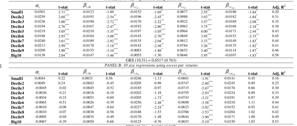
Table 3.3. 10 Size Regressions ……….. 98

Table 3.4. 25 Size and Book-to-market Regressions ………. 100

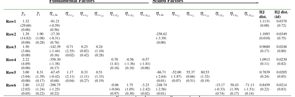
Table 3.5. Fama-MacBeth Regressions ……… 104

CHAPTER 1

INTRODUCTION

This thesis consists of two inter-connected articles that examine option

returns, and propose empirical and theoretical explanations for the

nonredundancy and allocational role of options in the economy. The first

article examines whether volatility risk is priced or not, by using a measure

from the options market, i.e. zero-beta at-the-money straddle returns. The

empirical results indicate that volatility risk is time varying, and straddle

returns are important conditioning variables, i.e agents use straddle returns

in forming their expectations about returns of securities. The article also

provides alternative explanations to the size and value vs. growth anomalies.

The second article proposes to solve individuals' consumption-investment

market, and subsequently derive optimal sharing rules for each agent in the

economy. The derivation of optimal sharing rules in a rational expectations

equilibrium yields a multifactor conditional consumption capital asset

pricing model (C-CAPM), where the first factor is the change in log

aggregate consumption, and the other factors are excess returns on a bundle

of options written on the aggregate consumption. Overall, the results have

important implications both for asset pricing and for the allocational role of

options in the economy.

1.1 RELATED LITERATURE

There are four important lines of literature that sets the motivating

ground behind this thesis. These are:

i) the inadequacy of single factor asset pricing models (why do

CAPM and C-CAPM fail to explain asset prices although they have

sound theoretical backgrounds?)

ii) the notion of market completeness (when do markets become

complete and what are the possible frictions causing markets to

become incomplete?)

iii) the allocational role of options in the economy (why do we observe

so massive trading volumes in the options market if they are

iv) the implications of nonnegative wealth constraints (what are the

equilibrium consequences of nonnegative wealth constraints

regarding the agents' consumption-investment problem?).

The following four subsections go over the major articles that have

received recognition in their own categories, present their impact on the

finance literature, and relate them to this thesis study.

1.1.1 INADEQUACY OF SINGLE FACTOR MODELS

Capital asset pricing model (CAPM) of Sharpe (1964), Lintner (1965)

and Mossin (1966) have undergone a long way since its celebrated years in

mid-sixties and seventies. The power and popularity of CAPM stem from its

parsimony and elegance. By determining an asset's return with a single

factor, namely its covariance with the market return, the so-called beta, it was

theoretically possible to price all traded assets. This simple but powerful

model has received its more-than-deserved attention in the academia, and it

has been the most popular tool for both theoreticians and practitioners

compared to any other tool in the finance literature.

After the publication of Sharpe, Lintner, and Mossin articles, there

was a wave of papers seeking to relax the strong assumptions that underpin

the original CAPM. The most frequently cited modification is by Black

(1972), who shows how the model needs to be adapted when riskless

important variant is by Brennan (1970), who finds that the structure of the

original CAPM is retained when taxes are introduced into the equilibrium.

Mayers (1972) shows that when the market portfolio includes non-traded

assets, the model also remains identical in structure to the original CAPM.

The model can also be extended to encompass international investing, as in

Solnik (1974) and Black (1974). The theoretical validity of the CAPM has even

been shown to be relatively robust if the assumption of homogenous return

expectations is relaxed, as in Williams (1977). All these studies have

increased the confidence regarding the explanatory power of CAPM, or its

versions.

On the empirical side, the situation was similar. Until mid-seventies

the cross-sectional tests initiated by Black, Jensen and Scholes (1972), and

further tests by Fama and Macbeth (1973), and Blume and Friend (1973) have

not rejected zero-beta CAPM (although rejecting the original CAPM due to

the significant error term). In contrast to these confirmatory studies, the first

important criticism to CAPM was put forward by Roll (1977). Previous tests

of the CAPM examine the relationship between equity returns and beta

measured relative to an equity market index such as the S&P500. However,

Roll demonstrates that the market, as defined in the theoretical CAPM, is not

a single equity market, but an index of all wealth. The market index must

include bonds, property, foreign assets, human capital and etc., tangible or

intangible that adds to the wealth of agents in the economy. Furthermore,

market index with certainty. Thus, Roll argues that tests of the CAPM are at

best tests of the mean-variance efficiency of the portfolio that is taken as the

market proxy. But, since within any sample, there will always be a portfolio

that is mean-variance efficient; finding evidence against the efficiency of a

given portfolio tells us nothing about whether or not the CAPM is correct.

After this theoretical criticism, came a series of anomalies that have

further weakened the ground for CAPM. Now there is a vast amount of

empirical evidence that CAPM is unable to explain the cross section of

expected returns. Banz (1981) and Reinganum (1981) show that small-sized

firms earned higher returns and big-sized firms earned lower returns than

the CAPM actually predicts. Rosenberg, Reid, and Lanstein (1984) document

that the value portfolios (high book-to-market firms) tend to outperform

growth portfolios (low book-to-market firms), which contradicted with

CAPM predictions. Basu (1977) find that price-earnings ratios can explain a

better proportion of variation in securities return than the beta of a security.

Finally, Fama and French (1992) show that size, and book-to market ratios

are superior to CAPM’s beta in explaining the cross-sectional variation in

securities returns.

In the meantime, new research was pouring in from the dynamic asset

pricing literature. A key assumption in the original CAPM is that agents

make decisions for only one time period. This is an unrealistic assumption

since investors can and actually do rebalance their portfolios on a regular

Merton (1973), which is today known as intertemporal CAPM (I-CAPM).

One of Merton's key results is that the static CAPM does not in general hold

in a dynamic setting. In particular, Merton demonstrates that an agent's

welfare at any point in time is not only a function of his own wealth, but also

the state of the economy. If the economy is doing well then the agent's

welfare will be greater than if it is doing badly, even if the level of wealth is

the same. Thus the demand for risky assets will be made up not only of the

mean-variance component, as in the static portfolio optimization problem of

Markowitz (1952), but also of a demand to hedge adverse shocks to the

investment opportunity set. The upshot is that CAPM will still hold at each

point in time, but there will be multiple betas, the number of betas being

equal to one plus the number of state variables that drive the investment

opportunity set through time. Although a major breakthrough, Merton’s

analysis was at the same time disconcerting, because it runs counter to the

basic intuition of the CAPM that an asset has greater value if its marginal

contribution to wealth is greater. The reply to this problem was the

consumption CAPM.

Breeden and Litzenberger (1978), and Breeden (1979) reconciled the gap

between Merton's I-CAPM, and the classical CAPM by highlighting the

dichotomy between wealth and consumption. In an intertemporal setting,

Breeden and Litzenberger show that agents’ preferences must be defined

over consumption. The implication is that assets are valued by their marginal

became known as C-CAPM allows assets to be priced with a single beta as in

the traditional CAPM. However, in contrast to the latter, the C-CAPM’s beta

is measured not with respect to aggregate market wealth, but with respect to

an aggregate consumption flow. As Breeden states, “the higher that an asset’s

beta with respect to consumption is, the higher its equilibrium expected rate of

return”. C-CAPM has been regarded as superior to the classical CAPM, since

an asset's covariance with the marginal utility of consumption as a measure

of systematic risk is theoretically more sound than other definitions of risk.

Also, CAPM and its extensions can almost always be expressed as either

special cases of, or proxies for, the consumption-based model. Moreover, the

consumption-based framework is a simple but powerful tool for addressing

the criticisms of Merton (1973), that the static-CAPM fails to account for the

intertemporal hedging component of asset demand, and Roll (1977), that the

market return cannot be adequately proxied by an index of common stocks.

However, empirical tests of C-CAPM have proven to be

disappointing. The consumption-based model has been rejected for the U.S.

data in its representative agent formulation with time-separable power

utility [Hansen and Singleton (1982, 1983)]. Furthermore, it has performed no

better and often worse than the simple static-CAPM in explaining the cross

section of average asset returns [Mankiw and Shapiro (1986), Breeden,

Gibbons, and Litzenberger (1989), Campbell (1996), Cochrane (1996),

Ludvigson (2001) use a scaling variable,ca)y_t, as a proxy of the log of

consumption-wealth ratio, and find that conditional versions of C-CAPM

with this conditioning variable performs much better than alternative pricing

models.

Finally, there is the arbitrage pricing theory (APT), which is an

attempt to resolve the inadequacies in single factor models. It is no surprise

that Ross (1976) has developed his model almost at the same time with Roll's

critique, and the first reported anomalies. While still retaining the core idea

of CAPM (covariance of an asset's return with a number of factors are the

determinant of the long term average return of that security), the major

contribution of the model is its allowance to multiple factors in pricing of

securities. Although the choice of appropriate factors still being debated, and

there is no clear-cut methodology to which factors should be included, the

model's strength comes from the broadness of its assumptions and its

testability. Once you define theoretically appropriate factors that affect an

asset's return systematically, then APT is relatively superior to classical

single factor models.

1.1.2 ARE MARKETS (IN)COMPLETE?

Financial economics deals with agents' decision making (i.e. optimal

The general framework of decision making under uncertainty has been

established by the seminal works of Arrow (1951, 1953), Debreu (1951), and

Arrow and Debreu (1954). These studies have chosen to model uncertainty as

the revelation of a state of the world. Individuals in these models face

investment and consumption decisions based on payoffs of securities that

vary across different states of the world. The basic building blocks of the

state-preference theory are the event state-contingent claims. A

time-event state-contingent claim is a contract that promises to deliver to the

holder of that contract a particular commodity when a particular state occurs

at a particular time, and delivers nothing at any other state and/or time.

Agents maximize their utilities over these time-event state-contingent claims.

The Arrow-Debreu framework has two versions: a state-contingent

claims model, and a securities market model. The notion of market

completeness refers to having a complete set of state-contingent claim

markets in the first version (i.e. each state-contingent claim can be priced in

these markets at the beginning of the trade); and number of linearly

independent securities being equal to the number of states in the second

version. In complete markets, the resulting equilibrium is such that each

agent purchases a set of future state-contingent commodities in the initial

time period, and then just watches the future states and events unfold.

Since Arrow-Debreu equilibrium conditions are oversimplified

versions of the general uncertainty in the economy, following research

economy. The result was a sequential equilibrium framework, where three

different versions emerged: temporary equilibrium by Stigum (1969), and

Grandmont and Hildenbrand (1974); Radner equilibrium by Radner (1972),

and rational expectations equilibrium by Lucas (1972), and Green (1973). In

the classical Arrow-Debreu equilibrium, once we have complete markets

there is no need for markets to reopen. All trading takes place at the initial

period, and then there is no need for trading in subsequent periods. All the

three equilibria mentioned above have the same common characteristic, i.e.

spot markets and securities markets are open in the sequences following the

initial period. The essential distinctions between these theories lie in the form

of expectations assumed, i.e. temporary equilibrium does not require perfect

foresight, or information-consistency across agents; Radner equilibrium

requires perfect foresight, but not consistency; and rational expectations

equilibrium require information-consistent expectations. The framework in

the second article will be a rational expectations framework with incomplete

markets. So it is of importance to further discuss these two concepts and

relate them to the setting of this thesis.

A rational expectations equilibrium can be thought of as the special

case of the Radner equilibrium when the probabilities assigned by all agents

about future states are the same across agents. More specifically, agents are

assumed to form "information-consistent" probability assignments. As long

as agents have the same information about the future of the economy, then

assumed that all agents share a common information structure,

{

}

F _{= t}, ₌0,1,K, _{, where each}

t

F is a partition of the state space Ω . Thus,

as information is revealed at each period, each agent knows what state she is

in, and forms the same probabilistic assignments with other agents regarding

the future possibilities of events.

The basic idea behind incomplete markets is the possibility of having a

sequential economy where there are an insufficient number of financial

securities. Specifically, markets are said to be incomplete if the number of

linearly independent securities is strictly less than the number of possible

future states. Although a general Radner equilibrium can still be attained in

incomplete markets, the allocation among agents is no more Pareto efficient.

The markets in the second article are incomplete given the total number of

traded securities, and the consumption patterns of agents. However, once

options are introduced, markets are effectively completed and an efficient

allocation among agents is achieved. This relates the issue to the allocational

role of options in incomplete markets, which is the subject of next section.

1.1.3 ALLOCATIONAL ROLE OF OPTIONS

According to Bank of International Settlements, the size of derivatives

markets in 2002 was estimated to exceed $109 trillion in outstanding

Today, the daily trading volumes on currency exchanges are on average $3.5

trillion dollars, much ahead of the spot market transaction volumes. What do

these numbers mean about the allocational role of options in the economy? If

options are redundant securities as implied by Black-Scholes assumptions,

why do we observe huge amounts of options trading in the economy. The

answer can not solely relay on hedging purposes or speculation. Today,

many researchers question the redundancy of options, and there is a growing

amount of literature on the spanning role of options.

The elegant option pricing theory developed by Black and Scholes

(1973) relies on a simple rule; the replication of an option's payoff with that

of a risky asset and a riskless asset. This no arbitrage condition implies that

options are redundant securities, and have no allocational role in the

economy. The first study that shows how standard call and put options can

be used to complete a securities market goes back to the seminal work of

Ross (1976). Ross shows that when the markets are incomplete, one can

construct options with prespecified strike prices to span the state space. In

the same spirit with this study, Breeden and Litzenberger (1978) show that

constructing options whose strike prices coincide with every possible level of

aggregate wealth are sufficient to characterize the prices of Arrow-Debreu

securities.

The idea of market completion by options has been carried further to a

multiperiod setting by Kreps (1982), and Duffie and Huang (1985). They

long-lived securities. This implies that the number of long-lived securities

needed to complete markets is far fewer than the total number of states, i.e. it

is just equal to the number of branches leaving each node on the event tree

representing the information structure. Thus by dynamically trading

long-lived securities markets can be completed, and a Pareto optimal allocation

can be achieved.

The above theoretical research had significant impact on option

pricing literature. Although standard Black-Scholes option pricing model is

still widely used in practice, research today has shifted from assuming

complete markets to examining the settings of why and how markets become

incomplete, focus on the allocational consequences of market

incompleteness, and develop alternative option pricing models. The

following sub-sections analyze different settings that can cause markets to be

incomplete, and summarize recent findings in these settings,

correspondingly.

1.1.3.1 Heterogeneous Beliefs

This line of research argues that heterogeneous attitudes towards risk

can generate demand for options. For example, Leland (1980) shows that in

an economy with terminal consumption only, convex final payoffs such as

options will be demanded by more risk-tolerant agents. Grosmann and Zhou

averse to the risk when his wealth drops below a given threshold, than the

demand for options can be an important determinant of the underlying asset

price. Bates (2001) considers an economy where crashes can occur and less

crash-tolerant investors buy options from more crash-tolerant ones. In his

setting, options complete the market by serving as a hedge against crash risk.

Buraschi and Jiltsov (2003) consider a symmetric but incomplete information

setting; agents agree on the dividend process but differ in their beliefs about

the price process unrelated to fundamentals. They find that much of the

observed option trading volume can be explained by this heterogeneity in

beliefs.

1.1.3.2 Asymmetric Information

Asymmetric information about the dividend process can induce

traders with private information to hold options in equilibrium. A number of

studies suggest that option may be non-redundant because the price of a

traded option can convey some information, which otherwise would be

unobservable in the economy. Grossman (1988) argues that an option may

appear to be redundant, however it can be nonredundant due to its

informational content, thus its removal from the economy would make

markets incomplete. Back (1993) shows that the introduction of option

trading into a market with asymmetric information may change the

a complete market may become non-redundant. Also Easley, O’Hara, and

Srinivas (1998) suggest that an option market could be a platform for

informed trading due to lower transaction costs and greater financial

leverage.

1.1.3.3 Stochastic Volatility and Jumps

Presence of stochastic volatility and jumps can severely affect asset

prices and thus options that are written on them. The main approach to

modeling stock returns is defining a continuous time stochastic volatility

diffusion process possibly augmented with an independent jump process in

returns. Today, most option pricing models incorporate these two factors in

order to account for a more realistic pricing process. It was first Heston

(1993) who proposed a stochastic volatility diffusion model, for which one

could analytically derive an option pricing formula. Duffie and Kan (1996),

and Duffie, Pan, and Singleton (2000) further developed Heston's model to a

rich class of affine jump diffusion processes. Several other authors have used

stochastic volatility diffusion process augmented by jumps [Bates (1996)

Andersen, Benzoni and Lund (2001), Eraker, Johannes and Polson (2001), Pan

(2002), Chernov, Gallant, Ghysels and Tauchen (2003)]. Bakshi, Cao, and

Chen (1997) compare empirical performances of these alternative option

pricing models with respect to three criteria; internal consistency of implied

hedging performance. Overall, models that include stochastic volatility and

jump processes perform the best.

Besides these theoretical models, recently, a number of empirical

papers have demonstrated that options are not redundant. Buraschi and

Jackwerth (2001) test whether the pricing kernel of the economy can be

spanned by stock and bonds or whether additional securities are required.

Their results suggest that option returns do significantly increase the

spanning quality of the pricing kernel and that the volatility risk is priced.

Coval and Shumway (2001) give preliminary evidence that returns on

zero-beta at-the-money straddles can explain a significant amount of S&P 100

index returns, and argue that at-the-money straddles can account for the

systematic volatility risk in the securities market. Bakshi and Kapadia (2003)

show that delta-hedged option portfolios consistently earn negative returns,

indicating that there exists a negative volatility risk premium in option

prices, which is consistent with the nonredundancy of options. Liu and Pan

(2003) argue that, in the existence of volatility and jump risks, a market

consisting of a riskless bond and a risky asset is not enough to replicate the

possible payoffs resulting from those risks, thus the markets are strongly

incomplete. They show that at-the-money straddles and out-of-money puts

can be used to complete the markets and derive optimal demands for those

1.1.3.4 Market Frictions

The standard asset pricing and option pricing theories assume that

markets are frictionless, i.e. no transaction costs, no limitations on short sales,

or borrowing. However, real-life practice seldom approves these cases. The

presence of transaction costs, and portfolio constraints such as constraints on

short selling, or credit constraints such as nonnegative wealth constraints can

generate demand for options, and options can have important allocational

roles due to those frictions in the economy.

Regarding the transaction costs, Lee and Yi (2001) test whether greater

leverage and lower trading costs make options more attractive to informed

traders, and if the relative lack of anonymity in options markets discourages

large investors from trading options. They find that the adverse selection

component of the bid-ask spread decreases with option delta, implying that

options with greater financial leverage attract more informed investors. Kaul,

Nimalendran, and Zhang (2002) examine the relation between adverse

selection in the underlying stock and spreads on options of different strike

prices. Their main finding is that adverse selection costs are highest for

at-the-money options. The authors argue that this result is consistent with the

trade-off between high leverage and transaction costs. In Basak and Croitoru

portfolio constraints on short selling and investors with heterogeneous

beliefs. The degree of mispricing and optimal derivative portfolio holdings

becomes non-trivial in their generalized equilibrium framework. Vanden

(2004) examine the effect of nonnegative wealth constraints in a single period

economy, and in equilibrium agents hold options thus options become

nonredundant. The markets are strongly incomplete given the traded

options, but options help agents achieve a Pareto efficient allocation, and in

equilibrium, options effectively complete the market. Since, in equilibrium,

agents agree on the value of all stochastic payoffs, Vanden's findings have

important consequences for asset pricing. This is because the payoffs from

existing securities (a positive probability of bankruptcy) in addition to the

short selling possibilities can lead agents reach negative levels of wealth.

Hence, by imposing nonnegative wealth constraints agents are guaranteed to

come back to the economy with the ability to repay their debt. The economic

intuition and related literature regarding nonnegative wealth is the subject of

the next sub-section.

1.1.4 NONNEGATIVE WEALTH CONSTRAINTS

As noted in the previous sub-sections, frictionless markets assumption

breaks down in real life practices. There may be some constraints on wealth

(or borrowing limits), which can practically affect individuals' optimal

Dybvig and Huang (1988), or nonnegative wealth by Vanden (2004) might

force individuals to alter their unconstrained optimal solutions, which can

result in certain payoffs that cannot be replicated by the existing financial

instruments.

The analysis of nonnegative wealth constraints and their implications

on individual's consumption-investment decision and option pricing goes

back to Harrsion and Kreps (1979). In their pioneering work, in a continuous

time setting, it is demonstrated that doubling strategies (which refers to one's

doubling her bet at a roulette game) can earn arbitrage profits in a finite time

interval. Since the core of investment-consumption decision and option

pricing rests on the no-arbitrage condition, the existence of doubling

strategies, thus arbitrage opportunities, precludes having a solution to the

optimal investment-consumption problem, and obviously invalidates the

option pricing theory. Harrison and Kreps conjecture that arbitrage

possibilities are ruled out if trading strategies are restricted to those having

nonnegative wealth at all times. Dybvig and Huang (1988) generalize their

work in assuming a lower bound on wealth. This assumption is economically

plausible since there are institutional restrictions on the amount of credit an

individual can borrow. They show that any lower bound on wealth rules out

doubling strategies, and any other strategies that generate a free lunch.

The effect of nonnegative wealth constraint on individual's optimal

consumption-investment problem has been studied by Cox and Huang

equilibrium framework by Vanden (2004). Although the previous studies

examine the problem by considering a single individual's

consumption-investment decision framework, the results derived by Vanden assume that

all agents simultaneously face nonnegative wealth constraints. The results

have important allocational implications regarding the individuals' optimal

consumption-investment decisions.

Overall, the above literature can be summarized as follows:

i. Single factor models of asset pricing fail to explain the cross

sectional variation in securities returns.

ii. Markets are incomplete due to several real life frictions and

options can be used effectively to complete markets, making

them non-redundant securities.

iii. An asset pricing model that takes into account theoretical

weaknesses in i and ii, is theoretically more sound, and

resembles reality better.

This thesis combines the above asset pricing literature, and examines

two asset pricing models that are theoretically sound, and empirically

testable. The first article proposes a single factor conditional CAPM where

straddle returns are used as a conditioning variable, and the second article

proposes a multifactor conditional C-CAPM where option returns appear as

factors. To the best of our knowledge, the first article is the first study that

uses straddle returns in the context of volatility risk, and the second article is

Overall the tested models provide some supportive evidence for the

nonredundancy, and allocational role of options in the economy.

CHAPTER 2

IS VOLATILITY RISK PRICED IN THE SECURITIES

MARKET? EVIDENCE FROM S&P 500 INDEX OPTIONS

2.1 INTRODUCTION AND LITERATURE REVIEW

The notion that equity returns exhibit stochastic volatility is well

documented in the asset pricing literature.1 _{Furthermore, recent evidence}

indicates the existence of a negative volatility risk premium in the options

market [Lamoureux and Lastrapes (1993), Buraschi and Jackwerth (2001),

Coval and Shumway, (2001), Bakshi and Kapadia (2003)]. However, the

existence of volatility risk in the securities market and its impact on different

1

See Engle and Ng (1993), Canina and Figlewski (1993), Duffee (1995), Braun, Nelson, and Sunier (1995), Andersen (1996), Bollerslev and Mikkelsen (1999), and Bekaert and Wu (2000).

classes of firms has not been extensively documented. Recently, Coval and

Shumway (2001) examines the return characteristics of S&P 100 index

straddles and gives preliminary evidence that volatility risk may be a

common risk factor in securities markets - a finding that contradicts the

classical CAPM.

CAPM suggests that the only common risk factor relevant to the

pricing of any asset is its covariance with the market portfolio; thus an asset's

beta is the appropriate quantity for measuring the risk of any asset.

However, Vanden (2004) shows that when agents face nonnegative wealth

constraints, cross sectional variation in securities returns is not explained

only by an asset's beta. Instead, excess returns on the traded index options

and on the market portfolio explain this variation; implying that options are

nonredundant securities. Furthermore, as Detemple and Selden (1991)

suggest, if options in the economy are non-redundant securities, then there

should be a general interaction between the returns of risky assets and the

returns of options. This implies that option returns should help explain

security returns.

This article extends the preceding studies and presents evidence that

straddle returns are important for asset pricing since they help capture time

variation in the stochastic discount factor. The findings suggest that volatility

risk is time-varying and that options are nonredundant securities at volatile

states of the economy. This has important implications regarding the

regressions, Fama-MacBeth regressions, and GMM-SDF estimations in this

article confirm the theory that options are effective tools in pricing securities

and allocating wealth among agents as suggested by Vanden (2004). This

article also examines the effect of volatility risk in pricing different classes of

firms, i.e. small vs. big and value vs. growth, and finds distinct patterns in

the returns of these firms, especially at volatile states of the economy.

Asset pricing theories thus far have been unable to provide a

satisfactory economic explanation for the size and value vs. growth

anomalies.2 _{In a rational markets framework, we would expect these}

abnormal returns to be temporary. Once investors realize arbitrage

opportunities, the abnormal profits of small and value stocks are expected to

vanish. However, this has not been the case. The persistence of these two

anomalies has led to extensive research and has yielded two alternative lines

of explanations within the rational markets paradigm.

One line, led by Fama and French (1992, 1993, 1995), argues that a

stock's beta is not the only risk factor. This approach suggests that

fundamental additional variables such as book-to-market and market value

explain equity returns much better, because they are proxies for some

unidentified risk factors. However, the weakness of this explanation lies in

its failure to address the economic variables underlying these factors. The

2

Banz (1981) and Reinganum (1981) document that portfolios formed on small sized firms earn returns higher than the CAPM predicts. Rosenberg, Reid and Leinstein (1985) find that firms with high book-to-market ratios (value firms) earn higher returns than firms with low book-to-market ratios (growth firms). Davis, Fama, and French (2000) report that the value premium in U.S. stocks is robust.

other line of research within the risk-return framework argues that it is the

time variation in betas and the market risk premium that cause the static

CAPM to fail to explain these anomalies. There is now considerable evidence

that conditional versions of CAPM perform much better than their

unconditional counterparts.3

This article re-examines these two important asset pricing anomalies

with an important but somewhat overlooked factor, the volatility risk. There

is now a considerable amount of evidence that volatility risk is priced in the

options market. First, Jackwerth and Rubinstein (1996) report that

at-the-money implied volatilities of call and put options are consistently higher

than their realized volatilities, suggesting that a negative volatility premium

could be an explanation to this empirical irregularity. Furthermore, Coval

and Shumway (2001) report that zero-beta at-the-money straddles on the

S&P 100 index earn returns consistently lower than the risk free rate,

suggesting the presence of a negative volatility risk premium in the prices of

options. As an extension of this study, Driessen and Maenhout (2005) report

that volatility risk is also priced in FTSE and Nikkei index options. Finally,

Bakshi and Kapadia (2003) show that delta-hedged option portfolios

consistently earn negative returns and conclude that there exists a negative

volatility risk premium in option prices.

3

See Ferson (989), Ferson and Harvey (1991), Ferson and Korajczyk (1995), Jagannathan and Wang (1996), Lettau and Ludvigson (2001), and Altay-Salih, Akdeniz, and Caner (2003) for the theory behind time-varying beta and conditional CAPM literature.

Although the above evidence indicates that volatility risk is priced in

options markets, we are less confident that it is priced in securities markets.

Recent studies find that volatility risk can explain the cross-section of

expected returns. For example, Moise (2005) uses innovations in the realized

stock market volatility, and demonstrate that volatility risk helps explain

some of the size anomaly. Furthermore, by using changes in the volatility

index (VIX) of Chicago Board Options Exchange (CBOE), Ang, Hodrick,

Xing, and Zhang (2006) demonstrate that aggregate volatility is a

cross-sectional risk factor. In this study, a measure from the options market, i.e.

straddle returns on the S&P 500 index, is used as a proxy for volatility risk.

The reason behind using straddle returns is intuitive. As Detemple and

Selden (1991) argue, if options are non-redundant securities in the economy,

then their returns should appear as factors in explaining the cross section of

asset returns. Furthermore, Vanden (2004) reports that returns of call and put

options indeed explain a significant amount of variation in securities return,

but fail to explain the returns for small and value stocks. The failure of

Vanden's model could be due to omitting an important risk factor - the

volatility risk. Furthermore, straddles are volatility trades, and they provide

insurance against significant downward moves.4 _{Thus, overall, straddle}

returns are ideal for studying the effects of volatility risk in security returns.

4

This is because increased market volatility coincides with downward market moves, a phenomenon which is reported by French, Schwert, and Stambaugh (1987), and Glosten, Jagannathan, and Runkle (1993). Engle and Ng (1993) show that volatility is more associated with downward market moves due to the leverage effect.

The remainder of this article is organized as follows. First, data and

the methodology for calculating straddle returns are presented. Econometric

issues in the estimation of the volatility risk premium are discussed in the

next section. This is followed by empirical results. The final section offers

concluding remarks.

2.2 DATA AND METHODOLOGY

The data consist of two parts - S&P 500 options data and stock return

data - covering the period January 1987 through October 1994.5 _{Daily S&P}

500 options data is obtained from the Chicago Board Options Exchange and

consists of daily closing prices of call and put options, the daily closing level

of the S&P 500 index, the maturities and strike prices for each option, the

dividend yield on the S&P 500 index, and the one-month T-bill rate. For

option volatilities, the closing level of CBOE's S&P 500 VIX index is used. For

market portfolio, CRSP’s value weighted index on all NYSE, AMEX and

NASDAQ stocks are used. The return data on size and book-to-market

portfolios are obtained from Kenneth French's data library.

The method for calculating daily option returns is as follows. First,

options that significantly violate arbitrage-pricing bounds are eliminated.

Then, options that expire during the following calendar month are identified.

5

This roughly coincides with options that have 14 to 50 days to expiry in our

sample. The reason for choosing options that expire the next calendar month

is that they are the most liquid data among various maturities.6 _{Options that}

expire within 14 days are excluded from the sample, because they show large

deviations in trading volumes, which casts doubt on the reliability of their

pricing associated with increased volatility.7 _{Next, each option is checked}

whether it is traded the next trading day or not. If no option is found in the

nearest expiry contracts, then options in the second-nearest expiry contracts

are used. To calculate the daily return of an option, raw net returns are used.

The usage of raw net returns is justified by Coval and Shumway (2001) who

argue that log-scaling of option returns can be quite problematic.

Once daily call and put returns are calculated, they are grouped

according to their moneyness levels. Although there is no standard

procedure for classifying at-the-money options, options with a moneyness

level (S-K) between -5 and +5 are classified as at-the-money options. This

classification also guarantees that there are at least two options around the

spot price. One reason for focusing on zero-beta at-the-money straddles was

to capture the effect of volatility risk, as mentioned previously. Another

advantage of studying at-the-money options is that they are less prone to

pricing errors compared to deep-out-of money options, as cited in option

6

According to Buraschi and Jackwerth (2001), most of the trading activity in S&P500 options is concentrated in the nearest (0-30 days to expiry) and second nearest (30-60 days to expiry) contracts.

7

pricing literature.8 _{Using the above procedure results in 1937 days of return}

data out of 1980 trading days.

The straddle returns are calculated according to the methodology

outlined by Coval and Shumway (2001). In order to capture the effect of

volatility risk, zero-beta at-the-money straddle returns on the S&P 500 index

are used. The advantage of using S&P 500 index options is that they are

highly liquid, thus they are less prone to microstructure and illiquid trading

effects. Zero-beta straddles are formed by solving for θ from the following set

of equations,

(

)

(

)

where rv is the straddle return, rc and

r

the fraction of the straddle’s value in call options, and βc and βpare the

market betas of the call and put options, respectively. It is straightforward to

calculate returns on call and put options; however, to calculate the return of a

straddle, the value of θ is needed, which depends on β_c and βp. By using the

put-call parity theorem, Equation (2) can be reduced into a single unknown,

c

β , and the value of θ is derived as follows

8

Macbeth and Merville (1979) report that the Black-Scholes prices of at-the-money call options are on average less than market prices for in-the-money call options. Also, Gencay and Salih (2001) document that pricing errors are larger in the deeper-out-of-money options compared to at-the-money options.

s C P s C c c c + − + − = β β β θ (3)

where C is price of the call option, P is price of the put option, and s is the

level of the S&P 500 index.

The only parameter that is not directly observable in the above

equation is the call option’s beta, βc. We use Black-Scholes' beta, which is

defined as c

(

)

(

)

where N[.] is the cumulative normal distribution, X is the exercise price of

call option, r is the risk-free short term interest rate, q is the dividend yield

for S&P 500 assets, σ is the standard deviation of S&P 500 returns, and t is the

option's time to maturity.

The methodology to calculate zero-beta at-the-money straddle returns

is as follows. First, an option's beta is calculated according to Equation (4).

Then, θ is derived by incorporating the previously calculated call and put

option returns into Equation (3). Finally, straddle returns for each day are

calculated according to Equation (1). The daily zero-beta straddle return is

then simply the equally-weighted average of at-the money-straddle returns

that are found in the final step.

Table 2.1 reports the summary statistics for the daily S&P 500 (SPX)

minimum return of –87.77% and maximum of 441.79%. The mean and

median of the daily zero-beta straddle returns are negative as documented

by the earlier literature. Note that call option betas are instantaneous betas,

and therefore the straddles are zero-beta at the construction. However, we

calculate the zero-beta straddle returns by using daily buy and hold returns.

Thus, they are zero-beta instantaneously and their betas might change

during the holding period. This might be the possible explanation of

negative correlation of -0.54 between the straddle and market returns.9

TABLE 2.1

Summary Statistics for Daily Zero-Beta Straddles

Daily Straddle Returns (%)

Mean -1.06 Median -1.58 Minimum -87.77 Maximum 441.79 Skewness 17.03 Kurtosis 520.03 Correlation -0.54

Note. This table reports the summary statistics for the returns of daily zero-beta at-the money straddles. The sample covers the period January 1987 to October 1994 (1980 days). After adjusting for moneyness and maturity criteria, we end up with 1937 days of data. Correlation is the correlation of straddle returns with market returns.

2.3 ECONOMETRIC SPECIFICATIONS

In order to test the main hypothesis that volatility risk - proxied by

zero-beta at-the-money straddle returns - is priced in securities returns, we

9

To check the robustness of the results, we set the theoretical position beta in Equation (2) to a constant such that the in-sample straddle beta is exactly zero. Negative mean and median volatility risk premium still persists and furthermore conclusions from time series regressions do not change.

first regress the excess returns of size and book-to-market portfolios on

excess straddle returns and on the market factor.10 _{The empirical model to be}

tested is

(

)

∑

where rit's are realized returns of size and book-to-market portfolios, and rjt's

are the returns of factors that are included in the regressions.

The above analysis relies on monthly holding period returns, both

because microstructure effects tend to distort daily returns, and to rule out

non-synchronous trading effects that could be present in daily data. In order

to calculate monthly at-the-money straddle returns, an equally weighted

portfolio of at-the-money straddles is formed for each day and then each

day's return is cumulated to find monthly holding period returns. This adds

up to 94 monthly straddle returns, which are used as an independent

variable in the preceding time-series regressions. Although these regressions

are not formal tests of whether volatility risk is priced or not, they

nevertheless give clues about the potential explanatory power of straddle

returns in explaining the cross-section of expected returns.

Next the question of whether volatility risk is a priced risk factor is

examined by performing Fama-MacBeth two-pass regressions by using the

25 size and book-to-market portfolios.11 _{The model to be tested is}

10

Vanden (2004) uses a similar model, where he includes call and put option returns and a market factor as explanatory factors.

11

E

[ ]

More specifically, in the first pass, portfolio betas are estimated from a

single multiple time-series regression via Equation (5). Instead of using the

5-year rolling-window approach, a full sample period is used.12 _{In the second}

pass, a cross-sectional regression is run at each time period, with full-sample

betas obtained from the first pass regressions, i.e.

E

[ ]

Fama and MacBeth (1973) suggests that we estimate the intercept term

and risk premia, αiand λj's, as the average of cross-sectional regression

estimates

∑

∑

One problem with the Fama-MacBeth procedure is that it ignores the

errors-in-variables problem that results from the fact that in the second pass,

beta estimates instead of the true betas are used. In order to avoid this

problem, a Generalized Method of Moments (GMM) approach within the

stochastic discount factor (SDF) representation is employed. The advantage

of a GMM approach is that it allows the estimation of model parameters in a

single pass, thereby avoiding the errors-in-variables problem. The advantage

of the SDF representation relative to the beta representation is that it is

12

extremely general in its assumptions and can be applied to all asset classes,

including stocks, bonds, and derivatives. Cochrane (2001) demonstrates that

both representations express the same point, but from slightly different

viewpoints. However, the SDF view is more general, it encompasses virtually

all other commonly known asset pricing models. Ross (1976) and Harrison

and Kreps (1979) state that in the absence of arbitrage and when financial

markets satisfy the law of one price, there exists a stochastic discount factor,

or pricing kernel, mt+1, such that the following equation holds

[

]

E , (8)

where Rit+1 is the gross return (one plus the net return) on any traded asset i,

from period t to period t+1. We denote this as the unconditional SDF model.

Because considerable evidence exists to suggest that expected excess

returns are time-varying, the above unconditional specification may be too

restrictive. Thus, to answer the question of whether or not there exists

time-variation in the volatility risk premium, both unconditional and conditional

models of asset pricing are tested. The conditional SDF model is denoted as

[

]

t R m

E (9)

where Et denotes the mathematical expectation operator conditional on the

information available at time t.

Following Jagannathan and Wang (1996), we consider a linear factor

pricing model with observable factors, ft. Then, mt+1 can be represented as

where at, and bt are time-varying parameters. Note that, when at, and bt are

constants, we obtain the unconditional version of linear factor models.

The question here is how one can incorporate the information that

investors use when they determine expected returns in Equations (9) and

(10). Because the investors' true information set is unobservable, one has to

find observable variables to proxy for that information set. Cochrane (1996)

shows that conditional asset pricing models can be tested via a conditioning

time t information variable, zt. One way of incorporating conditioning

variable, zt, into the model is to scale factor returns, as discussed in Cochrane

(2001); and used in Cochrane (1996), Hodrick and Zhang (2001), and Lettau

and Ludvigson (2001b). This is done by scaling the factors with zt, thus

modeling the parameters at, and bt as linear functions of zt as follows

t t z a =γ₀ +γ₁ (11) t t z b =η₀+η₁ (12)

Plugging these equations into Equation (10), and assuming that we

have a single factor, we have a scaled multifactor model with constant

coefficients taking the form

mt+1 =

(

) (

)

=γ₀ +γ₁zt +ηoft+₁+η₁ztft+₁ (13)

The scaled multifactor model can be tested by rewriting the

conditional factor model in Equation (9), as an unconditional factor model

E

[

(

)

]

In the next section, empirical results of OLS time-series regressions

(Equation 5), Fama-MacBeth regressions (Equation 6), and the GMM-SDF

estimations (Equation 8) are presented.

2.4 EMPIRICAL FINDINGS

2.4.1 TIME SERIES REGRESSIONS

Coval and Shumway (CS; 2001) argue that zero-beta at-the-money

straddles can proxy for volatility risk, which can in turn explain the variation

in the cross-section of equity returns. Usually, highly volatile periods are

associated with significant downward market moves. Furthermore, index

straddles earn positive (negative) returns in times of high (low) volatility, as

can be seen by the negative correlation between the straddle and market

returns in Table 2.1. CS also argue that volatility risk is a possible explanation

for the well-known size anomaly among securities returns. For a preliminary

investigation of those two hypotheses, we use a two-factor model, and

regress excess returns of CRSP's size deciles on the excess returns of CRSP's

value-weighted index on all NYSE, AMEX, and NASDAQ stocks and the

excess returns of zero-beta at-the-money straddles. Table 2.2 presents the

TABLE 2.2

2-Factor Time Series Regressions

rit - rft = αi + βim (rmt -rft) + βiv (rvt -rft) +εit

rit - rf αi t-statistic βim t-statistic βiv t-statistic Adj. R2

Small 10 -0.0024 -0.61 0.7555 6.91*** -0.0109 -4.55*** 0.64 Decile 9 -0.0039 -1.23 0.9612 11.37*** -0.0080 -4.29*** 0.78 Decile 8 -0.0004 -0.18 1.0106 13.69*** -0.0063 -3.98*** 0.84 Decile 7 -0.0017 -0.70 1.0612 14.86*** -0.0052 -3.33*** 0.86 Decile 6 0.0009 0.40 1.0553 14.83*** -0.0040 -2.74*** 0.88 Decile 5 0.0009 0.51 1.0337 20.91*** -0.0031 -3.02*** 0.92 Decile 4 0.0004 0.37 1.0343 27.10*** -0.0024 -2.31** 0.95 Decile 3 0.0007 0.60 1.0917 27.76*** 0.0003 0.36 0.96 Decile 2 0.0004 0.55 1.0801 34.26*** 0.0019 2.67*** 0.98 Big 1 0.0006 0.56 0.9953 32.97*** 0.0024 2.99*** 0.96 GRS F-Test = 2.3314 (p=0. 0179)

Note. This table reports monthly time-series regression results of excess returns of CRSP's size deciles on market factor and excess straddle returns. The dependent variable is the excess return of CRSP's size-decile portfolio, rmt is the return of CRSP's value-weighted index on all NYSE, AMEX, and

NASDAQ stocks, , rvt, is the monthly zero-beta straddle return, and rf is the 1-month T-bill rate. ***, **

, * denote 0.01, 0.05, and 0.10 significance levels, respectively. All t-values are corrected for autocorrelation (with lag=3) and heteroskedasticity as suggested by Newey and West (1987). GRS F-Test reported at the bottom of the table is from Gibbons, Ross, and Shanken (1989).

As can be seen from the table, there exists a statistically significant

relationship between straddle returns and securities returns in 9 of the 10

size deciles. Thus, straddle returns and therefore volatility risk could be a

significant variable in explaining securities returns. In their recent studies,

Moise (2005) and Ang et al. (2006) also document statistically significant

negative price of risk for aggregate volatility. In our case, the economic

interpretation of this negative volatility risk premium could be that buyers of

zero-beta at-the-money straddles are willing to pay a premium for downside

market risk. If investors are assumed to be averse to downward market

moves, the existence of a negative volatility risk premium would be justified,

because downward moves are associated with high volatility periods.