Inter-regional connectivity in the human brain during visual search

(1)

INTER-REGIONAL CONNECTIVITY IN THE

HUMAN BRAIN DURING VISUAL SEARCH

a thesis submitted to

the graduate school of engineering and science

of bilkent university

in partial fulfillment of the requirements for

the degree of

master of science

in

electrical and electronics engineering

By

Salman Ul Hassan Dar

August, 2016

(2)

Inter-Regional Connectivity in the Human Brain During Visual Search By Salman Ul Hassan Dar

August, 2016

We certify that we have read this thesis and that in our opinion it is fully adequate, in scope and in quality, as a thesis for the degree of Master of Science.

Tolga C¸ ukur(Advisor)

Emine ¨Ulk¨u Sarıta¸s

Fato¸s Yarman Vural

Approved for the Graduate School of Engineering and Science:

Levent Onural

(3)

ABSTRACT

INTER-REGIONAL CONNECTIVITY IN THE HUMAN BRAIN

DURING VISUAL SEARCH

Salman Ul Hassan Dar

M.S. in Electrical and Electronics Engineering Advisor: Tolga C¸ ukur

August, 2016

Separate groups of regions in the human brain are thought to be functionally specialized for representing specific categories of visual objects, and for controlling and deployments of visual attention. It is commonly assumed that the information flow between these regions is altered during visual search. However, little is known about the magnitude and extent of these changes during natural visual search. Here, we assess the changes in functional con-nectivity between the attention-control network and the category-selective regions during category-based visual search in natural movies. Brain activity was recorded using functional magnetic resonance imaging (fMRI) while subjects viewed natural movies.

To investigate the changes in connectivity strength between pairs of brain regions, we em-ployed coherence analysis. Coherence is a non-directional measure of association, which identifies correlation in frequency domain. To infer the influence of attention-control areas on category-selective areas, Granger causality analysis was carried out. Granger causality uses the idea of temporal precedence that cause precedes the effect. Furthermore, to exam-ine whether attention changes inter-regional connectivity after accounting for stimulus-driven brain activity, two separate encoding models were used to capture brain responses elicited by low-level structural and high-level category features in natural movies via L2-regularized linear regression. Response predictions of the structural and category models were removed from the recorded blood-oxygen-level dependent (BOLD) responses to obtain the residual responses. The connectivity analyses were repeated on the residuals to determine if the at-tentional changes in connectivity persist even after projecting out the stimulus-driven brain activity.

The results indicate that performing visual search for a specific object category enhances the influence of high-level attention-control network on category-selective areas in ventral temporal cortex. Furthermore, these connectivity patterns persist even after projecting out the stimulus-driven brain activity from the recorded BOLD responses.

(4)

¨

OZET

G ¨

ORSEL D˙IKKAT SIRASINDA ˙INSAN BEYN˙INDEK˙I

B ¨

OLGELER-ARASI BA ˘

GLANTILILIK

Salman Ul Hassan Dar

Elektrik Ve Elektronik Mühendisli˘gi, Yüksek Lisans Tez Danı¸smanı: Tolga Ç ukur

A˘gustos 2016

˙Insan beynindeki farklı bölgelerin, görsel nesne sınıflarını temsil etmek ve görsel dikkati kon-trol edip düzenlemek i¸cin i¸slevsel olarak özelle¸sti˘gi dü¸sünülmektedir. Bu bölgeler arasındaki bilgi akı¸sının görsel arama sırasında de˘gi¸sime u˘gradı˘gı dü¸sünülmektedir. Yine de, görsel arama sırasında olu¸san bu de˘gi¸sikliklerin büyüklü˘gü ve kapsamı yeterince bilinmemektedir. Bu tezde, do˘gal film sahneleri izlenirken sınıf-temelli görsel arama sırasında dikkat-kontrol a˘gı ve sınıf-se¸cici bölgeler arasındaki i¸slevsel ba˘glantıların de˘gi¸simlerini de˘gerlendirmekteyiz. Denekler do˘gal filmleri izlerken beyin aktiviteleri i¸slevsel manyetik rezonans görüntüleme (fMRI) ile kaydedildi.

Farklı beyin bölgesi ¸ciftlerinin ba˘glantı miktarlarındaki de˘gi¸simi incelemek i¸cin uyumluluk analizleri uyguladık. Uyumluluk, frekans uzayındaki ili¸skiyi belirten, ba˘glantının yönsüz bir öl¸cütüdür. Dikkat-kontrol bölgelerinin sınıf-se¸cici bölgelere olan etkisini anlamak i¸cin Granger nedensellik analizi yapıldı. Granger nedenselli˘gi zamansal öncüllük ilkesini kullanır: Neden sonuca göre zamansal olarak öndedir. Ayrıca, dikkatin bölgeler-arası ba˘glantılılı˘ga olan etkisini ara¸stırmak i¸cin, do˘gal filmlere ait dü¸sük-seviye yapısal ve yüksek-seviye sınıfsal ¨

ozniteliklerin beyinde olu¸sturdu˘gu tepkileri tahmin eden, L2-d¨uzenlile¸stirilmi¸s do˘grusal ba˘glanım kullanarak elde edilmi¸s iki ayrı kodlama modeli kullanıldı. Yapı ve sınıf modellerine olan tepki tahminleri kan-oksijen-seviye ba˘gımlı (BOLD) beyin tepkisinden ¸cıkartılarak artık tepkiler elde edildi. Uyarıcı-ba˘gımlı beyin aktivitesi ¸cıkarıldıktan sonra bile ba˘glantılılıktaki dikkate ba˘glı de˘gi¸sikliklerin devam edip etmedi˘gini anlamak i¸cin ba˘glantılılık analizleri artık tepkiler ¨uzerinde tekrarlandı.

Sonu¸clara göre, özel bir nesne sınıfına görsel dikkat gösterilmesi yüksek-seviye dikkat-kontrol a˘gının, ventral-temporal korteksteki sınıf-se¸cici bölgelere olan etkiyi arttırmaktadır. Ayrıca, uyarıcı-ba˘gımlı beyin aktivitesi ¸cıkarıldıktan sonra bile bu ba˘glantı örüntüleri devam etmek-tedir.

(5)

Acknowledgement

First of all thanks to Allah for all His blessings.

Thanks to my supervisor, Dr. Tolga C¸ ukur who has been guiding me since I started working under him, and has been helping me with my weaknesses. Without his help it wouldn’t have been possible for me to finish my thesis.

Thanks to my family members, my parents Izhar Ul Hasan Dar and Munazza Izhar for all their love, my aunt Aji mama, my brother Zeeshan Dar, and my cousins.

Thanks to all the ICON lab members, specially Umit abi (for his help and his constant guidance), Emin (for re-checking my thesis), Özgür (for writing the Turkish abstract), Efe and Toygan. Thanks to all the people from UMRAM, specially Safa Özdemir for helping me on the final day.

Thanks to my friends Osman Tutaysalgır, Abdullah ¨Oner, Redi Poni, Adamu Abdullahi, and Erdem Karag¨ul for their support.

Thanks to the thesis jury members, Dr. Fato¸s Yarman Vural and Dr. Emine ¨Ulk¨u Sarıta¸s. They were kind enough to accept my invitation.

In the end I would like to thank the biggest blessing of my life, my lovely wife, Elif. Ever since meeting me, she has always been supportive and encouraging.

(6)

List of Figures

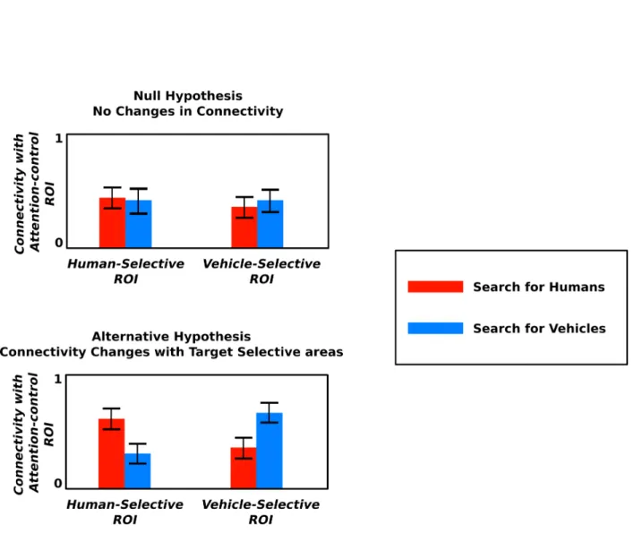
1.1 Null and alternative hypotheses. The null hypothesis suggests no atten-tional changes in connectivity between category-selective and attention-control ROIs, on the other hand, the alternative hypothesis suggests that attending to vehicle increases connectivity strength between areas selective for in-animate objects and attention-control areas, and attending to humans increases connectivity strength between areas selective for animate categories and attention-control areas. . . 3

2.1 Cerebral cortex in the human brain (modified from [1]). Cerebral cortex is divided into four lobes. . . 6

2.2 Flattened representation of the left hemisphere of the human brain showing various regions mentioned in Table 2.1. Areas selective for animate objects are shown by red boundaries, areas selective for in-animate objects by blue boundaries and the attention-control areas by green boundaries. . . 9

2.3 Hemodynamic response function (HRF). Initially there is a drop in the BOLD signal (0-2 s) after the stimulus is briefly displayed, then the signal rises and reaches its peak (5 s). An undershoot occurs after the peak and it takes some time for the signal to stabilize. . . 12

3.1 Experimental design. Subjects were shown three sets of movies twice, and were instructed to search for humans and vehicles in distinct runs. . . 13

(9)

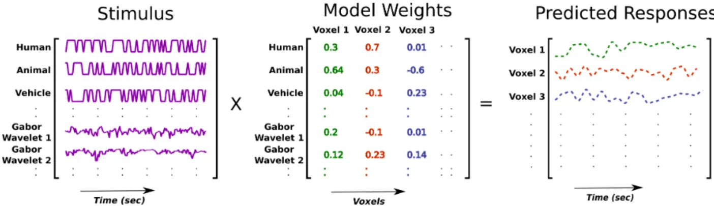
3.2 Estimation of predicted responses. Using L2-regularized regression, model weights were obtained. The model weights were then multiplied with the stimulus matrix to obtain the predicted responses. . . 19

3.3 Estimation of background responses. Background responses are generally ob-tained by subtracting the predicted responses from the raw BOLD responses. 20

3.4 To validate model performance, time course of stimulus and voxel responses were first divided into small chunks (50 time units each). Whole time series was then randomly split into 10 training (90%) and validation sets (10%). . . 22

3.5 Bootstrap sampling. In bootstrap sampling, sampling is done with re-placement, meaning that each re-sample can contain one observation multiple times. . . 27

3.6 Bootstrap hypothesis testing. Using the value of test-statistic under the null hypothesis (i.e. 0) p-value is obtained by dividing percentage of samples on the left side of the zero point on the x-axis (i.e. 0.9%) by 100. Here, for p-value threshold equal to 0.05 or 0.01, the null hypothesis can be rejected. However, it can not be rejected for p-value threshold equal to 0.001. . . 27

4.1 Attentional changes in inter-regional coherence (coherence during human search - coherence during vehicle search). Red blocks represent stronger con-nectivity during human search and blue blocks represent stronger concon-nectivity during vehicle search. The category-selective areas increased their connectiv-ity with attention-control areas based on the target category, and these pat-terns of connectivity were widely distributed. In addition to FFA and EBA, pSTS that is involved in processing human facial expressions, also increased its connectivity strength with attention-control ROIs while searching for humans. In addition, MT and LOC showed connectivity behaviours similar to the areas selective for human faces and body parts. All areas selective for scenes (PPA, RSC, and TOS) increased their connectivity with attention-control areas dur-ing vehicle search. . . 30

(10)

4.2 Attentional changes in inter-regional coherence in the background responses (coherence during human search - coherence during vehicle search). Red blocks represent stronger connectivity during human search and blue blocks represent stronger connectivity during vehicle search. The connectivity pat-terns observed between attention-control and category-selective regions were generally similar to those observed in the raw BOLD responses. However, there were several differences in the background connectivity analyses. The connectivity strength between SEF and areas selective for human faces and body parts was not stronger while searching for humans. Furthermore, the attentional changes in connectivity were not observed between EBA and FO. In addition, pSTS, MT, and LOC did not show any increase in connectivity strength with the attention-control areas during human search. All the areas selective for the scenes (PPA, RSC, and TOS) increased their connectivity with the attention-control areas during vehicle search. . . 32

4.3 Attentional changes in causality (causality during human search - causality during vehicle search). Red arrows represent stronger influence of attention-control areas on category selective areas during human search and blue arrows represent stronger influence during of attention-control areas on category se-lective areas during vehicle search. Numbers on the arrows represent the magnitude of the attentional changes in influence. These changes lie in the range [0,1]. Attentional changes in influence were observed in a few pairs of ROIs and unlike attentional changes in functional connectivity, they were not widely distributed. . . 33

4.4 Average correlation coefficient for a tested range of regularization parame-ters. Using 10-fold cross validation, optimum regularization parameter was estimated for each voxel separately for both attention conditions and it was averaged across the voxels. . . 37

4.5 Histogram showing average prediction scores (pearson correlation coefficient) for all five subjects. The x-axis shows the prediction scores, and the y-axis shows the number of voxels. . . 38

(11)

4.6 Prediction scores (mean Pearson correlation coefficient ± standard error) in functional regions averaged across subjects. Average correlation coefficients in all ROIs were greater than zero. However, the areas selective for animate objects (FFA and EBA) had higher prediction scores as compared to the areas selective for in-animate objects (PPA, RSC, and TOS) and the attention-control areas (IPS, FEF, SEF, and FO). SEF along with TPJ and PrC showed the lowest prediction scores. . . 39

4.7 Brain regions showing inverse connectivity patterns with category-selective regions (shown by purple boundaries). To investigate how the connectivity strength of category-selective areas changes with the rest of the voxels cover-ing the cortical surface, first principal component of multivariate time series of each category-selective area was obtained. Then principal component of the time series of each ROI was correlated with the time course of each in-dividual voxel of the cortical surface for both attention conditions and their difference was computed across the attention conditions. PCC (posterior cin-gulate gyrus) and vmPFC (ventro medial prefrontal cortex), shown by purple boundaries, showed reverse connectivity patterns with the category-selective areas, i.e., searching for a category decreased the connectivity strength of these areas with the target category-selective areas. . . 42

A.1 Attentional changes in connectivity of areas selective for animate objects with each individual voxel of the cortical surface for subject S1. Red color repre-sents stronger connectivity during human search and blue color reprerepre-sents stronger connectivity during vehicle search. . . 51

A.2 Attentional changes in connectivity of areas selective for in-animate objects with each individual voxel of the cortical surface for subject S1. Red color rep-resents stronger connectivity during human search and blue color reprep-resents stronger connectivity during vehicle search. . . 52

(12)

(13)

(14)

List of Tables

1.1 Attention-control and category-selective regions . . . 4

(15)

Chapter 1 Introduction

Every day we find ourselves searching for various objects. We look for a cab in a street or our friend in a crowded place. Given the complexity of natural scenes and the fact that human brain has limited resources for visual information processing [2], human brain shows remarkable capability to search for target objects in surrounding environment. It is thought that this capability is mediated by attention, a neural control mechanism that reallocates available brain resources to enhance performance during visual search tasks [2].

How does attention work and what are the underlying neural mechanisms of object-based attention? Human brain comprises separate category-selective regions in the anterior vi-sual cortex, specialized for the processing of ecologically important categories of objects like faces and body parts [3]. Furthermore, the dorsal part of frontal and parietal cortex form a network of regions implicated in attentional control [4]. It is assumed that attending to an object category modulates the activity in category-selective regions to enhance the rep-resentation of the attended category. These modulations are in the form of increased firing rate of neurons, and the frontoparietal attention network is believed to be the source of these modulations [4]. Several studies have reported attention-dependent interactions be-tween goal-relevant brain regions during object-based visual attention tasks [5, 6, 7]. In one study, it was reported that inferior frontal junction (IFJ) exerted stronger influence on a well-known face-selective region (fusiform face area (FFA)) while attending to faces, and increased its influence on a scene-selective area (parahippocampal place area (PPA)) while

(16)

area V4 and category-selective areas (PPA, FFA) was dependent on the attended object [8]. These studies were restricted to a small set of brain regions and focused on a small set of objects presented at fixed locations against a blank background. However, a recent study showed that attending to a category while watching natural movies alters the representa-tion of visual informarepresenta-tion throughout the human brain [9]. Furthermore, several animate and in-animate objects have been shown to have distributed representations throughout the anterior visual cortex (Table 1.1) [10, 11]. Therefore, it is more likely that attention alters connectivity patterns between category selective and attention control regions in the brain in a widely distributed fashion.

Are the inter-regional interactions during real-world visual search also widespread across the brain or only a small set of regions are involved as reported by the previous studies? To an-swer this question, we used an experimental design in which subjects watched natural movies while searching for either humans or vehicles. Their brain activity was recorded using func-tional magnetic resonance imaging (fMRI). Vehicles and humans were used because of their frequent appearance in daily life. If widespread inter-regional interactions exist, then at-tending to humans should increase connectivity strength between areas selective for animate objects and attention-control areas, and attending to vehicles should increase connectivity between areas selective for in-animate objects and attention-control areas (Fig 1.1).

To investigate the attentional effects on inter-regional coupling strength, we used coherence analysis [12]. As coherence provides no information about causal interactions, to examine the strength of the influence that attention-control regions exert on category-selective regions, Granger causality analysis was implemented [13].

Connectivity patterns observed by applying aforementioned analyses can be due to modula-tion of activity in different brain regions caused by visual stimuli appearing in the movies. To examine if there are any changes in connectivity after accounting for brain responses evoked by stimuli, the stimulus-evoked responses were regressed out using L2-regularized linear regression and the connectivity analyses were repeated on residuals.

To find out how connectivity strength of category-selective regions changes with the rest of the voxels covering the whole cortical surface, correlation was computed between time series of category-selective regions and each individual voxel of the cortical surface separately for both attention conditions. Then, the difference in connectivity measures between attention conditions was computed.

(17)

Figure 1.1: Null and alternative hypotheses. The null hypothesis suggests no attentional changes in connectivity between category-selective and attention-control ROIs, on the other hand, the alternative hypothesis suggests that attending to vehicle increases connectivity strength between areas selective for in-animate objects and attention-control areas, and attending to humans increases connectivity strength between areas selective for animate categories and attention-control areas.

(18)

Attention-control areas IPS (intraparietal sulcus)

FEF (frontal eye fields) SEF (supplementary eye fields)

FO (frontal operculum)

Areas selective for in-animate object categories Areas selective for animate object categories PPA (parahippocampal place area)

FFA (fusiform face area) RSC (restrosplenial cortex)

EBA (extrastriate body area) TOS (transverse occipital sulcus)

Table 1.1: Attention-control and category-selective regions

and attention-control network alters during visual search for two distinct objects. Chapter 2 includes some background information about the human brain, visual attention and fMRI. Chapter 3 focuses on the methods used for the connectivity analyses, model fitting and ex-perimental procedures. Chapter 4 goes through the key results obtained. The final chapter concludes this work and discusses potential future work.

(19)

Chapter 2 Background

2.1 The Human Brain

The brain is the most important part of the central nervous system. It controls our ability to perform daily life functions. Human brain makes up 2% of the total body’s mass, but uses 20% of the total energy, and consists of 86 billion neurons [14, 15]. From an evolutionary perspective, the cerebral cortex is the most advanced part of human brain. It is involved in higher order functions like thinking, memory, and attention. Cerebral cortex is divided into two hemispheres and each of them consists of four lobes (Fig 2.1) [16].

• Occipital Lobe : Occipital lobe is located at the back side of the brain. It is mainly involved in the visual information processing [17].

• Parietal Lobe : Parietal lobe is located above the occipital lobe. Its main functions include receiving and processing sensory information like touch, pressure, heat, and cold. It is also involved in the visuospatial processing, which helps us in representing the world around us by creating a spatial coordinate system [17].

• Temporal Lobe : It is located anterior to the occipital lobe and below the parietal lobe. It is primarily responsible for emotion, language, and memory [17].

(20)

Figure 2.1: Cerebral cortex in the human brain (modified from [1]). Cerebral cortex is divided into four lobes.

• Frontal Lobe : Frontal lobe is the frontal part of the hemisphere located in front of the parietal lobe and its functions include planning, thinking, reasoning, and attention [17].

2.2 Visual Processing

Light entering the eyes first hits the retina which is located at the back of the eyeball. The retina contains two types of cells called rods and cones. These photoreceptor cells convert light signals into neural signals. These signals are then passed on to the optic nerves. These nerves carry signals from both eyes and cross at a point called optic chiasm which is located at the bottom of the brain. At this crossing point neural signals get mixed and then split in such a way that the visual information from the right side of the visual field is directed to the left hemisphere, and the visual information from the left side of the visual field is directed to the right hemisphere. Information from optic nerves is passed onto lateral geniculate nucleus (LGN), and is eventually sent to the visual cortex of human brain. Visual stream in the

(21)

brain is hierarchically organized, with early visual areas representing low level features like edges and orientations, and as the information moves along, regions start showing selectivity for complex objects and features like faces and objects [18]. The visual stream is further subdivided into dorsal and ventral streams. Dorsal stream, also known as the ‘where’ stream, is involved in determining the positions of objects, while ventral stream, which is also known as the ‘what’ stream, is involved in identifying object categories [19].

2.3 Brain ROIs (Regions of Interest)

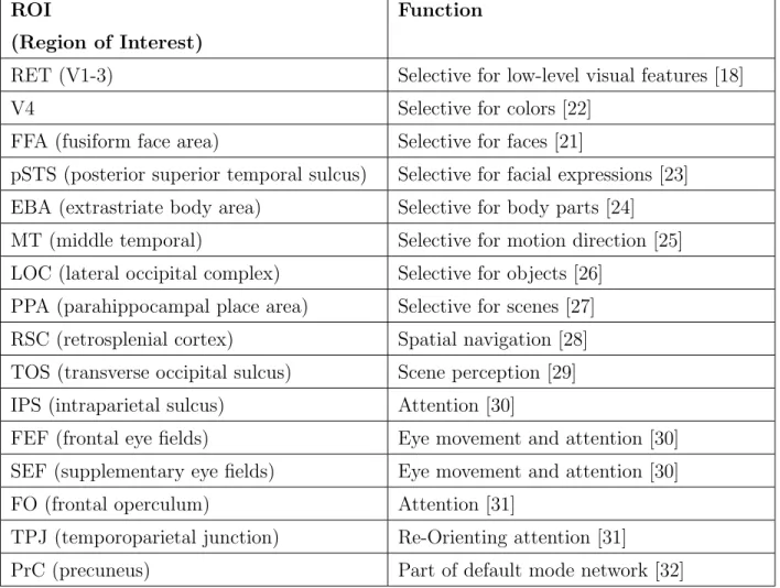
Human brain contains various regions that are defined based on their functions or anatomical locations (Fig 2.2). Some functional regions show selectivity for specific types of visual stim-uli like faces and objects, and others are involved in performing distinct tasks like attention and memory. Table 2.1 shows functions of ROIs in the human brain used in our analyses. The functional regions are localized by selecting voxels that show activation during that specific task or presence of a visual stimulus [20]. For example, fusiform face area (FFA) is a region in the brain that is selective for faces [21]. To localize FFA, human subjects are shown images of faces and familiar objects like spoon, car, or telephone, and their brain responses are recorded using functional magnetic resonance imaging (fMRI). Voxels showing significantly greater responses to faces as compared to objects are labelled as the voxels comprising FFA.

(22)

ROI Function (Region of Interest)

RET (V1-3) Selective for low-level visual features [18]

V4 Selective for colors [22]

FFA (fusiform face area) Selective for faces [21]

pSTS (posterior superior temporal sulcus) Selective for facial expressions [23] EBA (extrastriate body area) Selective for body parts [24] MT (middle temporal) Selective for motion direction [25] LOC (lateral occipital complex) Selective for objects [26]

PPA (parahippocampal place area) Selective for scenes [27] RSC (retrosplenial cortex) Spatial navigation [28] TOS (transverse occipital sulcus) Scene perception [29] IPS (intraparietal sulcus) Attention [30]

FEF (frontal eye fields) Eye movement and attention [30] SEF (supplementary eye fields) Eye movement and attention [30] FO (frontal operculum) Attention [31]

TPJ (temporoparietal junction) Re-Orienting attention [31]

PrC (precuneus) Part of default mode network [32]

Table 2.1: Functions of different ROIs in the human brain

2.4 Visual Attention

We come across thousands of complex objects in our daily lives. However, our brain has limited capacity for information processing. Visual attention refers to allocating limited brain resources by selecting behaviourally-relevant information and discarding unnecessary and irrelevant information. Based on our goals, attention can be allocated to spatial locations, visual features or objects.

(23)

Figure 2.2: Flattened representation of the left hemisphere of the human brain showing various regions mentioned in Table 2.1. Areas selective for animate objects are shown by red boundaries, areas selective for in-animate objects by blue boundaries and the attention-control areas by green boundaries.

(24)

or space in our visual field. By allocating attention to a location, we prioritize the information processing of that area in the visual field. For example, while playing football a defender might be attending to a specific location in his visual field to keep a check on other team’s players.

• Feature-based attention : In feature-based attention, we attend to features like colors and shapes. For example, if we want to look for a person wearing a green shirt, we would search for people wearing green coloured shirts.

• Object-based attention : In object-based attention, the attention is allocated to an object category like faces, animals, and cars. For example, while playing tennis, the players would continuously attend to the ball.

2.5 Brain Connectivity

Brain connectivity refers to anatomical connections or mutual dependence between different units in the brain. A unit can be an individual neuron or a population of neurons. In this work, brain units refer to ROIs used in the analyses. Interactions between different units can occur because of physical links like synapses or fibres, or because of mutual dependence or causal interactions. These interactions can occur while preforming a task or even when we are not performing any explicit task. Neuronal interactions can be categorized into three different types.

• Structural Connectivity : Structural connectivity refers to the presence of anatom-ical connections between brain units. These connections can occur via synapses, which are connections through which information flows from one neuron to another or they can also occur through white nerve fibres present in the brain.

• Functional Connectivity : Functional connectivity is defined as the existence of mutual dependence between spatially segregated brain units. It tells us about the association between the time series of different brain units. It does not give us any information about causal effects, nor does it use any information about the underlying anatomical connections. It uses the idea that if two units share similar functionalities

(25)

during a task, then their time series will be highly correlated. Correlation and coherence analyses are the measures generally used to infer functional connectivity [33].

• Effective Connectivity : Effective connectivity describes the causal effect of one neu-ral system over the other. Mostly, the methods used to infer effective connectivity take into account both anatomical architecture and time series of brain units. DCM (dy-namic causal modelling), SEM (structure equation modelling), and Granger causality analysis are the most commonly used methods to infer effective connectivity [33].

2.6 Functional Magnetic Resonance Imaging (fMRI)

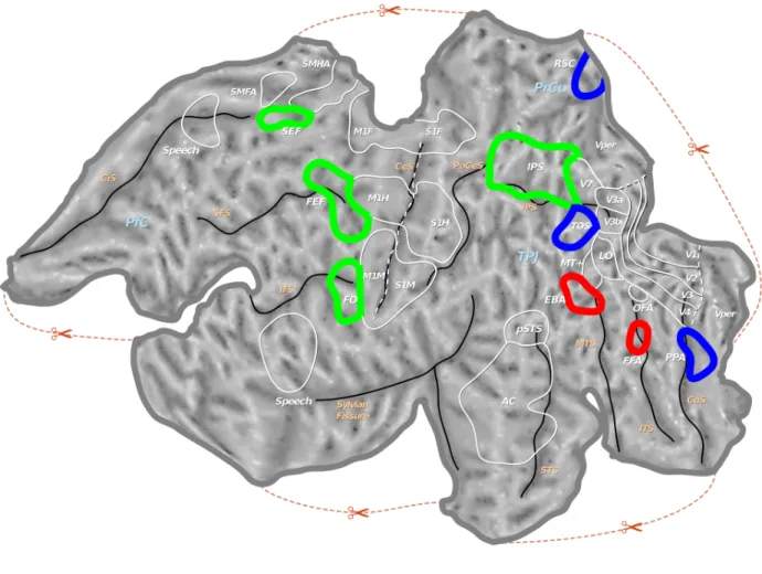
Functional magnetic resonance imaging (fMRI) is a non-invasive imaging technique used to measure brain activity. fMRI does not measure brain activity directly, instead it measures the physiological changes that are caused by neuronal activation [34]. Activation of neurons in our brain causes increase in metabolic requirements. To meet these demands, the circulatory system provides energy in the form of glucose and oxygen. This causes an increase in oxygenated blood flow. Oxygen is delivered to neurons via hemoglobin. Oxygenated and de-oxygenated hemoglobin have different magnetic properties which cause changes in measured MR signal. This variation in signal caused by change in oxygen level is called blood-oxygen-level dependent (BOLD) effect, which can be used to infer brain activity.

The change in MR signal caused by neuronal activity is referred to as the hemodynamic response function. Neuronal responses occur tens of milliseconds after the stimulus onset. However, it takes 1-2 s for the hemodynamic responses to start changing. Initially, the consumption of oxygen by neurons leads to an increase in the amount of deoxyhemoglobin. Therefore, an initial dip in MR signal is observed as shown in Fig 2.3. The signal starts increasing 2 s after the stimulus onset and reaches a peak point after approximately 5 s. If the activation of the neuronal population is prolonged, the peak is maintained, however, it is slightly lower than the peak point. When the neuronal activity ceases, an undershoot occurs. This undershoot is generally explained by the balloon model [34].

According to this model, when neurons get activated the blood inflow increases. Blood inflow is greater than the outflow, therefore, the venous system swells like a balloon. When the neuronal activity ceases, the blood flow decreases more rapidly as compared to the blood

(26)

Figure 2.3: Hemodynamic response function (HRF). Initially there is a drop in the BOLD signal (0-2 s) after the stimulus is briefly displayed, then the signal rises and reaches its peak (5 s). An undershoot occurs after the peak and it takes some time for the signal to stabilize.

volume. As the blood flow goes back to the normal rate quickly and the volume remains expanded, this increases the amount of deoxyhemoglobin and causes a decrease in MR signal. Henceforth, an undershoot is observed. The signal goes back to its baseline state as the blood volume returns to its normal state.

fMRI measures the BOLD signal in small rectangular units called voxels. In the experimental design used, voxels were 2x2x4 mm3 in size, and approximately 30,000 voxels were covering the surface of the cerebral cortex.

(27)

Chapter 3 Experimental Setup and Methods

3.1 Experimental Setup

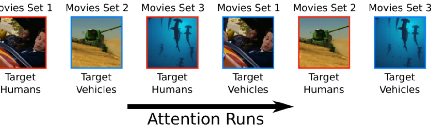
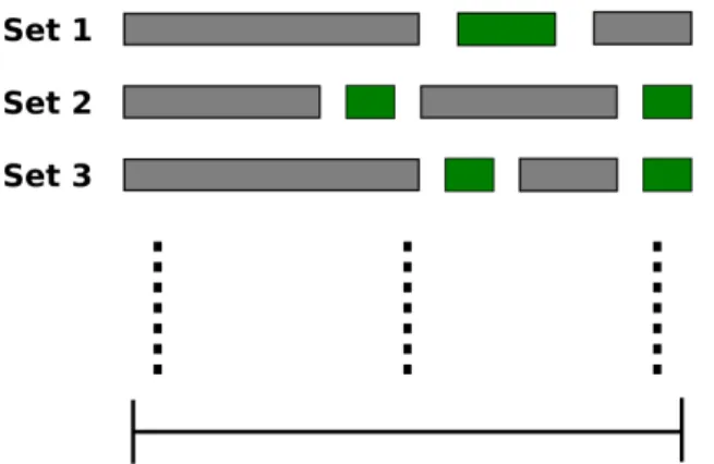
MRI data were acquired from five human subjects with a sampling rate of 0.5 Hz. The subjects were shown two hours of identical natural movies twice (Fig 3.1). The subjects were instructed to search for humans or vehicles while maintaining their visual gaze at a fixation point, which was appearing at the center of the visual field. Furthermore, to ensure their behavioural performance, the subjects were given a button response pad and they were told to press the button every time they detected a target.

Figure 3.1: Experimental design. Subjects were shown three sets of movies twice, and were instructed to search for humans and vehicles in distinct runs.

(28)

• Stimulus - During each attention session subjects were shown 1800 s long natural movies. These movies were made by compiling 10-20 s short clips without any rep-etition. These movies were structured in such a way that four categories of stimuli (humans, vehicles, both humans and vehicles, none of them) appeared in an evenly distributed manner. Each category of stimulus appeared for 450 s. A fixation point was overlaid on the center of the visual field. Its color was altered every 1 s to make sure that it remains visible throughout the movies.

• Stimulus Labeling - 604 object and action categories appearing in the movies were labelled by three raters, using words from Wordnet database. Wordnet consists of hierarchical organization of object and action categories such that words with similar meaning are closer in proximity to each other [35]. Using Wordnet lexicon, additional 331 super ordinate categories were inferred, for example, the presence of a ‘cat’ indi-cated the presence of superordinate categories like ‘mammal’, and ‘vertebrate’. Using this labelling, a stimulus matrix indicating presence or absence of a category during each 1 s clip was formed. Presence of a category was denoted by 1 and absence was denoted by 0. This stimulus matrix was down-sampled to match the sampling rate of responses.

3.2 Methods

This section explains the methods used in the analyses in detail. To infer the attentional effects on the connectivity strength between pairs of brain regions, coherence analysis was implemented. Section 3.2.1 explains the coherence analysis. However, coherence is a non-directional measure of association. Therefore, to examine the attentional effects on the influence of the attention-control regions on the category-selective regions, Granger causal-ity analysis was employed. Section 3.2.2 covers the Granger causalcausal-ity analysis.

First, coherence and Granger causality analyses were carried out on raw BOLD responses. To investigate if the attention-dependent connectivity patterns still persist even after remov-ing stimulus-driven brain activity, L2-regularized linear regression was used to predict the stimulus-evoked responses in each individual voxel separately. These predicted responses were projected out of the raw fMRI responses to obtain the background responses, and the

(29)

connectivity analyses were repeated on these background responses. Section 3.2.3 illustrates methods used to obtain the background responses.

Furthermore, to examine the attentional changes in connectivity of category-selective areas with the rest of the voxels covering the whole cortical surface, the time series of category-selective regions was correlated with each individual voxel of the cortical surface separately. The voxel-level connectivity analysis is further explained in Section 3.2.4.

Coherence is a bi-variate measure of association, however the responses of brain regions were in the form of multivariate time series. Therefore, principal component analysis was used to reduce the dimension of multivariate time series of ROIs to univariate time series. Sec-tion 3.2.4 explains the principal component analysis used for dimensionality reducSec-tion. To investigate whether the attentional changes in connectivity between pairs of brain regions were significant or not, bootstrap significance test was performed. Section 3.2.5 describes the bootstrap method used for hypothesis testing.

3.2.1 Coherence Analysis

To measure coupling strength between pairs of brain regions, coherence analysis was em-ployed. Coherence is normalized cross-covariance in frequency domain [12]. Coherence gives a value in the range [0, 1], 0 implying incoherent and 1 implying fully coherent signals. Mean of coherence across a specific frequency band gives a measure of inter-regional connectivity. Coherence between activities of two ROIS, X and Y is given as:

CohXY(f ) =

|GXY(f )| 2

GXX(f )GY Y(f )

, (3.1)

where GXY(f ) is the cross-spectral density between time series of ROIs X and Y , GXX(f )

and GY Y(f ) are auto-spectral densities of X and Y , and f is the frequency. Auto-spectral

density is obtained by computing the Fourier transform of auto-covariance function, or mul-tiplying Fourier transform of one time series with the conjugate of its Fourier transform. Cross-spectral density is obtained by computing Fourier transform of the cross-covariance function between the time series of two ROIs, or multiplying the Fourier transform of one time series with the conjugate of the Fourier transform of the other time series.

(30)

The hemodynamic response shape can differ from region to region [36]. As coherence de-scribes similarity in frequency domain, it is invariant to shape differences in hemodynamic responses of different voxels [12].

Welch’s Periodogram

For coherence estimation Welch’s method was employed [37]. In Welch’s method, response time course of each ROI is divided into overlapping segments of time by using a windowing function. All time segments are then projected into the frequency domain by calculating their Fourier transform. Subsequently, auto-spectral and cross-spectral densities are obtained for each segment and their mean is computed across the segments. Mean of auto-spectral and cross-spectral densities across segments are then used to calculate coherence between complete time series of two ROIs. Estimated coherence is given as:

ˆ CohXY(f ) = GˆXY(f ) 2 ˆ GXX(f ) ˆGY Y(f ) , (3.2)

where ˆCohXY(f ) is the estimated coherence and:

ˆ GXY(f ) = 1 N N X k=1 Xk(f )Yk∗(f ), (3.3) ˆ GXX(f ) = 1 N N X k=1 Xk(f )Xk∗(f ), (3.4) ˆ GY Y(f ) = 1 N N X k=1 Yk(f )Yk∗(f ), (3.5)

where k represents the windowed segment, N represents the total number of segments, X(f ) and Y (f ) represent the Fourier transforms of X and Y, and X∗(f ) and Y∗(f ) represent conjugates of Fourier transforms of X and Y. For coherence estimation, Hanning windows with size of 60 times units and 50% overlap were used, as these values give a good estimate of coherence [12].

The hemodynamic response function acts as a low pass filter [38]. Therefore, generally overall coherence is reported by taking mean of coherence between 0-0.15 Hz [12]. However, instead

(31)

of limiting the analysis to a specific frequency band, here weighted coherence was employed using complete frequency range (0-0.25 Hz).

Weighted Coherence

Weighted coherence gives information about the activity of ROI X shared with ROI Y, within the dominant frequency range of activity of both ROIs. Weighted coherence between time series of two ROIs is obtained by first weighting the coherence at all frequencies by auto spectral density of the time series of both ROIs separately [39].

Weighting by GXX we get: CohwX = f 2 R f 1 CohXY(f )GXX(f )df f 2 R f 1 GXX(f )df . (3.6) Weighing by GY Y we get: CohwY = f 2 R f 1 CohXY(f )GY Y(f )df f 2 R f 1 GY Y(f )df . (3.7)

Then they are averaged to obtain overall weighted coherence.

Cohw =

CohwX + CohwY

2 , (3.8)

where Cohw is the average weighted coherence between the time series of two ROIs, X and

Y.

3.2.2 Granger Causality

To investigate attentional changes in the influence of attention-control areas on category-selective areas, Granger causality was implemented [13]. Granger causality is a technique

(32)

the past of Y along with X is a better predictor of past of X as compared to X alone. To infer causality, the present values of X are first predicted using an autoregressive model. In the autoregressive model, the present values of a variable are predicted using a linear combination of its past values.

X(t) =

p

X

k=1

A0_xx(k).X(t − k) + ε0_x(t), (3.9)

where A0_xx represents the regression coefficients when the past k values of X are used to predict its present values and ε0_x represents the residuals.

Afterwards, to predict the present values of X using both X and Y, the past values of Y are added as regressors to the autoregressive model.

X(t) = p X k=1 Axx(k).X(t − k) + p X k=1 Axy(k).Y (t − k) + εx(t), (3.10)

where Axy represent the regression coefficients when k past values of Y are used to predict

the present values of X, and εxrepresents the residuals. Influence of Y on X can be obtained

using Granger causality index (GCI), which is given as:

GCIY →X = 1 − ln

var(εx(t))

var(ε0 x(t))

. (3.11)

In a similar way GCIX→Y can be obtained. GCI lies in the range [0,1]. As Granger causality

is obtained by computing ln ratio of var(εx(t)) and var(ε0x(t)), increasing the value of k

always decreases this ratio. However, after a certain value of k, the model starts overfitting. To avoid overfitting, a criterion is needed that can penalize the number of model parameters. For this purpose, Bayesian information criterion (BIC) was used [40]. BIC is given by:

BIC = −2 ln ˆL + k. ln(n), (3.12)

where ˆL is the likelihood obtained by fitting present values of both X and Y using their past values, k is the number of model parameters or the number of previous time points, and n is the total number of time points. The likelihood function is defined as:

ˆ L = 1 n n X t=1 (Z(t) −Z(t))ˆ 2, (3.13)

where Z(t) represents the original time series of pair of regions for which we are trying to estimate k, and Z(t) represents fitted values by using linear regression. Linear regression isˆ

(33)

Figure 3.2: Estimation of predicted responses. Using L2-regularized regression, model weights were obtained. The model weights were then multiplied with the stimulus matrix to obtain the predicted responses.

mentioned in Section 3.2.3.2 in detail. As BIC is directly proportional to the log likelihood function and the number of parameters used to construct the model, the model with the lowest value of BIC was chosen for causality estimation.

3.2.3 Background Connectivity

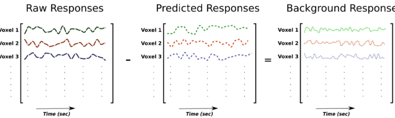
Normally the connectivity analyses are performed on the raw BOLD responses. However, the attentional changes in connectivity observed by applying aforementioned analyses on the raw fMRI responses can be due to modulation of activity in the brain regions caused by visual stimuli appearing in the movies. To examine if there are any changes in connectivity after accounting for brain responses evoked by the visual stimuli, a recently developed approach called background connectivity analysis was used [8, 41]. In the background connectivity analysis, the stimulus-dependent responses are first predicted by linearly fitting the model that best describes the voxel responses (Fig 3.2). These predicted responses are then sub-tracted from the raw fMRI responses to obtain stimulus-independent responses (Fig 3.3). These stimulus-independent responses are referred to as the background responses.

Yraw = Ypred+ Yback, (3.14)

where Yraw, Ypred, and Yback are raw, predicted, and background responses respectively.

(34)

Figure 3.3: Estimation of background responses. Background responses are generally ob-tained by subtracting the predicted responses from the raw BOLD responses.

3.2.3.1 Model Fitting

To obtain predicted responses, a voxel-wise model was fit using L2-regularized linear regres-sion. In model fitting, we try to find out how well the dependent variables can be explained by the independent variables. These independent variables are also called as regressors. Two types of regressors were used. The first type of regressors denoted object (humans, vehicles, etc.) and action (flying, diving, etc.) categories appearing in the movies, and the second type characterized the motion energy of the movies at each time instant. The regressors denoting object and action categories were used to explain the activity in the higher visual and non-visual areas of the brain. The regressors characterizing motion energy were obtained by passing visual stimuli at every time instant through 2139 Gabor filters having different positions, directions, shapes, and spatial and temporal frequencies [42]. Early visual areas in the human brain (V1-4) are involved in processing structural properties of scenes (like orientation and motion direction). Therefore, these regressors were added to predict the activity of early visual areas in the brain due to the low-level visual features.

All categories were labelled every 1 s in the movie. Therefore, to match the time courses of the stimuli with the sampling rate of responses (2 s), the time courses of the stimuli were temporally down sampled by averaging every two consecutive samples. After stimulus onset it takes some time for BOLD signal to reach its peak point, therefore, to compensate for hemodynamic lag, we replaced each regressor by 3 regressors representing the original one delayed by 2, 4 and 6 s. Model fitting was done separately for both attention conditions.

(35)

3.2.3.2 Linear Regression

Linear regression is a technique that is used to fit a model by finding a linear relationship between dependent variable Y and independent variable X.

Y = XW + ε, (3.15)

where X represents the stimulus matrix, Y represents voxel responses, W are the model weights that describe the relationship between X and Y , and ε are the errors or residuals. Model weights are generally obtained using the least squares approach. In this approach, sum of square of the residuals is minimized by minimizing the derivative with respect to the model weights.

J (W ) = (Y − XW )T(Y − XW ), (3.16) where J (W ) is the cost function. Minimizing the derivative with respect to model weights, we obtain:

W = (XTX)−1XTY. (3.17) However, using a large number of regressors can lead to overfitting. Overfitting means that the model performs well on the training data, but performs poorly on the test data. To avoid overfitting, L2-regularized regression was used. In L2-regularized regression, we penalize the model weights with a penalty term λ. So, the cost function becomes:

J (W ) = (Y − XW )T(Y − XW ) + λWTW. (3.18)

Minimizing the derivative with respect to model weights, we obtain:

W = (XTX + λI)−1XTY. (3.19)

3.2.3.3 Regularization Parameter Selection and Model Validation

Data were first randomly split into a training set (90%) and an independent validation set (10%) (Fig 3.4). k-fold cross validation was then applied to the training set to obtain prediction scores for a wide range of regularization parameters (24 − 218_{). In k-fold cross}

(36)

the chunks are used for testing once. First, we applied 10 fold-cross validation. Then mean of prediction scores was computed across folds to obtain average prediction scores for all regularization parameters. This whole procedure was repeated for each training set and the prediction scores were averaged across the training sets. For each voxel, the regularization parameter showing the highest average prediction score was used to obtain model weights for each training set. These model weights were used to predict the responses of the validation sets and the predicted responses were compared with the actual responses to get the mean prediction scores across all validation sets. Voxel-wise model was fit separately for both attention conditions. Therefore, to get prediction scores of voxels across both conditions, models weights were first estimated separately for both attention conditions. These model weights were then used to predict responses of the validation data. Finally, these predicted responses were then compared with actual responses and they were averaged across attention conditions to get overall prediction scores.

Figure 3.4: To validate model performance, time course of stimulus and voxel responses were first divided into small chunks (50 time units each). Whole time series was then randomly split into 10 training (90%) and validation sets (10%).

After obtaining optimum regularization parameters for all the voxels, the complete time course of responses and stimuli was used to estimate model weights and Ypred was obtained

(37)

by multiplying the stimulus matrix with the model weights.

Ypred = XW. (3.20)

3.2.3.4 Measure of Prediction Scores

Pearson correlation coefficient was used as a measure of the prediction scores. Pearson cor-relation coefficient measures the normalized linear corcor-relation between two variables, giving a value in the range [-1,1]. Here, 1 denotes total correlation, 0 mean no correlation, and -1 implies negative correlation. Pearson correlation coefficient between two variables x and y is defined as: r = Pn k=1(xk− x)(yk− y) q Pn k=1(xk− x) q Pn k=1(yk− y) , (3.21)

where r is the Pearson’s correlation coefficient between variables x and y with mean x and y, and n is the number of samples.

3.2.3.5 Background Responses Estimation

During model fitting, as the model weights were penalized heavily by using large regulariza-tion parameters, the variance of predicted responses was smaller as compared to the variance of the raw responses. Hence, instead of subtracting the predicted responses directly from the raw responses, the raw responses were first projected onto the predicted responses and then this projection was subtracted from the raw responses. First, the predicted responses were obtained as mentioned in the previous sections, and using principal component analysis, 1st principal component of each ROI was computed separately. Principal component anal-ysis is a technique used for dimensionality reduction, and it is further explained in Section 3.2.5. After that, for each ROI, 1st principal component of the raw responses was projected onto the 1st principal component of the predicted responses. Finally, this projection was subtracted from the raw responses to obtain the background responses.

(38)

where projYrawYpredis the projection of the raw BOLD responses onto the predicted responses.

This projection was removed from the raw BOLD responses to obtain the background re-sponses.

All connectivity analyses were carried out on visually responsive voxels, i.e., the voxels that were tuned for categories and low-level visual features used in the voxel-wise model fitting. Therefore, the voxels showing high prediction scores were used. For each ROI, the voxels showing high prediction scores were defined as the ones showing prediction scores greater than the average prediction scores of each ROI.

3.2.4 Voxel-Level Connectivity Analysis

To observe attentional changes in connectivity of category-selective ROIs with the rest of the voxels covering the whole cortical surface, first principal component of multivariate time-course of each category-selective ROI was obtained. It was then correlated with the response of each individual voxel of the cortical surface separately for both attention conditions. Their difference was then computed and projected onto a flattened representation of cortical surface. Pearson correlation coefficient was used as a measure of association.

Prior to this analysis, spatial smoothing was done on the responses of all the voxels of cortical surface. First, a voxel-neighbourhood of size 3x3x3 was formed around each voxel. Then, the mean response of all the voxels in the neighbourhood was assigned to the central voxel. Again, for the voxel-level connectivity analysis, the voxels in each category-selective area showing high prediction scores were used.

3.2.5 Principal Component Analysis

Activity in each ROI is represented by a multivariate time series. However, coherence is a bivariate measure of association. Therefore, to get univariate time series representing each ROI activation, the principal component analysis was implemented. Principal component analysis is a dimensionality reduction technique in which n features (voxels in our case) are projected onto a new feature space, in such a way that less number of features m can explain most of the data variance [43]. These new features are called the principal components. The

(39)

principal components are obtained by taking eigenvectors of the co-variance matrix of the matrix, containing responses of all the voxels. These eigenvectors are then multiplied with the response matrix to obtain a new set of features. As the eigenvectors are arranged in descending order of their eigenvalues, the first principal component explains the maximum variance of the data. The covariance matrix is given as:

C = Y

T roiYroi

n − 1 , (3.23)

where Yroiis the matrix containing responses of all the voxels in an ROI and n is the number

of time points. Using the singular value decomposition, it can be written as:

C = V SU

T_{U SV}T

n − 1 , (3.24)

where columns of U are left singular vectors, rows of V are right singular vectors, and S is the diagonal matrix containing the singular values obtained by computing the singular value decomposition of Yroi.

C = V S

2_VT

n − 1 , (3.25)

where S corresponds to diagonal matrix containing eigenvalues arranged in descending order and V contains eigenvectors of co-variance matrix.

Features in the new projected space are given as:

Y_roi0 = XV, Y_roi0 = U SV0V = U S,

where Y_roi0 is the matrix containing principal components of Yroi. First principal component

was used for each region in the brain, because it explains maximum variance of responses of all the voxels in each ROI.

3.2.6 Hypothesis Testing

To investigate whether the attentional changes in connectivity between pairs of brain regions were significant or not, they were passed through bootstrap significance test.

(40)

the hypothesis, samples are obtained from a population and they are statistically analysed. Based on statistical analysis, hypotheses are accepted or rejected.

• Null Hypothesis : Null hypothesis states that all sample observations are obtained by chance. It is generally denoted by Ho. Null hypothesis in this study was that

attention would not alter inter regional connectivity.

• Alternative Hypothesis : In contrast, alternative hypothesis states that sample observations are not random. It is generally denoted by Ha. Alternative hypothesis in

this study was that searching for a category would strengthen the connectivity between category-selective and attention-control ROIs.

• Test Statistic : Test statistic is a normalized value calculated from sample data to test the validity of the null hypothesis. Based on the test statistic, we can reject or accept the null hypothesis. In this study, the mean of difference in connectivity strength across subjects was used as a test statistic.

• p-value : p-value is defined as the probability of obtaining the observed test statistic further away from null distribution, given that null hypothesis is true. Generally, for hypothesis testing, a threshold is set for p-value. If the p-value is less than the threshold value, then the null hypothesis is rejected in favour of the alternative hypothesis. To investigate the significant changes in attention, the threshold for hypothesis testing was set to 0.05.

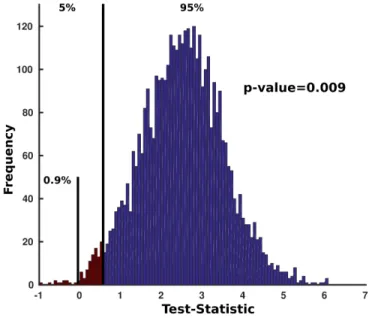
• Bootstrap Hypothesis Testing : Bootstrap is a statistical technique used for hy-pothesis testing. It is preferred over other statistical tests when sample size is small. It makes use of the bootstrap re-sampling method. Re-sampling means to produce artificial samples from the sample we already have. In bootstrap, re-sampling is done with replacement, meaning that each re-sample can contain one observation multiple times [44]. Fig 3.5 shows bootstrap re-sampling from a sample having four observations n1, n2, n3 and n4.

(41)

Figure 3.5: Bootstrap re-sampling. In bootstrap re-sampling, sampling is done with replace-ment, meaning that each re-sample can contain one observation multiple times.

Using the generated samples, we can obtain the distribution of our test-statistic, which along with the value of test-statistic under null distribution, can be used to calculate p-value. Based on the p-value threshold, the null-hypothesis can be accepted or rejected.

Figure 3.6: Bootstrap hypothesis testing. Using the value of test-statistic under the null hypothesis (i.e. 0) p-value is obtained by dividing percentage of samples on the left side of the zero point on the x-axis (i.e. 0.9%) by 100. Here, for p-value threshold equal to 0.05 or 0.01, the null hypothesis can be rejected. However, it can not be rejected for p-value

(42)

Fig 3.6 elaborates bootstrap hypothesis testing in detail with the help of an example. In this study, for each pair of ROIs, there were five observations for difference in connectivity strength. Therefore, 55 bootstrap samples were generated and the distribution of the sample mean was obtained. The null hypothesis was that attentional change in connectivity strength is 0. Based on this hypothesis, p-value was evaluated. Setting the p-value threshold equal to 0.05, connectivity changes between pairs of ROIs were labelled as significant or insignificant.

(43)

Chapter 4 Results

4.1 Results

4.1.1 Inter-Regional Connectivity in Raw BOLD Responses

Coherence analysis was performed for each attention condition separately, to examine the effects of attention on inter-regional connectivity patterns. For this purpose, the coher-ence strength was contrasted across the attention conditions. Fig 4.1a shows attentional changes in connectivity. As expected, the coherence between the areas selective for animate objects and the attention-control areas was greater while searching for humans, and the coherence between the areas selective for in-animate objects and the attention-control areas was greater while searching for vehicles. However, to see if these patterns were significant or not, they were passed through bootstrap significance test. Fig 4.1b shows significant changes in coherence (p<0.05). The category-selective areas increased their connectivity with attention-control areas based on the target category, and these patterns of connectivity were widely distributed. Furthermore, in addition to FFA and EBA, pSTS that is involved in processing human facial expressions, also increased its connectivity strength with attention-control ROIs while searching for humans. In addition, MT and LOC showed connectivity behaviours similar to the areas selective for human faces and body parts.

(44)

(a) All changes in connectivity

(b) Significant changes in connectivity obtained by setting p-value threshold equal to 0.05

Figure 4.1: Attentional changes in inter-regional coherence (coherence during human search - coherence during vehicle search). Red blocks represent stronger connectivity during human search and blue blocks represent stronger connectivity during vehicle search. The category-selective areas increased their connectivity with attention-control areas based on the target category, and these patterns of connectivity were widely distributed. In addition to FFA and EBA, pSTS that is involved in processing human facial expressions, also increased its con-nectivity strength with attention-control ROIs while searching for humans. In addition, MT and LOC showed connectivity behaviours similar to the areas selective for human faces and body parts. All areas selective for scenes (PPA, RSC, and TOS) increased their connectivity with attention-control areas during vehicle search.

(45)

All areas selective for scenes (PPA, RSC, and TOS) increased their connectivity with attention-control areas during vehicle search.

4.1.2 Inter-Regional Connectivity in Background Responses

To examine whether the connectivity patterns observed in raw responses still persist even after removing the effect of stimulus-evoked responses from raw responses, the coherence analysis was repeated on the background responses. Fig 4.2a shows attentional changes in connectivity in background responses and Fig 4.2b shows significant changes in connectiv-ity (p<0.05). The connectivconnectiv-ity patterns observed between attention-control and category-selective regions were generally similar to those observed in the raw BOLD responses. How-ever, there were several differences in the background connectivity analyses. The connectivity patterns between SEF and areas selective for human faces and body parts were not stronger while searching for humans. Furthermore, the attentional changes in connectivity were not observed between EBA and FO. In addition, pSTS, MT, and LOC did not show any increase in connectivity strength with the attention-control areas during human search.

All the areas selective for the scenes (PPA, RSC, and TOS) increased their connectivity with the attention-control areas during vehicle search. Overall, the results showed that at-tentional changes in connectivity were widespread, and were not just due to the modulation in the responses caused by the visual stimuli appearing.

(46)

(a) All changes in background connectivity

(b) Significant changes in connectivity obtained by setting p-value threshold equal to 0.05

Figure 4.2: Attentional changes in inter-regional coherence in the background responses (coherence during human search - coherence during vehicle search). Red blocks represent stronger connectivity during human search and blue blocks represent stronger connectivity during vehicle search. The connectivity patterns observed between attention-control and category-selective regions were generally similar to those observed in the raw BOLD re-sponses. However, there were several differences in the background connectivity analyses. The connectivity strength between SEF and areas selective for human faces and body parts was not stronger while searching for humans. Furthermore, the attentional changes in con-nectivity were not observed between EBA and FO. In addition, pSTS, MT, and LOC did not show any increase in connectivity strength with the attention-control areas during hu-man search. All the areas selective for the scenes (PPA, RSC, and TOS) increased their connectivity with the attention-control areas during vehicle search.

(47)

4.1.3 Causality

Coherence is an undirected measure of association. It provides no information about the influence of one neural system on the other. To examine the influence of attention-control areas on category-selective areas, the Granger causality analysis was employed. Granger causality measures how well the past values of a causing variable can explain the present values of the caused variable. To identify number of previous time units used in the analysis, Bayesian information criterion was used.

(a) Attentional changes in causality in raw BOLD responses

(b) Attentional changes in causality in background responses

Figure 4.3: Attentional changes in causality (causality during human search - causality during vehicle search). Red arrows represent stronger influence of attention-control areas on category selective areas during human search and blue arrows represent stronger influence during of attention-control areas on category selective areas during vehicle search. Numbers on the arrows represent the magnitude of the attentional changes in influence. These changes lie in the range [0,1]. Attentional changes in influence were observed in a few pairs of ROIs

(48)

Using the optimum number of previous time units obtained by using the BIC, the influence of the attention-control areas on the category-selective areas was estimated between pairs of ROIs that showed significant changes in coherence (as shown in Fig 4.1b and Fig 4.2b). Fig 4.3a shows significant (p<0.05) attentional changes in the influence of the attention-control areas on the category-selective areas in raw BOLD responses. Attentional changes in influence were observed in a few pairs of ROIs and unlike attentional changes in functional connectivity, they were not widely distributed. Similar analysis was repeated on the back-ground responses and the influence of the attention-control areas on the category-selective areas were contrasted across attention conditions. Fig 4.3b shows significant (p<0.05) atten-tional changes in the influence.This indicates that while performing visual search for a specific target category, the attention-control ROIs increase their influence on the category-selective ROIs.

4.1.4 Regularization Parameter Selection and Model Performance

Using 10-fold cross validation, the optimum regularization parameter was selected for each individual voxel separately for each attention condition. Fig 4.4 shows correlation coefficients averaged across all the voxels in an individual subject, for a tested range of regularization parameters. We observed that the mean correlation coefficient was maximum around 104₋

(49)

(a) Subject 1

(50)

(c) Subject 3

(51)

(e) Subject 5

Figure 4.4: Average correlation coefficient for a tested range of regularization parameters. Using 10-fold cross validation, optimum regularization parameter was estimated for each voxel separately for both attention conditions and it was averaged across the voxels.

Model performance was validated on 10% held out data as explained in Section 3.2.3. As this process was repeated 10 times separately, prediction scores were averaged across all the sets. Fig 4.5 shows mean prediction scores of all the voxels in the form of histograms. Fig 4.6 shows the prediction scores of ROIs used in the analysis averaged across subjects. Average correlation coefficients in all ROIs were greater than zero. However, the areas selective for animate objects (FFA and EBA) had higher prediction scores as compared to the areas selective for in-animate objects (PPA, RSC, and TOS) and the attention-control areas (IPS, FEF, SEF, and FO). SEF along with TPJ and PrC showed the lowest prediction scores.

(52)

(a) Subject 1 (b) Subject 2

(c) Subject 3 (d) Subject 4

(e) Subject 5

Figure 4.5: Histogram showing average prediction scores (pearson correlation coefficient) for all five subjects. The x-axis shows the prediction scores, and the y-axis shows the number of voxels.

(53)

Figure 4.6: Prediction scores (mean Pearson correlation coefficient ± standard error) in functional regions averaged across subjects. Average correlation coefficients in all ROIs were greater than zero. However, the areas selective for animate objects (FFA and EBA) had higher prediction scores as compared to the areas selective for in-animate objects (PPA, RSC, and TOS) and the attention-control areas (IPS, FEF, SEF, and FO). SEF along with TPJ and PrC showed the lowest prediction scores.

4.1.5 Voxel-Level Connectivity Analysis

To investigate how the connectivity of category-selective areas changes with the rest of the voxels covering the whole cortical surface, first principal component of multivariate time se-ries of each category-selective area was obtained. The first principal component of the time

(54)

series of each ROI was then correlated with each individual voxel of the cortical surface for both attention conditions. Their difference across the attention conditions was computed and projected onto a flattened representations of the cortical surface. Consistent with the results obtained from the coherence analysis, searching for a category increased the connec-tivity between the category-selective and the attention-control areas. However, in addition to the attention-control areas, some areas in the brain consistently showed reverse connec-tivity patterns with the category-selective areas, i.e., searching for a category decreased the connectivity strength of these areas with category-selective areas. These areas include PCC (posterior cingulate gyrus) and vmPFC (ventro medial prefrontal cortex), which are known to constitute DMN (default mode network). The DMN is a network of brain areas that increases its activity when the brain is not involved in any task, and decreases its activity during tasks. These effects were consistent across subjects and were observed in areas se-lective for both animate and in-animate objects. Fig 4.7 shows the regions showing inverse connectivity patterns with the category-selective areas.

For each subject, attentional changes of the category-selective areas with the whole cortical surface are shown in Appendix A.

(55)

(a) Subject 1

(b) Subject 2

Inter-regional connectivity in the human brain during visual search

INTER-REGIONAL CONNECTIVITY IN THE

HUMAN BRAIN DURING VISUAL SEARCH

a thesis submitted to

the graduate school of engineering and science

of bilkent university

in partial fulfillment of the requirements for

the degree of

master of science

in

electrical and electronics engineering

By

Salman Ul Hassan Dar

August, 2016

ABSTRACT

INTER-REGIONAL CONNECTIVITY IN THE HUMAN BRAIN

DURING VISUAL SEARCH

¨

OZET

G ¨

ORSEL D˙IKKAT SIRASINDA ˙INSAN BEYN˙INDEK˙I

B ¨

OLGELER-ARASI BA ˘

GLANTILILIK

Acknowledgement

Contents

List of Figures

List of Tables

Chapter 1

Introduction

Chapter 2

Background

2.1

The Human Brain

2.2

Visual Processing

2.3

Brain ROIs (Regions of Interest)

2.4

Visual Attention

2.5

Brain Connectivity

2.6

Functional Magnetic Resonance Imaging (fMRI)

Chapter 3

Experimental Setup and Methods

3.1

Experimental Setup

3.2

Methods

3.2.1

Coherence Analysis

3.2.2

Granger Causality

3.2.3

Background Connectivity

3.2.4

Voxel-Level Connectivity Analysis

3.2.5

Principal Component Analysis

3.2.6

Hypothesis Testing

Chapter 4

Results

4.1

Results

4.1.1

Inter-Regional Connectivity in Raw BOLD Responses

4.1.2

Inter-Regional Connectivity in Background Responses

4.1.3

Causality

4.1.4

Regularization Parameter Selection and Model Performance

4.1.5

Voxel-Level Connectivity Analysis