High level synthesis based FPGA implementation of Matricized Tensor Times Khatri-Rao Product to accelerate canonical polyadic decomposition

HIGH LEVEL SYNTHESIS BASED FPGA

IMPLEMENTATION OF MATRICIZED

TENSOR TIMES KHATRI-RAO PRODUCT TO

ACCELERATE CANONICAL POLYADIC

DECOMPOSITION

a thesis submitted to

the graduate school of engineering and science

of bilkent university

in partial fulfillment of the requirements for

the degree of

master of science

in

computer engineering

By

Z. Saygın Doğu

October 2019

High Level Synthesis Based FPGA Implementation of Matricized Tensor Times Khatri-Rao Product to Accelerate Canonical Polyadic Decomposition

By Z. Saygın Doğu October 2019

We certify that we have read this thesis and that in our opinion it is fully adequate, in scope and in quality, as a thesis for the degree of Master of Science.

Cevdet Aykanat(Advisor)

M. Mustafa Özdal(Co-Advisor)

Can Alkan

Tayfun Küçükyılmaz

Approved for the Graduate School of Engineering and Science:

Ezhan Karaşan

Director of the Graduate School ii

ABSTRACT

HIGH LEVEL SYNTHESIS BASED FPGA

IMPLEMENTATION OF MATRICIZED TENSOR

TIMES KHATRI-RAO PRODUCT TO ACCELERATE

CANONICAL POLYADIC DECOMPOSITION

Z. Saygın Doğu

M.S. in Computer Engineering Advisor: Cevdet Aykanat Co-Advisor: M. Mustafa Özdal

October 2019

Tensor factorization has many applications such as network anomaly detection, structural damage detection and music genre classification. Most time consuming part of the CPD-ALS based tensor factorization is the Matricized Tensor Times Khatri-Rao Product (MTTKRP ). In this thesis, the goal was to show that an FPGA implementation of the MTTKRP kernel can be comparable with the state of the art software implementations. To achieve this goal, a flat design consisting of a single loop is developed using Vivado HLS. In order to process the large ten-sors with the limited BRAM capacity of the FPGA board, a tiling methodology with optimized processing order is introduced. It has been shown that tiling has a negative impact on the general performance because of increasing DRAM access per subtensor. On the other hand, with the minimum tiling possible to process the tensors, the FPGA implementation achieves up to 3.40 speedup against the single threaded software.

Keywords: fpga, hls, mttrkp, tensor factorization, cp decomposition. iii

ÖZET

CANONICAL POLYADIC DECOMPOSITION’LARI

HIZLANDIRMAK IÇIN MATRISLEŞTIRILMIŞ

TENSÖR İLE KHATRI-RAO ÇARPIMI’NIN YÜKSEK

DÜZEYLI SENTEZLEME TABANLI FPGA

IMPLEMENTASYONU

Z. Saygın Doğu

Bilgisayar Mühendisliği, Yüksek Lisans Tez Danışmanı: Cevdet Aykanat İkinci Tez Danışmanı: M. Mustafa Özdal

Ekim 2019

Tensör ayrıştırımının yapısal hasar algılama, ağlarda anormallik saptanması gibi bir çok uygulaması vardır. Tensör ayrıştırımının en çok zaman alan parçası ma-trisleştirilmiş tensör ile Khatri-Rao çarpımı (MTTKRP ) adı verilen çekirdek kod parçasıdır. Bu tezde, FPGA kullanarak MTTKRP kod parçasının çalıştırılması üzerine güncel uygulamalarla karşılaştırılabilir bir uygulama yapılabileceği göster-ilmiştir. Bu hedefe ulaşmak için Vivado HLS kullanılarak tek bir döngüden oluşan düz bir tasarım geliştirilmiştir. Büyük tensörlerin kısıtlı BRAM kapasitesi ile işlenebilmesi için parçalara bölme yöntemi kullanılmıştır. Parçalara bölme işlem-inin performansı olumsuz etkilediğişlem-inin gösterilmesine rağmen, tensörleri işlemek için yeterli en az bölme kullanıldığında 3.40’a kadar hızlanma gözlemlenmiştir.

Anahtar sözcükler : fpga, hls, MTTKRP, tensor faktorizasyonu, cp dekompozisy-onu.

Acknowledgement

I acknowledge the support of my thesis advisor Cevdet Aykanat and my coadvisor Mustafa Özdal. Without them it would not possible to complete the project and write the thesis. Other than my advisors I acknowledge that the instructors of the courses that I have taken during my Master’s studies. I also acknowledge that the instructors of the Embedded Computer Architectures I and II instructors on University of Twente since they have provided the basics of the computer hardware. I also acknowledge that the support of Will Sawyer, who encouraged me on working on hardware related research on my undergraduate studies. Finally I acknowledge the help of Cenk Doğu for helping with the tiling illustrations, Beril Ünay for helping with parsing of the baseline and results data and Eylül Işık for proof reading the draft of the thesis.

Contents

2.1.3 ALS Algorithm for PARAFAC . . . 6

2.1.4 MTTKRP . . . 7

2.2 Hardware Accelerators . . . 7

2.2.1 ASICs . . . 7

2.2.2 FPGAs . . . 7

2.2.3 HLS . . . 8

2.3 Tensor Representations on Computers . . . 8

2.3.1 Coordinate Representation . . . 8

CONTENTS vii

2.3.2 CSR-Like Storage . . . 9

2.3.3 CSF . . . 9

3 Related Work 10 3.1 Applications of Tensor Factorization . . . 10

3.2 Acceleration on Tensor Factorization . . . 11

3.3 FPGA Accelerators . . . 11

4 HLS Techniques 13 4.1 HLS Design . . . 13

4.2 Loop Pipelining . . . 14

4.2.1 Latency . . . 15

4.2.2 Initiation Interval (II) . . . 15

4.3 Techniques Related to Memory . . . 16

4.3.1 Burst Access . . . 16

4.3.2 Memory Banks . . . 16

4.4 Dataflow Design . . . 16

4.5 Loop Unrolling . . . 17

4.6 Read Compute Write Pipeline(RCW) . . . 18

CONTENTS viii

5.1 Problem Statement for Large Tensors . . . 19

5.2 Cache Blocking in Software . . . 19

5.3 Tiling for MTTKRP Kernel . . . 20

5.3.1 Matrix Chunk sharing between iterations . . . 20

5.3.2 Space Filling Curves . . . 21

6 Methodology 25 6.1 Assumptions and Constraints . . . 25

6.2 Optimization Techniques . . . 25

6.3 The Kernel Structure . . . 26

6.3.1 Kernel Modules . . . 26

6.4 Baselines . . . 29

6.5 Host Side Operations . . . 29

6.6 Pitfalls of the design . . . 30

6.7 Future Improvements . . . 30

7 Results 32 7.1 Input Data Description . . . 32

7.2 Experimental Setup . . . 32

CONTENTS ix

7.4 Performance Comparison . . . 37

List of Figures

5.1 Tiling . . . 22

5.2 Tiling Algorithm 1 . . . 23

5.3 Tiling Snake Algorithm . . . 24

6.1 Tensor Computation Block Diagram . . . 28

7.1 Average Cycle Per Nonzero On Tensors . . . 34

7.2 Tiling Effect on Throughput on Different Tensors . . . 36

7.3 Brightkite Tensor Runtimes on Modes . . . 37

7.4 Netflix Tensor Runtimes on Modes . . . 38

7.5 Movies-Amazon Tensor Runtimes on Modes . . . 39

7.6 Lastfm Tensor Runtimes on Modes . . . 39

7.7 Enron3 Tensor Runtimes on Modes . . . 40

7.8 Facebook-rm Tensor Runtimes on Modes . . . 40

7.9 Speedups on Tensor Modes . . . 41

List of Tables

7.1 Tensor information . . . 32

7.2 CPU information . . . 33

7.3 FPGA information . . . 33

List of Algorithms

1 CPD-ALS(χ) . . . 6

Chapter 1

Introduction

Tensor factorization has many applications in data science [1]. It can be used for anomaly detection in networks [2], structural damage detection [3] etc. Since it has many applications and it is a computationally intensive algorithm [4], it is essential to accelerate the tensor factorization. The CP decomposition is one of the most common methods for tensor factorization. In the CP decomposition (PARAFAC ), the most time-consuming part of the algorithm is the matricized tensor times Khatri-Rao product (MTTKRP ) kernel [5].

Field programmable gate arrays (FPGA) can be used to accelerate many algo-rithms such as convolutional neural networks [6], graph algoalgo-rithms [7] etc. It is possible to accelerate the applications since FPGA implementations are special-ized hardware versions of those projects and it is possible to have a big advantage over general-purpose processing units (CPU) if the application is implemented efficiently [8]. There are many ways to program an FPGA. It is possible to write register transfer level (RTL) code such as Verilog and VHDL. However, it is too low level and code gets hard to manage too easily [9]. That’s why we have used the High Level Synthesis (HLS) tool of Xilinx Vivado [10]. Another challenge of writing code for FPGAs is to communicate with the FPGA board from the CPU code. To accomplish this we have used the SDAccel tool suite of Xilinx [11].

CHAPTER 1. INTRODUCTION 2

We have shown that the FPGA implementation of MTTKRP kernel can be com-parable with state of the art shared memory parallel software version on large tensors with speedup varying from 0.7 to 3.40. Additionally with the improve-ments mentioned in Chapter 6.7 it is possible for our FPGA implementation to be 16× faster than its current performance.

CHAPTER 1. INTRODUCTION 3

The rest of this thesis includes preliminaries on Chapter 2, related work on Chap-ter 3, HLS techniques that are used for implementation on ChapChap-ter 4, tiling methodology for large tensors on Chapter 5, the general methodology that is used for the implementation on Chapter 6, experimental results on Chapter 7 and finally the conclusion on Chapter 8.

Chapter 2

Preliminaries

2.1

Tensors

2.1.1

Definition of Tensor

Tensors are multidimensional arrays of numbers. A one-dimensional tensor is called a vector, two-dimensional tensor is called a matrix and three or more dimensional tensors are called higher-order tensors. [12] In many applications, the input data can be represented as tensors as they give a convenient way of representing the data. The dimensions of the tensors are called modes, and an N-dimensional tensor has N modes. For a three N-dimensional tensor, a slice of a tensor is the matrix that is obtained by fixing one index in one mode and varying the other indices [13]. The slice of a tensor Y ∈ IRI×J ×K is represented as Yi = Yi,:,:.

The vector that is obtained by fixing all mode indices except for one mode is called tube or fiber [13]. We can also represent any tensor as a matrix by a process called matricization. Matricization can be denoted as Y(1) = [Y1Y2Y3..YK] ∈ IRI×(J K)

CHAPTER 2. PRELIMINARIES 5

2.1.2

Tensor Factorization

Factorization of a tensor is to decompose the tensor to factor matrices so that the tensor product of the vectors in the matrices add up to the original tensor. An analogous of tensor factorization process is the Singular Value Decomposition (SVD) of matrices where the input matrix is tried to be represented as multi-plication of three matrices. In SVD there are two thin matrices U and V and a diagonal matrix Σ. Here, we would like to obtain U , V and Σ such that the input matrix M can be represented as close as possible to U ΣV . This process enables us to determine the hidden relations of the matrix elements and also provides a smaller representation of the data which can be used for further analysis. Similar to SVD, tensor factorization seeks a way to represent the large input tensor in a compact form. There are several tensor factorization methods and PARAFAC is one of them. Aim of PARAFAC is to represent the tensor as shown in Equation 2.1 [13]. In the rest of the thesis the symbol A(1) _{represents the first factor}

ma-trix for the factorization. If the factorization is done for third order tensors we represent the three factor matrices with A, B and C respectively.

Y(n)= A(n)(A(N ) A(N −1)  . . . A(n+1) A(n−1)· · ·  A(2) A(1))T (2.1)

In Equation 2.1,  symbol represents the Rao product. To define Khatri-Rao product, Kronecker product needs to be defined first. Kronecker product is denoted by ⊗. It can be defined as in Equation 2.2, where A ∈ Rm×n _{B ∈ R}p×q

A ⊗ B ∈ Rmp×nq_{. Then Khatri-Rao product can be defined as in Equation 2.3}

[14]. A ⊗ B =   a11B a12B ... a1nB a21B a22B ... a2nB .. . ... ... a1mB a2mB ... amnB   (2.2) A  B = [a1⊗ b1a1⊗ b1. . . an⊗ bn] (2.3)

CHAPTER 2. PRELIMINARIES 6

2.1.3

ALS Algorithm for PARAFAC

The problem of calculating A(n) _{for each mode, is then an optimization problem}

where we would like to minimize the reconstruction error. The ALS algorithm is used for PARAFAC to approximate the factor matrices A(n)_{. ALS algorithm}

works as follows, in a multivariable environment we would like to optimize an objective function. So, we take one variable and keep others fixed and take the partial derivative of the selected variable and then set the derivative equal to zero. This way we approach the global optimum. We apply this procedure for every variable and then we completed one iteration. The ALS algorithm performs many iterations until a stopping criterion is met. Stopping criteria may be the convergence or a limit to the number of iterations. The CPD-ALS algorithm can be seen in Algorithm 1 [15].

Algorithm 1: CPD-ALS(χ)

Initialize matrices A, B and C randomly; while not converged do

A ←− X(1)(C  B)(CTC ∗ BTB)−1;

Normalize columns of A into λ; B ←− X(2)(C  A)(CTC ∗ ATA)−1;

Normalize columns of B into λ; C ←− X(3)(B  A)(BTB ∗ ATA)−1;

Normalize columns of C into λ end

returnkλ; A, B, Ck

Where  and * symbols represent the Khatri-Rao and Hammard products re-spectively.

CHAPTER 2. PRELIMINARIES 7

2.1.4

MTTKRP

Matricised tensor times Khatri Rao product (MTTKRP ) is the core operation for Parallel Factor Analysis (PARAFAC ). As described in [13] MTTKRP is de-fined as in Equation 2.4. PARAFAC is generally solved using Alternating Least Squares (ALS) [13] For each iteration of the ALS algorithm there will be N MTTKRP operations to be computed. Therefore for tensor factorization, accel-erating MTTKRP kernel is crucial. The MTTKRP operation can be computed as in Equation 2.5 [15]. Y(n)(A(N ) A(N −1) . . . A(n+1) A(n−1)· · ·  A(2) A(1)) (2.4) ˆ A(i, :) = X χ(i,j,k)6=0 χ(i, j, k)(B(j, :) ∗ C(k, :)) (2.5)

2.2

Hardware Accelerators

2.2.1

ASICs

One way of accelerating an application is to go to the bare hardware and im-plement the logic blocks in pure silicon. That kind of application is called Application-Specific Integrated Circuits (ASICs). Although ASICs are very promising on accelerating applications, since it is the bare hardware; it is very hard to design an ASIC solution and it is very expensive [16].

2.2.2

FPGAs

Field Programmable Gate Arrays are specialized hardware that can be pro-grammed [17]. FPGA mainly consists of Look Up Tables (LUTs). LUTSs work

CHAPTER 2. PRELIMINARIES 8

like some pre-determined logic blocks. Many LUTs are used even for the sim-plest applications. Those LUTs are connected to create a meaningful application via the routing matrix. In many FPGA chips, there are also pre-prepared logic blocks called digital signal processing blocks (DSPs). This way the FPGAs can be programmed in the field.

2.2.3

HLS

There are two ways to program the FPGAs. One of them is to use register transfer level (RTL) languages such as Verilog or VHDL. Another way is to write high level language code with certain pragmas and limitations and a tool first converts it to an RTL and then synthesizes the solution. This way of programming FPGAs is called High Level Synthesis (HLS). There are many HLS tools. In this thesis Xilinx’s Vivado HLS [10] is used with OpenCL integration called SDAccel [11]. Thanks to SDAccel Host to Kernel communication is governed by the OpenCL runtime which is used to program graphical processing units (GPUs).

2.3

Tensor Representations on Computers

2.3.1

Coordinate Representation

Tensors can be simply stored in an array using a data structure that represents the points where there are N index variables and one value variable. One can only store the nonzeros of the tensor to get the full representation. In this thesis we call this data structure CoordinatePoint and we call the tensor data structure which is just an array of CoordinatePoint s, CoordinateTensor.

CHAPTER 2. PRELIMINARIES 9

2.3.2

CSR-Like Storage

For matrices, Compressed Sparse Row is a data structure that stores only the nonzeros of a matrix in an array and the indices of the nonzero values [14]. [18] introduces a more efficient format which is a variant of CSR. In this format, only the nonzeros are stored as a floating-point array. A parallel array stores the column indices and one other array whose indices correspond to the row indices which stores only the pointers of the beginning of the columns. When we refer to CSR in this thesis we will be referring to this format.

In [19], Smith et al. developed a novel data structure for three-dimensional tensors by extending CSR. In this data structure, the tensor is first split into its slices. Then the tensor is further split into its fibers. Similar to CSR only the nonzeros of the tensor are stored. As we store column indexes together with nonzeros in CSR, in this format third mode index is stored. We call the third mode index k. Fiber indexes are also stored together with the second mode index. We call second mode index j. Empty fibers are not stored and hence similar to CSR, only the pointers to the nonzeros at the beginning of the fiber are stored. Finally, slice indexes are stored as pointers to the fiber index entries.

2.3.3

CSF

Smith et al. [20] developed a data structure called Compressed Sparse Fibers (CSF) to store sparse tensors efficiently. It uses a tree data structure to store and represent the nonzero’s indices. It is a highly efficient data structure and it works for arbitrary dimensional tensors. Since in this thesis we only work on three-dimensional tensors, we preferred to use the other format.

Chapter 3

Related Work

3.1

Applications of Tensor Factorization

Tensor factorization is a very useful tool that can be used in many applications such as structural damage detection [3], face recognition [21] [22] [23], anomaly detection [2] [24] [25] [26] [27], moving object detection [28], signal processing [29], brain data research [30] [31] [32] [33].

In [2], the tensor factorization methods for anomaly detection is surveyed. Sun et. al [24] introduces incremental tensor analysis on streaming data for computer networks. They use source × destination × port tensor in order to find the anomalies in the network.

Mao et. al [25] uses source × destination × timestamp tensor. They used the Mapreduce algorithm [34] to generate the tensor from the raw data and then applied GigaTensor [35] for factorization. After the factorization, they applied the K-Means algorithm to detect the anomalies in the tensor.

Similar works on anomalies on computer networks are done by [26] and [27].

CHAPTER 3. RELATED WORK 11

3.2

Acceleration on Tensor Factorization

Since tensor decomposition is computationally expensive, it is essential to accel-erate the tensor decomposition. There are many works in this area of research.

Ravindran et. al [36] implemented a fast tensor factorization algorithm for third order tensors. Smith et. al implemented famous open source Splatt tool [19]. Choi et. al [37] and Kaya et. al [38] also has done reseach in order to accelerate the tensor factorization algorithms on distributed memory systems. There are also acceleration works done in [39] and [13] on streaming tensor data. Smith et. al [19] [40] [5] also implemented tensor factorization methods in shared memory. Among these [19] and [40] are hybrid approaches for both shared and distributed memory.

Zhou et. al [39], introduced an algorithm to factorize growing tensors through time. They have proposed a way that if the previous factorization is computed the next factorization in the stream can be computed very fast. For the fourth-order and higher-fourth-order tensors, the algorithm is generalized by storing Khatri-Rao products which are computed by dynamic programming.

HuyPhan et. al [13], introduces a parallel algorithm for streaming tensor decom-position by tiling.

There are also works for accelerating tensor factorization on GPGPUs such as [41] and [42]. However, to our best knowledge, this work is the first on the acceleration of tensor factorization on FPGAs.

3.3

FPGA Accelerators

Many works are related to FPGA acceleration. Many recent applications are for accelerating deep learning since it is suitable for parallelism [43] and it is a com-putationally demanding application [44]. Mittal et. al [6], surveyed convolutional

CHAPTER 3. RELATED WORK 12

neural networks and FPGA acceleration. Andraka et. al [45], surveyed accelerat-ing CORDIC algorithms. And Yeşil et. al [7], made a general survey on hardware acceleration on data centers.

Chapter 4

HLS Techniques

4.1

HLS Design

The compile and debug cycle is complicated. There are three modes of running and compiling. The first stage is the Software Emulation. In this mode, the functional problems can be found and debugged. However, it has its problems. For example, the stack size is limited and there can be some undefined behaviors instead of a run-time error if the stack size is exceeded. This makes the debugging process very hard.

The second stage is the Hardware Emulation. This emulation mode is most reliable in terms of analyzing the actual behavior of the System target, so if the emulation is successful then the hardware target will most probably run without a problem. However, compiling for Hardware Emulation requires the HLS design to be converted to the RTL code and then hardware accelerator integration is run. Therefore it takes a lot of time and it is not practical to use it as the main debug tool. However, in some cases, the problems that do not occur in the Software Emulation can occur in the Hardware Emulation. In such cases, the Hardware Emulation becomes very important. In the Hardware Emulation, the waveform is generated and it is also a very useful tool for debugging. However it takes too

CHAPTER 4. HLS TECHNIQUES 14

long to emulate the run-time of the system, therefore the data needs to be small when the Hardware Emulation is run.

The final step is the System target. This target generates the actual bitstream to be flashed into the FPGA. Depending on the FPGA’s size and the complication of the kernel implemented the synthesis can take hours to finish. The synthesis also required too many resources such as memory and CPU, so the workstation becomes unusable during the synthesis.

Another problem with HLS is the need of thinking for hardware while writing high-level software code. There are some limitations while writing HLS code, for example, the most obvious limitation is that one cannot create a variable-sized array. Most of the limitations can be overcome by defining some constants or changing the style of coding. However, there are some peculiar limitations also. One needs to think of what kind of hardware the code will be converted while writing the code. For example, the arrays need to be partitioned and assigned to separate BRAM blocks for loop unrolling to work properly on a BRAM array.

Sometimes a simple task like reading from DRAM efficiently can also be very challenging in HLS. The design that seems to be working on the Software Em-ulation might not work as expected in the Hardware EmEm-ulation and the actual System target. RCW pipeline and the ping pong buffers is the example of this behavior. Although the values of the ping pong buffers tell the compiler that the code can be executed concurrently, the tool does not understand that there is no dependency and it schedules the tasks sequentially. There are some ways of giving hints to the compiler, such as dependence pragma, but that doesn’t seem to work either in our case.

4.2

Loop Pipelining

CHAPTER 4. HLS TECHNIQUES 15

Instead of using a large unit of hardware that performs a huge task in one cycle, the hardware can be split into stages by storing stage outputs to the registers. This way one stage’s output can be used as the next stage’s input. This process is called pipelining. By pipelining the clock frequency can be preserved since the datapath is not very large in individual stages.

The loops can also be pipelined. In the software code for CPUs, loop iterations are performed one after another. However, in hardware, it is possible to imple-ment the loop iterations concurrently. Although it might be possible to generate hardware for full concurrent execution on constant number of cycles for loops that have fixed number of iteration, the datapath becomes huge and the clock frequency cannot be preserved. Besides, this will only work for fixed-sized loops. Instead, the loop iterations can be pipelined so that the next iteration can begin while the other operation is in progress [46].

4.2.1

Latency

In a pipeline, the number of stages is called latency. Latency determines how many cycles it takes to get the first result from the pipeline. In loop pipelining latency means that how many cycles it takes for a single iteration of the loop finishes.

4.2.2

Initiation Interval (II)

In a pipeline, the number of cycles it takes for the pipeline to be ready to accept the next input is called the initiation interval. In loops there might be some data dependency across the iterations, hence the input for the next iteration can only be ready after some number of cycles. The initiation interval is very critical on the performance since it directly determines the throughput of the pipeline.

CHAPTER 4. HLS TECHNIQUES 16

4.3

Techniques Related to Memory

In FPGA applications, the main bottleneck is usually the memory accesses. Since the clock frequency of the memory is much lower than the clock frequency of the synthesized hardware the compute unit must wait for some clock cycles to access data. Although memory accesses can be pipelined it is mostly the bottleneck of the application.

4.3.1

Burst Access

One major way of improving memory accesses is to sequentially access the data from the memory in a contiguous way. Making a burst access in HLS is not trivial. To utilize the full bandwidth the data must be accessed in a struct that is with the same size of the memory port and one needs to access the data in a contiguous manner. Additionally, for the tool to understand that the burst read is intended, the technique is to pipeline the loop that reads from the DRAM.

4.3.2

Memory Banks

The usage of different memory banks is crucial to performance. Since mostly the bottlenecks are memory operations, if the designer can exploit the memory banks and read/write in parallel, the application can have a performance boost.

4.4

Dataflow Design

One can design a system with many sub kernels. Unlike software, many kernels can run at the same time in FPGA. For some kernels, there might be com-munication requirements across different kernels. This might result in sequential execution, however, if the communication is handled by the usage of FIFO queues

CHAPTER 4. HLS TECHNIQUES 17

it can still be possible to run the kernels concurrently. This approach is called dataflow parallelism and it is another important aspect to improve the perfor-mance of the main kernel. Of course, there are many limitations to dataflow parallelism. However, if it is possible to program the kernels by obeying the constraints of dataflow programming, the overall performance of the main kernel might increase substantially.

Xilinx HLS tool provides a FIFO library called hls::stream. It can only be used in a dataflow region where subkernels can communicate with each other using this framework. hls::stream is a FIFO implementation where it can only be inputted in one kernel and outputted on another one. There are limitations on the hls::stream such as the output side can only be one kernel. But if the system is designed properly hls::stream can be a very powerful tool for the kernel to kernel communication. It removes the need for BRAM buffers and it allows the kernels to run concurrently which makes it another important tool for high-performance FPGA programming.

4.5

Loop Unrolling

Analogous to what software compilers do in the background, it can be possible to unroll a loop to get rid of the computation of the loop variables and the conditions. In hardware, it is more useful since if there are no dependencies between iterations, the whole loop can be computed in one clock cycle which makes loop unrolling a very powerful tool. However, this feature should be used in caution since the loop unrolling might result in huge datapaths which may result in reduced clock frequency.[46]

CHAPTER 4. HLS TECHNIQUES 18

4.6

Read Compute Write Pipeline(RCW)

Because of the limitations on BRAM capacity, it might be very important to read write and compute at the same time. Memory banks can be utilized for simulta-neous read and write and if implemented properly the kernel can read the next batch to be computed while computing the current batch and writing the previ-ous batch at the same time. This enables the high-performance computations on large data where the constraint of BRAM capacity is eliminated.

Chapter 5

Tiling

5.1

Problem Statement for Large Tensors

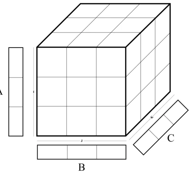
The board used for this thesis, does not contain enough BRAM resources to make computation on the real tensors. This is due to the storage requirement for factor matrices, namely, A, B and C matrices on BRAM. Performance-wise, it is too expensive to store the value on DRAM since the access pattern is random for the matrices. Therefore a solution is needed to make computation on the large tensors. The solution is to split the tensor into cuboids and process them separately so that the A, B and C matrices of the cuboids can be stored on BRAM for efficient random access.

5.2

Cache Blocking in Software

Cache blocking is used to increase the cache hit rate to improve performance significantly [47]. In cache blocking the operations are done in a chunk or block of the input to work on smaller memory space, in turn, this will dramatically increase the cache hit rates.

CHAPTER 5. TILING 20

5.3

Tiling for

MTTKRP Kernel

BRAM can be considered as a cache in FPGA since it is much faster than DRAM. A random access to the BRAM block can be done in one cycle whereas the memory access to DRAM can take several cycles. To achieve fast computation, i.e, process approximately one nonzero per one FPGA clock cycle, BRAM blocks must be utilized.

However, for most of the real tensor data, the A, B and C matrix sizes which depend directly on the dimensions of the tensor are so large that they won’t fit into the BRAM memory. Therefore either DRAM must be utilized with a huge performance loss or another technique is required.

Tiling can be used to split the tensor into cuboids so that the dimensions of the cuboids are small enough for A, B and C matrices can be stored in BRAM efficiently. Tiling is demonstrated in Figure 5.1.

5.3.1

Matrix Chunk sharing between iterations

In the cache blocked tensor MTTKRP kernel operates on the chunks of A, B and C matrices. If the tensors are in arbitrary order in each MTTKRP operation on a cuboid all factor matrices must be loaded and A must be written cumulatively from and to DRAM. However, this is also highly inefficient and the bottleneck becomes the memory accesses instead of the computation. Luckily the tensors are in order after the Tiling in the host so that consecutive tensors will share dimensions if they are not on the corners.

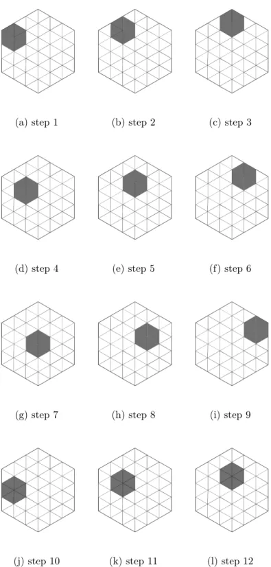
One simple way of exploiting this is to share A and B matrices and to alternate the C matrix across the subtensors. When the processed tensor is in the edge of the tensor, for the next iteration B value can also be read and when the tensor is in the corner, A value can be read for the next iteration together with B and C. This processing scheme is illustrated in Figure 5.2.

CHAPTER 5. TILING 21

5.3.2

Space Filling Curves

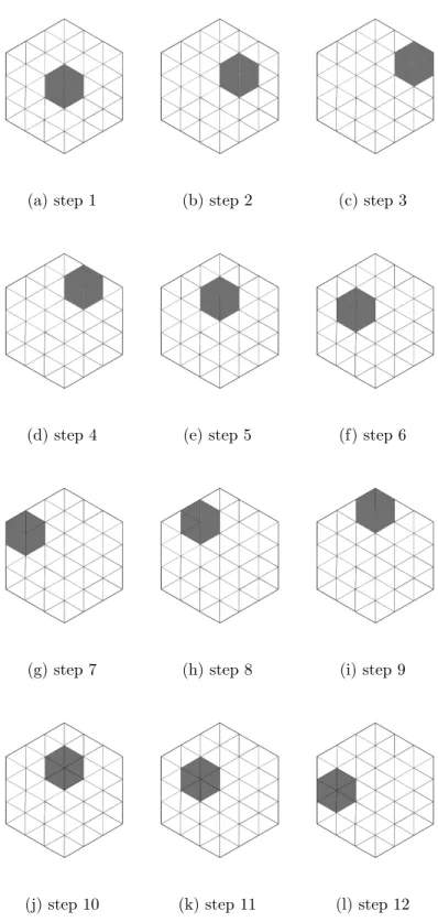
To minimize the DRAM communication and maximize the concurrent processing and accessing to DRAM, the order of processing the tensor is important. To maximize the performance a processing order scheme similar to the space-filling curves that have been utilized in [48] is used. In this scheme instead of processing the tensors in a triple for loop order, the processing order is implemented such that the next subtensor will always be the neighboring subtensor.

In this way, only one matrix chunk is needed to be brought to the BRAM while doing the computation. If the processing tensor is in the edge of the tensor, then B is read, if the processing tensor is in the corner of the tensor then A is read and in the next iteration, A is written to the DRAM. Otherwise, C is read. This order of processing is illustrated in Figure 5.3.

CHAPTER 5. TILING 22

CHAPTER 5. TILING 23

(a) step 1 (b) step 2 (c) step 3

(d) step 4 (e) step 5 (f) step 6

(g) step 7 (h) step 8 (i) step 9

(j) step 10 (k) step 11 (l) step 12

CHAPTER 5. TILING 24

(a) step 1 (b) step 2 (c) step 3

(d) step 4 (e) step 5 (f) step 6

(g) step 7 (h) step 8 (i) step 9

(j) step 10 (k) step 11 (l) step 12

Chapter 6

Methodology

6.1

Assumptions and Constraints

The kernel is implemented for integer value type. Therefore the tensors containing decimal values can only be approximated. Also, the tensors are required to be three dimensional. Higher-order tensors are not supported. The sub tensors which are the result of the tiling operation must be at most the size of 32768 × 32768 × 32768 and there can only be 2048 sub tensors due to the limitations on BRAM space on the board. Therefore very large dimensional tensors are not supported. There is no limitation on the number of nonzeros or sparsity.

6.2

Optimization Techniques

We have used the full bandwidth using memory banks. We have used loop pipelin-ing in every module and optimized the hardware so that the initiation interval (II) is 1 for the main computation loop. The writeOutput module was the most problematic since it requires a cumulative write operation on BRAM. Without

CHAPTER 6. METHODOLOGY 26

optimization, the II was 32 for this module. We have implemented pipeline for-warding so that the II can be reduced to 2. This means that in the computation part of the kernel, theoretically one nonzero can be processed in every 2 cycles if there is no contention on DRAM memory for the nonzero values that we are streaming from. Some other modules had problems with the II and they are also optimized by separating the memory access from the computation of the output values by utilizing either a BRAM buffer or an hls::stream.

6.3

The Kernel Structure

In software implementation, there is a triple loop. Outer loop goes through the slice indices, the second loop goes through the fiber indices and the inner one goes through the nonzero values. In HLS, since C code is written, it seems it is easy to ship the existing algorithm design to the FPGA, however, the performance of the kernel might be 100 times slower than the sequential baseline. Therefore instead of writing the code directly in HLS, a new design is proposed. This design exploits the distinct characteristics of the different arrays in the CSR-like storage scheme. Thanks to dataflow parallelism and hls::streams, it was possible to redesign the algorithm such that there is a single loop in the main computation. This design is explained in detail in chapter 6.3.1.

6.3.1

Kernel Modules

Tensor Computation

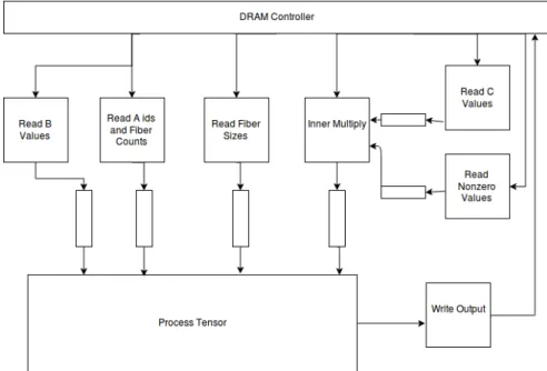
The tensor computation module is the core computation module of the kernel. In this module, the separate characteristics of the CSR-like format’s arrays are exploited. Each array is read separately by a simple extractor function that only reads the array and extracts the required value from the array and then sends it to the process_tensor module by an hls::stream. This way the design is simplified,

CHAPTER 6. METHODOLOGY 27

process_tensor has the data it needs to process the tensor and performance is maximized. The block diagram of the tensor computation module can be seen in Figure 6.1.

Process Tensor Process tensor is the main computation module of the ker-nel. It gets the required values from the hls::streams and then goes through the nonzeros instead of CSF data structures. In each iteration of the main loop, a nonzero is processed. It is assumed that there won’t be any empty fibers and there won’t be any fiber in the slice if the slice is empty. After the computation for a slice is finished in the process tensor, the computed value is passed to the write_output function via an hls::stream.

Read B Values Read B values module is responsible for fetching the B matrix’s rows in the correct order. It goes through the Fiber Indexes array’s js sub-parallel array and reads the corresponding B value of the j value that has been read from the DRAM.

Read C Values Read C values module is responsible for fetching the C matrix’s rows in the correct order. It goes through the Fiber Entries array’s ks sub-parallel array and reads the corresponding C value of the k value that has been read from the DRAM.

Read Fiber Sizes Read Fiber Sizes module is responsible for reading the fiber sizes of the existing fibers. It goes through the Fiber Indices array’s ptrs sub-parallel array and calculates the size of the fiber using the next value from the ptrs array then sends it to the process_tensor.

Read A ids and Fiber Cnts This module is responsible for both reading the slice index of the existing slices and reporting the count of fibers in that slice. To achieve this purpose it goes through the slice_indices array and determines if the

CHAPTER 6. METHODOLOGY 28

slice exists by examining consecutive values. If the values are different, then it means that the slice exists and the number of fibers can be calculated by getting the difference between the values.

Read Nonzero Values This module is only responsible for reading all of the nonzeros from Fiber Entries array’s vals sub-parallel array and push it into a hls::stream.

Inner Multiply The inner multiply module has a misleading name. It is the module that is in the innermost part of the algorithm and does a multiplication task. It gets the C value and corresponding nonzero value from the hls::streams and performs a multiplication operation. Then it sends the result to another hls::stream to be consumed by process_tensor.

CHAPTER 6. METHODOLOGY 29

RCW Pipeline

RCW (read-compute-write) pipeline module is the top-level module of the kernel. This module uses ping pong buffers to achieve concurrent compute and read-compute-write operations. When a tensor’s tile is being processed, the next tile’s data is concurrently getting fetched by the read module of the RCW pipeline. When a slice has been fully computed, the write operation is also concurrent with the computation operations.

6.4

Baselines

To understand the performance of the kernel, a variation of the the popular open-source tensor factorization tool Splatt [19] which is implemented by us.

6.5

Host Side Operations

To run the application on the FPGA some pre-processing steps need to be per-formed on the host computer. In the host, first, the input data is read from the file and loaded to the memory. After some statistical information such as dimen-sion counts and the nonzero counts are extracted to be used as parameters to the kernel. Then since the MTTKRP will be run only for one mode in the kernel and empty slices doesn’t matter the empty slices are removed. Tensors are normally stored with indices starting from one, however, this adds extra complication to the kernel, therefore it is decided to convert tensor indices to start from zero by subtracting one from each index in all of the nonzeros. This step is also done in the host.

After the first pre-processing steps, tiling is performed. After performing tiling operation the subtensors are converted into the Splatt format separately. All of the data including the meta-data of the tensors must be aligned to the 512-bit

CHAPTER 6. METHODOLOGY 30

memory scheme for the FPGA for efficient burst access from DRAM. Aligning is also performed in the host. Perhaps this was one of the most challenging parts of the implementation.

After the data is ready, SDAccel run-time is used to send data to the FPGA’s DRAM and execute the kernel. After kernel execution is done, the sequential baseline is run on the host as well. To run the baseline the Splatt format conver-sion must be done for the whole tensor too.

When the data is ready from both the kernel and the sequential baseline, the data is validated using sequential baseline results as the golden result.

6.6

Pitfalls of the design

There are some known pitfalls of the design. One of them is the distribution of nonzeros. For most of the real tensors, the data is not distributed evenly through the dimensions of the tensor. This will result in some very dense and some very sparse subtensors in the tiling operation. This will result in uneven computation times across the tiles and it will result in performance loss.

Another pitfall is processing of the empty subtensors. When the next subtensor has no nonzeros, the factor matrix rows for that subtensor is still being fetched with the current design. Since there is computation being performed concurrently it might seem harmless, however, when it is the empty subtensor’s turn, the system still needs to wait for the next subtensor’s data. This data can be fetched during the previous subtensor’s computation.

6.7

Future Improvements

The known pitfalls of the design can be addressed as follows. First, the uneven distribution of the data can be overcome by intelligent tiling such as utilizing

CHAPTER 6. METHODOLOGY 31

hypergraph partitioning, similar to Acer et. al’s work [15].

The empty subtensor problem can be overcome by more intelligent data loading during the computation.

The current design’s resource bottleneck is the BRAMs of the FPGA, however, the kernel still uses about 30% of the BRAM resources of the board, which means the kernel can be replicated at least 3 times to process chunks of slice dimension subtensors concurrently. Also, the C and B matrix chunks can be shared between the copies of the kernels which will further reduce the DRAM access counts and improve the performance significantly.

The current design utilizes one DRAM requests per cycle. Since 16 integers are coming in one DRAM request the design can perform almost 1 nonzero/cycle. However the DRAM interface can handle 4 requests per cycle, therefore if it can be fully utilized the kernel can be up to 4 times faster.

Chapter 7

Results

7.1

Input Data Description

Six tensors are used for the experiments. The information about the tensors can be found in Table 7.1

Tensor Name Number of Nonzeros dim1 dim2 dim3 Facebook-rm 738,078 42,390 1,506 39,986 brightkite 2,680,688 51,406 942 772,966 Enron-3 31,312,375 244,268 5,699 6,066 lastfm 186,479 1,892 12,523 9,749 movies-amazon 15,029,290 87,818 4,395 226,522 netflix 100,480,507 17,770 480,189 2,182 Table 7.1: Tensor information

7.2

Experimental Setup

Two computers are used in the experiments. The first one is called the many-core host. This computer is used to get the single-threaded baseline performance of our implementation of Splatt [19]. The other one is called the host. This PC is

CHAPTER 7. RESULTS 33

the host PC of the hardware accelerator board. The specs of the CPUs can be found in Table 7.2.

Host Many Core Host FPGA Host CPU Model E7-8860 [49] i5-7500 [50]

Number of Cores 18 4

Number of Threads 36 4

Frequency 2.20 GHz 3.40GHz Cache 45 MB 6 MB SmartCache

Table 7.2: CPU information

The FPGA tests are run in hardware acceleration kit Xilinx Virtex ultrascale vcu1525 board. The detailed information about the board can be found in Table 7.3

Model Virtex UltraScale+ FPGA VCU1525 [51] System Logic Cells (K) 2,586

DSP Slices 6,840

s Memory (Mb) 345.9

GTY 32.75Gb/s Transceivers 76

I/O 676

Table 7.3: FPGA information

The software baseline is a version of Splatt that is run on a single thread on the many-core machine with Xeon CPU. It was run for all of the tensors mentioned above with factor count 16 by varying the dimensions.

FPGA results are taken for factor count 16 for all of the tensors mentioned above by varying tiling factors and dimensions.

7.3

Kernel Performance

The most useful metric for measuring the kernel performance is to use the average number of cycles that have been spent for processing one nonzero in the kernel execution. This metric is calculated by using the throughput and the clock speed

CHAPTER 7. RESULTS 34

of the FPGA which is 300Mhz for all of the experiments and it is the main metric that we will be focusing on except for the actual runtime values where we compare it with the baseline runtime results.

In Figure 7.1, the average number of cycles needed to process one nonzero is shown per tensor across multiple experiments.

Figure 7.1: Average Cycle Per Nonzero On Tensors

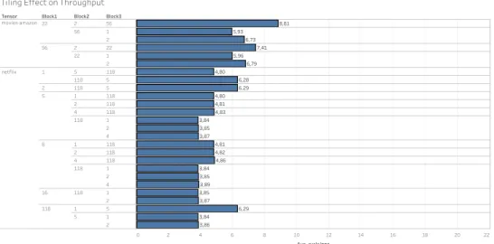
In Figure 7.2, the effect of tiling is shown in terms of the cycles per nonzero metric. As can be seen, the tiling has a negative impact on the performance since the number of DRAM accesses increases which becomes a bottleneck. Therefore the minimum tiling should be used for acceleration purposes.

The runtime comparisons with baseline are made for the minimum tiling which is allowed by the resources of the FPGA.

CHAPTER 7. RESULTS 35

Tensor Block1 Block2 Block3

0 2 4 6 8 10 12 14 16 18 20 22 Avg. cycle/nnz brightkite 1 189 13 13 189 13 1 189 189 1 189 1 13 13 1 enron-3 1 60 2 2 60 2 1 60 2 60 4 60 60 1 2 4 4 2 60 4 60 60 1 2 4 60 1 2 2 1 2 4 4 1 2 4 facebook-rm 1 10 11 11 10 2 10 11 11 10 4 10 11 11 10 10 1 11 2 11 4 11 11 1 2 4 11 1 10 2 10 4 10 10 1 2 4 lastfm 1 1 4 2 4 4 3 4 3 1 2 4 2 1 4 2 4 4 3 4 3 1 2 4 3 1 4 2 4 4 1 2 4 1 3 4 2 3 4 4 3 4 3 1 2 4 movies-amazon 1 56 22 22 56 2 56 22 22 56 2 56 14,57 14,59 15,65 19,98 16,99 20,03 5,60 7,40 7,39 7,41 7,45 6,16 6,49 6,49 7,44 7,55 6,20 6,70 6,50 7,10 6,20 6,24 6,50 6,35 6,11 6,52 5,04 5,14 6,87 7,05 9,92 10,27 5,45 7,52 10,92 12,59 9,40 7,50 5,48 7,53 10,94 12,52 9,41 7,46 7,22 7,36 7,19 7,00 7,16 6,77 6,90 7,22 7,54 7,36 7,18 7,40 6,80 6,82 7,32 7,79 6,90 6,51 6,47 6,78 7,06 7,08 8,08 7,97 8,18 6,41 6,25 7,01 8,52 7,26 8,70 Tiling Effect on Throughput

CHAPTER 7. RESULTS 36

Tensor Block1 Block2 Block3

0 2 4 6 8 10 12 14 16 18 20 22 Avg. cycle/nnz movies-amazon222 222 5656 56 1 2 56 2 22 22 1 2 netflix 1 5 118 118 5 2 118 5 5 1 118 2 118 4 118 118 1 2 4 8 1 118 2 118 4 118 118 1 2 4 16 118 1 2 118 1 5 5 1 2 8,81 6,73 5,93 7,41 6,79 5,96 4,80 6,28 6,29 4,80 4,81 4,83 3,87 3,85 3,84 4,81 4,82 4,86 3,89 3,85 3,84 3,87 3,85 6,29 3,86 3,84 Tiling Effect on Throughput

CHAPTER 7. RESULTS 37

7.4

Performance Comparison

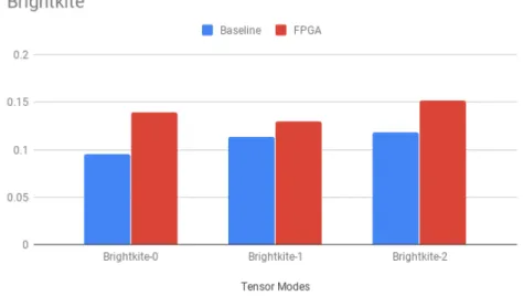
We have compared the kernel performance with the Splatt with a single thread on factor count 16. In the results, the labels are written as follows. The tensor name is written in the label followed by the slice mode. Slice mode is the mode where the horizontal slices are varying. This is the mode that corresponds to the output factor matrix. The modes are enumerated starting from 0 to 2 and the order of the modes is in the order of the dataset. The remaining two modes are selected by their length where the second mode is the shorter one and the third mode is the longer one. According to our experiments, this mode selection doesn’t matter for our FPGA implementation. In the Figure 7.3, the runtime comparison for Brightkite tensor is given. As can be seen the FPGA results are comparable with the baseline results, however, the FPGA is slower than the baseline for this tensor.

Figure 7.3: Brightkite Tensor Runtimes on Modes

In Figure 7.4, FPGA outperforms the baseline in all modes.

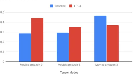
In figures 7.5, 7.6, 7.7 and 7.8 the runtime comparisons for Movies-Amazon, Lastfm, Enron3 and Facebook-rm tensors are given respectively. As it can be seen in the Figures the FPGA implementation is comparable with baseline and outperforms the baseline in at least one mode.

CHAPTER 7. RESULTS 38

Figure 7.4: Netflix Tensor Runtimes on Modes

Finally, in Figure 7.9, the speedup values are given for each tensor and mode combination.

CHAPTER 7. RESULTS 39

Figure 7.5: Movies-Amazon Tensor Runtimes on Modes

CHAPTER 7. RESULTS 40

Figure 7.7: Enron3 Tensor Runtimes on Modes

CHAPTER 7. RESULTS 41

Chapter 8

Conclusion

Tensor factorization is a very useful tool with many possible application areas. However, tensor factorization is a computationally expensive application. In this thesis, we have shown that the FPGA implementation of MTTKRP kernel is comparable with the current state of the art CPU implementations and it can be further improved to be even faster. Since MTTKRP kernel is the most time-consuming part of the PARAFAC algorithm and MTTKRP has many iterations on a single PARAFAC decomposition, FPGA accelerators can be used to improve the performance significantly.

Bibliography

[1] H. Lu, K. N. Plataniotis, and A. N. Venetsanopoulos, “A survey of multilin-ear subspace lmultilin-earning for tensor data,” Pattern Recognition, vol. 44, no. 7, pp. 1540–1551, 2011.

[2] H. Fanaee-T and J. Gama, “Tensor-based anomaly detection: An interdisci-plinary survey,” Knowledge-Based Systems, vol. 98, pp. 130–147, 2016. [3] M. A. PRADA, M. DOMÍNGUEZ, P. BARRIENTOS, and S. GARCÍA,

“Di-mensionality Reduction for Damage Detection in Engineering Structures,” International Journal of Modern Physics B, vol. 26, no. 25, p. 1246004, 2012. [4] A. Mnih and R. R. Salakhutdinov, “Probabilistic matrix factorization,” in

Advances in neural information processing systems, pp. 1257–1264, 2008. [5] S. Smith, J. Park, and G. Karypis, “Sparse tensor factorization on many-core

processors with high-bandwidth memory,” in 2017 IEEE International Par-allel and Distributed Processing Symposium (IPDPS), pp. 1058–1067, IEEE, 2017.

[6] S. Mittal, A survey of FPGA-based accelerators for convolutional neural net-works, vol. 1. Springer London, 2018.

[7] S. Yesil, M. M. Ozdal, T. Kim, A. Ayupov, S. Burns, and O. Ozturk, “Hard-ware accelerator design for data centers,” 2015 IEEE/ACM International Conference on Computer-Aided Design, ICCAD 2015, pp. 770–775, 2016. [8] D. Chen and D. Singh, “Fractal video compression in opencl: An

evalua-tion of cpus, gpus, and fpgas as acceleraevalua-tion platforms,” in 2013 18th Asia 43

BIBLIOGRAPHY 44

and South Pacific Design Automation Conference (ASP-DAC), pp. 297–304, IEEE, 2013.

[9] A. Cornu, S. Derrien, and D. Lavenier, “Hls tools for fpga: Faster devel-opment with better performance,” in International Symposium on Applied Reconfigurable Computing, pp. 67–78, Springer, 2011.

[10] “Vivado hls.” https://www.xilinx.com/products/design-tools/ vivado/integration/esl-design.html. Accessed: 2019-07-26.

[11] “Sdaccel.” https://www.xilinx.com/products/design-tools/ software-zone/sdaccel.html. Accessed: 2019-07-26.

[12] E. Acar, “CASTA2008,” no. September, 2015.

[13] A. Huy Phan and A. Cichocki, “PARAFAC algorithms for large-scale prob-lems,” Neurocomputing, vol. 74, no. 11, pp. 1970–1984, 2011.

[14] J. R. Gilbert, C. E. Leiserson, and C. Street, “P233-buluc.pdf,” pp. 233–244, 2009.

[15] S. Acer, T. Torun, and C. Aykanat, “Improving medium-grain partitioning for scalable sparse tensor decomposition,” IEEE Transactions on Parallel and Distributed Systems, vol. 29, no. 12, pp. 2814–2825, 2018.

[16] M. Potkonjak and W. Wolf, “Cost optimization in asic implementation of periodic hard-real time systems using behavioral synthesis techniques,” in Proceedings of IEEE International Conference on Computer Aided Design (ICCAD), pp. 446–451, IEEE, 1995.

[17] S. D. Brown, R. J. Francis, J. Rose, and Z. G. Vranesic, Field-programmable gate arrays, vol. 180. Springer Science & Business Media, 2012.

[18] Z. Bai, J. Demmel, J. Dongarra, A. Ruhe, and H. van der Vorst, Templates for the solution of algebraic eigenvalue problems: a practical guide. SIAM, 2000.

[19] S. Smith, N. Ravindran, N. D. Sidiropoulos, and G. Karypis, “SPLATT: Efficient and Parallel Sparse TensorMatrix Multiplication,” Proceedings

-BIBLIOGRAPHY 45

2015 IEEE 29th International Parallel and Distributed Processing Sympo-sium, IPDPS 2015, pp. 61–70, 2015.

[20] S. Smith and G. Karypis, “Tensor-matrix products with a compressed sparse tensor,” pp. 1–7, 2015.

[21] F. Z. Cheflali, A. Djeradi, and R. Djeradi, “Linear discriminant analysis for face recognition,” International Conference on Multimedia Computing and Systems -Proceedings, vol. 16, no. 1, pp. 1–10, 2009.

[22] J. Ye, “Generalized low rank approximations of matrices,” Machine Learning, vol. 61, no. 1-3, pp. 167–191, 2005.

[23] D. Xu, S. Lin, S. Yan, and X. Tang, “Rank-one projections with adaptive margins for face recognition,” IEEE Transactions on Systems, Man, and Cybernetics, Part B: Cybernetics, vol. 37, no. 5, pp. 1226–1236, 2007.

[24] J. Sun, D. Tao, S. Papadimitriou, P. S. Yu, and C. Faloutsos, “Incremental tensor analysis,” ACM Transactions on Knowledge Discovery from Data, vol. 2, no. 3, pp. 1–37, 2008.

[25] H. H. Mao, C. J. Wu, E. E. Papalexakis, C. Faloutsos, K. C. Lee, and T. C. Kao, “MalSpot: Multi2 malicious network behavior patterns analysis,” Lecture Notes in Computer Science (including subseries Lecture Notes in Artificial Intelligence and Lecture Notes in Bioinformatics), vol. 8443 LNAI, no. PART 1, pp. 1–14, 2014.

[26] K. Maruhashi, F. Guo, and C. Faloutsos, “MultiAspectForensics: Pattern mining on large-scale heterogeneous networks with tensor analysis,” Pro-ceedings - 2011 International Conference on Advances in Social Networks Analysis and Mining, ASONAM 2011, pp. 203–210, 2011.

[27] L. Shi, A. Gangopadhyay, and V. P. Janeja, “STenSr: Spatio-temporal ten-sor streams for anomaly detection and pattern discovery,” Knowledge and Information Systems, vol. 43, no. 2, pp. 333–353, 2015.

[28] A. C. Sobral, “Robust Low-rank and Sparse Decomposition for Moving Object Detection : From Matrices to Tensors UNIVERSITÉ DE LA

BIBLIOGRAPHY 46

ROCHELLE ÉCOLE DOCTORALE S2IM Laboratoire Informatique , Im-age et Interaction ( L3i ) Laboratoire Mathématiques , ImIm-age et Applications ( MIA ,” Book, no. May, 2017.

[29] A. Cichocki, D. Mandic, L. De Lathauwer, G. Zhou, Q. Zhao, C. Caiafa, and H. A. Phan, “Tensor decompositions for signal processing applications: From two-way to multiway component analysis,” IEEE Signal Processing Magazine, vol. 32, no. 2, pp. 145–163, 2015.

[30] F. Lotte, M. Congedo, A. Lécuyer, F. Lamarche, and B. Arnaldi, “A review of classification algorithms for EEG-based brain-computer interfaces,” Journal of Neural Engineering, vol. 4, no. 2, 2007.

[31] B. Blankertz, T. Ryota, S. Lemm, M. Kawanabe, and M. Klaus-Robert, “Optimizing Spatial Filters for Robust EEG Single-Trial Analysis,” IEEE SIGNAL PROCESSING MAGAZINE, 2008.

[32] L. He, C. T. Lu, H. Ding, S. Wang, L. Shen, P. S. Yu, and A. B. Ra-gin, “Multi-way multi-level Kernel modeling for neuroimaging classification,” Proceedings - 30th IEEE Conference on Computer Vision and Pattern Recog-nition, CVPR 2017, vol. 2017-Janua, pp. 6846–6854, 2017.

[33] D. Chen, Y. Hu, C. Cai, K. Zeng, and X. Li, “Brain big data processing with massively parallel computing technology: challenges and opportuni-ties,” Software - Practice and Experience, vol. 47, no. 3, pp. 405–420, 2017. [34] J. Dean and S. Ghemawat, “Mapreduce: simplified data processing on large

clusters,” Communications of the ACM, vol. 51, no. 1, pp. 107–113, 2008. [35] U. Kang, E. Papalexakis, A. Harpale, and C. Faloutsos, “Gigatensor: scaling

tensor analysis up by 100 times-algorithms and discoveries,” in Proceedings of the 18th ACM SIGKDD international conference on Knowledge discovery and data mining, pp. 316–324, ACM, 2012.

[36] N. Ravindran, N. D. Sidiropoulos, S. Smith, and G. Karypis, “Memory-efficient parallel computation of tensor and matrix products for big tensor decomposition,” in 2014 48th Asilomar Conference on Signals, Systems and Computers, pp. 581–585, IEEE, 2014.

BIBLIOGRAPHY 47

[37] J. H. Choi and S. Vishwanathan, “Dfacto: Distributed factorization of ten-sors,” in Advances in Neural Information Processing Systems, pp. 1296–1304, 2014.

[38] O. Kaya and B. Uçar, “Scalable sparse tensor decompositions in distributed memory systems,” in SC’15: Proceedings of the International Conference for High Performance Computing, Networking, Storage and Analysis, pp. 1–11, IEEE, 2015.

[39] S. Zhou, N. X. Vinh, J. Bailey, Y. Jia, and I. Davidson, “Accelerating Online CP Decompositions for Higher Order Tensors,” pp. 1375–1384, 2016.

[40] S. Smith and G. Karypis, “A medium-grained algorithm for sparse tensor fac-torization,” in 2016 IEEE International Parallel and Distributed Processing Symposium (IPDPS), pp. 902–911, IEEE, 2016.

[41] J. Antikainen, J. Havel, R. Josth, A. Herout, P. Zemcik, and M. Hauta-Kasari, “Nonnegative tensor factorization accelerated using gpgpu,” IEEE Transactions on Parallel and Distributed Systems, vol. 22, no. 7, pp. 1135– 1141, 2010.

[42] A. Abdelfattah, M. Baboulin, V. Dobrev, J. Dongarra, C. Earl, J. Falcou, A. Haidar, I. Karlin, T. Kolev, I. Masliah, et al., “High-performance tensor contractions for gpus,” Procedia Computer Science, vol. 80, pp. 108–118, 2016.

[43] Q. Yu, C. Wang, X. Ma, X. Li, and X. Zhou, “A deep learning predic-tion process accelerator based fpga,” in 2015 15th IEEE/ACM Internapredic-tional Symposium on Cluster, Cloud and Grid Computing, pp. 1159–1162, IEEE, 2015.

[44] N. D. Lane, S. Bhattacharya, P. Georgiev, C. Forlivesi, L. Jiao, L. Qendro, and F. Kawsar, “Deepx: A software accelerator for low-power deep learning inference on mobile devices,” in Proceedings of the 15th International Con-ference on Information Processing in Sensor Networks, p. 23, IEEE Press, 2016.

BIBLIOGRAPHY 48

[45] R. Andraka, “A survey of CORDIC algorithms for FPGA based computers,” pp. 191–200, 2004.

[46] “Loop pipelining and loop unrolling.” https://www.xilinx.com/ support/documentation/sw_manuals/xilinx2015_2/sdsoc_doc/

topics/calling-coding-guidelines/concept_pipelining_loop_ unrolling.html. Accessed: 2019-07-26.

[47] M. S. Lam, E. E. Rothberg, and M. E. Wolf, “{T}he {C}ache {P}erformance of {B}locked {A}lgorithms,” Proceedings of the Fourth International Con-ference on Architectural Support for Programming Languages and Operating Systems, Palo Alto, California, pp. 63–74, 1991.

[48] A. Heinecke and M. Brader, “Parallel matrix multiplication based on space-filling curves on shared memory multicore platforms,” pp. 385–392, 2008.

[49] “intel R xeon R processor e7-8860 v4 (45m cache,

2.20 ghz) product specifications_2019.” https://ark. intel.com/content/www/us/en/ark/products/93793/

intel-xeon-processor-e7-8860-v4-45m-cache-2-20-ghz.html. Ac-cessed: 2019-07-24.

[50] “intel R coreTM i5-7500 processor (6m cache, up to

3.80 ghz) product specifications_2019.” https://ark. intel.com/content/www/us/en/ark/products/97123/

intel-core-i5-7500-processor-6m-cache-up-to-3-80-ghz.html. Accessed: 2019-07-24.

[51] “xilinx virtex ultrascale+ fpga vcu1525 acceleration development kit_2019.” https://www.xilinx.com/products/boards-and-kits/vcu1525-a.html. Accessed: 2019-07-24.