Nonlinear energy transfer to short gravity waves in the presence of long waves

(1)

J . Fluid Mech. (1995), vol. 289, pp. 199-226

Copyright 0 1995 Cambridge University Press

199

Nonlinear energy transfer to

short gravity waves in

the presence of long waves

By

H.

S . OLMEZT A N D J. H. MILGRAM

Department of Ocean Engineering, Massachusetts Institute of Technology, Cambridge, MA 02139, USA

(Received 26 April 1994 and in revised form 29 November 1994)

Existing theories for calculating the energy transfer rates to gravity waves due to resonant nonlinear interactions among wave components whose lengths are long in comparison to wave elevations have been verified experimentally and are well accepted. There is uncertainty, however, about prediction of energy transfer rates within a set of waves having short to moderate lengths when these are present simultaneously with a long wave whose amplitude is not small in comparison to the short wavelengths. Here we implement both a direct numerical method that avoids small-amplitude approximations and a spectral method which includes perturbations of high order. These are applied to an interacting set of short- to intermediate-length waves with and without the presence of a large long wave. The same cases are also studied experimentally. Experimentally and numerical results are in reasonable agreement with the finding that the long wave does influence the energy transfer rates. The physical reason for this is identified and the implications for computations of energy transfer to short waves in a wave spectrum are discussed.

1. Introduction

In recent years, there has been increased interest in the energy balance of short sea waves because of the influence of these waves on microwave remote sensing of the sea surface. One component of the energy balance is the nonlinear energy transfer among differing wavenumbers.

It is well accepted that energy transfer in the energy-containing portion of a wave spectrum can be calculated by the method pioneered by Hasselmann (1962). This is a stochastic treatment of fundamental interactions between groups of four waves first studied theoretically by Phillips (1960). Both the fundamental theory and the stochastic application are based on a perturbation theory which presumes that wave amplitudes are small in comparison to wavelengths. This presumption is reasonably well satisfied by waves whose lengths and frequencies are close to those at the spectral peak. Most applications of the Hasselmann theory have been for waves whose frequencies are less than 2.5 times the spectral peak frequency. For typical spectral energy distributions, most of the energy transfer at a specified frequency comes from quartet interactions of waves in a relatively small frequency range surrounding the specified frequency (Hasselmann & Hasselmann 1985).

When short sea waves are considered, they generally exist in the presence of long waves whose amplitudes are not small in comparison to the short wavelengths. Two questions arise.

t

Present address : Bilkent University, Faculty of Business Administration, Bilkent 06533, Ankara, Turkey.

https://www.cambridge.org/core

. Bilkent University Library

, on

07 Feb 2019 at 07:54:17

, subject to the Cambridge Core terms of use, available at

https://www.cambridge.org/core/terms

(2)

200 H. S. Olmez and J. H. Milgram

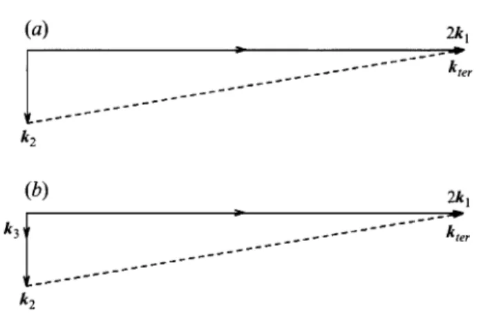
(a) 2k 1

k2

FIGURE 1. (a) Wave configuration for the special triad. (b) Wave configuration for the special

triad in the presence of an underlying long wave.

(i) To what extent is the nonlinear energy transfer to (or from) short waves due to interactions with waves with relatively similar frequencies altered by the presence of large waves with much lower frequencies and correspondingly longer lengths?

(ii) To what extent are the short-wave energy transfer results of computation methods based on small-amplitude expansions compromised by the presence of long waves?

In this paper we have answered these questions, in part, through computations and experiments on a set of interacting wave components both with and without the presence of an additional long large wave. The numerical studies comprise two approaches.

Our first approach is a direct numerical method which avoids perturbation expansions altogether. A time-stepping scheme is used to trace the evolution of water waves in a bounded domain. With prescribed initial conditions, the fully nonlinear boundary conditions are time-marched to determine the free-surface elevation and velocity potential in time. This requires knowledge of the normal velocity on the free- surface whose computation is numerically intensive and requires considerable computational resources. Our direct approach to obtain the normal velocity is to apply Green’s theorem using the Rankine source Green function and to solve the resulting integral equation at each time step.

The second numerical approach is a spectral method which utilizes small-amplitude expansions, but which includes perturbations of arbitrarily high order. It is along the lines of the spectral methods initially developed and used for other problems by Dommermuth & Yue (1987) and West et al. (1987). By comparing results from the two approaches, the accuracy of using the expansions is assessed.

Experimental confirmation exists for the theory of the growth of a short wave due to nonlinear interactions amongst intermediate-length waves in the absence of a large long wave (Longuet-Higgins & Smith 1966; McGoldrick et al. 1966). These experiments clearly showed the energy transfer and confirmed the initial growth rates given by the classical perturbation theory. Later Tomita (1989) repeated the experiments in a much larger wave tank to quantify the long-term evolution of the interaction. None of these experiments, however, addressed the accuracy of the perturbation scheme in the presence of a long large underlying wave. We conducted a laboratory experiment in which both a long wave and resonantly interacting intermediate-length waves were generated and we measured the growing short wave.

, on

07 Feb 2019 at 07:54:17

(3)

Nonlinear energy transfer to short gravity waves 20 1 Our experiment provides a basis of comparison for our numerical findings on the influence of the long wave on the nonlinear interactions amongst the intermediate- length waves.

A principal finding here is that a long wave significantly alters energy transfer to a short wave from intermediate-length waves with prescribed linear amplitude components. In addition to the numerical and experimental data, we are able to provide a physical explanation for why this occurs.

The results have implication for computations of nonlinear-energy transfer in a wave spectrum. This is complicated by the fact that the high-frequency tail of a measured wave spectrum is influenced not only by the usual linear wave spectrum proportional to the squares of wave amplitudes, but also significantly by the quadratic spectrum which depends on the fourth power of wave amplitude. In an appendix we derive expressions for the quadratic spectrum for unidirectional seas. Computations of nonlinear energy transfer in a wave spectrum require the full directional spectrum, but the simpler unidirectional spectrum is sufficient for showing that use of measured spectral values for computing nonlinear energy transfer to short waves must be done with care and caution.

2. The nonlinear wave-wave interactions

It is now well known that wave components exchange energy through nonlinear interactions. For gravity waves, the resonant nonlinear interaction generally requires a quartet of waves. The resonance conditions for the frequencies and wavenumbers under which these interactions take place can be written as (see Phillips 1960)

W 1 T W , T W , f W 4 = 0,

k , f k , f k , f k 4 = 0,

provided that the linear dispersion relation holds for each wave component:

W ; = g k n for n = 1 , 2 , 3 , 4 , (2) where g is the acceleration due to gravity. When the resonance conditions are satisfied, the third-order nonlinear interactions between three waves, which we call primary waves or primaries, result in a forcing function that has exactly the same frequency and wavenumber as the fourth. Since the fourth wave is a free wave, by virtue of its frequency and wavenumber satisfying the dispersion relation, it grows when forced at its own frequency and wavenumber, thereby obtaining energy from the other waves. The growing wave is called the tertiary wave. When the first three interacting waves, but not the fourth, are initially present, the amplitude of the tertiary wave, ater(t), behaves initially as

where K is the interaction (coupling) coefficient involving the wavenumbers, wave

frequencies and the first-order amplitudes of the first three wave components. Of all possible wavenumber configurations of the vectors k,, k,, k,, and k,, one is particularly convenient for theoretical and numerical studies. As illustrated in figure 1 (a), two of the primary wave trains coincide (say k,) and are perpendicular to another

(k,) so that there are only three distinct wavenumbers in the interacting resonant

quartet and the wavenumber of the resonant tertiary wave is given by

later(t)l = Kt, (3)

k,,, = 2k, - k,. ₍₄₎

, on

07 Feb 2019 at 07:54:17

(4)

202 H. S. Olmez and J. H. Milgram

The resonance conditions for this special triad require that the following equation along with (4) be also satisfied:

where the linear dispersion relation holds for each component. Combining the resonance conditions with the linear dispersion relation determines the theoretical ratio for the primary wave frequencies wJw2 = 1.73567 (Longuet-Higgins & Smith 1966). From the ratio of the primary wavenumbers, the tertiary wave is found to make an angle of 9.42" with k,. A prescribed wave frequency for one of the primaries defines the characteristics of the other members of the triad.

Phillips (1960) and later Longuet-Higgins (1962) studied this special triad utilizing perturbation theory and they derived theoretical predictions having the form of (3) for the initial growth of the resonant tertiary wave. This special case was also used as a bench-mark in the aforementioned experiments. In the theory of Longuet-Higgins

(1962), the fact that the tertiary wave grows at the expense of the primary waves is not

accounted for and the amplitudes of the primary wave components are treated as constants throughout the course of the interaction. For the set of waves in the canonical situation considered here, the initial growth rate does not continue since the tertiary wave interacts with the others once it has grown to finite size. Thus the physical interpretation of (3) should be restricted to a brief initial time which is small in

comparison with the interaction time. This limitation was overcome by Benney (1962) who showed that the energy sharing mechanism in the interacting quartet by analysing the full problem of energy exchanges amongst a set of four resonant waves satisfying (1). Based on the original work of Zakharov (1968) and the subsequent work of Crawford, Saffman & Yuen (1980), Stiassnie & Shemer (1984) derived a set of coupled nonlinear equations governing the evolution of the amplitude of each discrete mode involved in the quartet interaction up to third order. We shall see that to make the theory based on perturbations about the mean free surface accurate for the case at hand with the long wave, higher-order contributions from the spectral method are required.

In view of the wealth of background information on the interacting special triad, we used it as a 'base case' for our numerical and experimental investigations. Then we added the underlying long wave having wavenumber

k,

such that the wavenumber diagram took the form of figure l(b). Numerical and experimental studies were conducted on this set of waves. The important point here is that the long-wave amplitude is not necessarily small in comparison to the tertiary wavelength. By taking this approach we were able to assess the accuracy of the theoretical and numerical methods in addition to our principal objective which was determination of the influence of the long wave on the resonant interaction between the other waves. We found that the presence of the long wave modifies the growth of the tertiary wave, and why this happens.

wter = 2w,-w,, (5)

3. Numerical methods

A direct numerical method that avoids the perturbation theory approximation was developed by Olmez (1991) to compute the energy transfer for a quartet of waves. A spectral method program was also developed by us for further comparisons with the direct numerical method. The spectral method is a numerical application of perturbation theory, achieving numerical efficiency by using Fourier expansions in the horizontal domain, which includes perturbations of arbitrarily high order, thereby avoiding the third-order limitation of the conventionally used methods.

, on

07 Feb 2019 at 07:54:17

(5)

Nonlinear energy transfer to short gravity waves 203 For both methods, the approach taken is to consider flows governed by a velocity potential,

4,

satisfying Laplace's equation beneath a time varying free surface of elevation,

5.

The time evolution is determined by stepwise integrating the kinematic and dynamic free-surface boundary conditions :

3

= w(1 + O ~ . V ~ > - V ~ , . V C : on z =

c,

₍₆₎

at

where $s and w represent the velocity potential and the vertical velocity on the free surface. In the above equations, V = @/ax, a/ay) denotes the horizontal gradient. The time integration provides updated values of the surface elevation and velocity potential. In order to completely specify the flow so that a subsequent time-step integration can be carried out, the vertical velocity, w, must be found. The difference between the direct and the spectral methods lies in the way w is determined.

For our calculations with the spectral method, the time integration of the free- surface boundary conditions is carried out using a fourth-order explicit Runge-Kutta method with a constant time step. For the direct method, a fourth-order multistep Adams-Bashforth-Moulton method is preferred over Runge-Kutta owing to its computational efficiency since the numerical technique is computationally expensive. Various time-step sizes were tested in each of our calculations. A general finding was that a good time-step size is 2 to 3 % of the shortest fundamental wave period in the problem under consideration. No significant gains in accuracy were achieved with shorter time steps.

During the time-stepping procedure, a high-wavenumber instability on the free surface develops which, if not suppressed, eventually causes the numerical scheme to break down. This type of instability, often referred to as sawtooth, has been reported by several investigators (Longuet-Higgins & Cokelet 1976 ; Baker, Meiron & Orszag 1982; Dommermuth et al. 1988). We adopted a fast Fourier transform (FFT) technique by which all the high-wavenumber instabilities are filtered out. The surface wave elevation and the velocity potential are transformed into the Fourier space by a two-dimensional FFT, and all the higher-order harmonics that are above the wavenumber at which the instability is detected are filtered out. Then transforming back into the physical space by an inverse FFT, the computations are carried out for subsequent time steps.

3.1. Direct numerical evaluation

In our direct numerical procedure, the normal derivative of the potential is determined by solving the Green's theorem integral equation :

where the first integral is in the sense of a Cauchy principal value and excludes integration over the field point p . The singularity is located at the source point q.

G ( p , q ) = l/lrl is the three-dimensional free-space Green function where r = Ip-41 is

the distance between the source and field points.

The solution is carried out over the surface, S, of a domain defined by the calculated free-surface shape at each time and vertical sidewalls that intersect in a rectangular prism. With the resulting knowledge of the normal derivative of the potential, the vertical component can be calculated since the surface normal vector and values of the

, on

07 Feb 2019 at 07:54:17

(6)

204 H . S. Olmez and J. H . Milgram

potential on the surface are known. By alternately time stepping (6) and (7) and solving the integral equation (8), the surface elevation and the velocity potential as functions of time are obtained. After each time step, the two-dimensional Fourier transform of the free-surface shape is calculated to separate and evaluate the amplitude of the tertiary wave.

Since deep-water waves are considered, the computational domain can be freed of the bottom face provided that the domain is deep enough for there to be negligible flow at its bottom. Spatially periodic solutions are considered so that the boundary conditions on the side faces become periodicity conditions. We solve the integral equation (8) numerically by discretizing the boundary S into N quadrilateral panels,

and by satisfying the equation at a prescribed collocation point on each panel. Collocation points are chosen at the centroid of each panel where the boundary conditions are invoked. The simplest form is to consider the singularity strengths to be constant on each panel and each panel to lie in a plane. Each integral in (8) now depends only on the form of the Rankine source Green function, G, and the geometry of the panels. Explicit expressions for these integrals, which we have used in our numerical implementation, are given by Newman (1986). This direct numerical evaluation is also referred to as the boundary integral equation method (BIEM). Specific details of our BIEM are given in Olmez (1991) and in Olmez & Milgram (1995).

3.2. Evaluation by the spectral method

Dommermuth & Yue (1987) and West et al. (1987) developed high-order spectral

methods for the study of nonlinear gravity waves. These references provide complete descriptions so we only summarize the method here.

The spectral method also uses (6) and (7) to march the surface potential and elevation forward in time. It differs from the direct numerical method in the way it evaluates the vertical derivative of the potential after each time step.

The spectral method presupposes that the velocity potential can be expanded as a regular perturbation expansion in the following form :

where x = (x, y ) and M denotes the order of expansion adopted in the procedure. Following Dommermuth & Yue (1987), each Qm is further expanded in a Taylor series about z = 0 and the surface potential is obtained in the following form:

Expanding (10) and collecting terms at each order, provides the following sequence of equations for the unknown Gm in terms of the surface potential

os(x,

t ) :

@ l k 0, t ) = @&,

0,

(1 1)

The velocity potential at each order m (assuming periodic boundary conditions), for a

wave field composed of N free wave modes, is expressed by the following sum: N

Q m ( x , z, t ) =

C

$m, n(t)elkJzeikm.x, m = 1,2,.

. . ,

M , ₍₁₃₎

n=l

, on

07 Feb 2019 at 07:54:17

(7)

Nonlinear energy transfer to short gravity waves 205 where the k, are the wavenumber harmonics of the horizontal domain, k =

(kz,

kJ,

and deep water is implied. For each time, the modal amplitudes, & n , are found by

substituting (13) into (11) and (12), and solving for the unknowns as a function of lower orders. The vertical velocity is then approximated by the following expression :

Fast Fourier transforms are employed for moving back and forth between the physical and Fourier domains. For the time-stepping procedure, all the horizontal gradients of the surface potential and the wave height are performed in the Fourier domain. Starting with prescribed initial conditions for $s(x, to) and [(x, to), the free- surface boundary conditions are integrated in time over equally spaced collocation points, and the new values of the surface potential and the free-surface shape are computed in the physical domain. Based on the above approach, we prepared a computer algorithm for solving the nonlinear wave problems presented herein. 4. Experimental apparatus and procedure

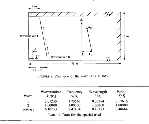
The experiments were carried out in a rectangular tank at the Institute for Marine Dynamics (IMD) of the National Research Council of Canada. The overall horizontal dimensions of the IMD tank are 75 m by 32 m and the maximum depth is 3.5 m. There are wavemakers on two adjacent sides of the tank with wave absorbers on the two remaining sides.

The wavemakers are segmented, with each segment hydraulically driven by a feedback control system so as to follow an applied electrical input signal. Each segment can have an arbitrary amount of piston-like or rotating flap-like motion. We operated the segments using piston-mode. All the segments on a single side were given identical motions to create intersecting (nearly) two-dimensional wave trains. Small amounts of leakage between adjacent segments result in small deviations from two-dimensionality

.

At the corner of the tank where the wavemakers would intersect, they are replaced by a solid rectangle which projects into the tank beyond the wavemakers by a = 0.185 m on one side and b = 0.675 m on the other side as shown in figure 2.

In order to test the linearity of the wavemaker system, waves from sinusoidal input signals in the frequency and amplitude ranges planned for the experiment were made by the wavemakers along one wall with those on the adjacent wall stationary. These waves were Fourier-analysed to assess their harmonic content. The ratios of the first and second harmonic amplitudes to that of the fundamental generally agreed with Stokes wave theory to within 1

YO

of the fundamental amplitude, although occasional errors up to 3% were observed. These errors correspond to 0.3 and 0.9 mm respectively. In all likelihood, they are due to variations in the shapes of the menisci of the water against the wave gauge wires which vary according to surface contamination. This was minimized by frequent cleaning.

Wave absorbers at the IMD facility are installed on the two tank sides opposite the wavemakers and are of the variable-porosity type described by Jamieson & Mansard (1987). Information from earlier tests done at IMD gives wave reflection coefficients of about 3% for the fundamental amplitudes and frequencies of our experiments. However, our data on the spatial variation of wave amplitudes indicate that the reflection coefficient could be as large as 10 %. The dominant resonant group involving reflected waves contains the original k, component and the reflected k, component. To

, on

07 Feb 2019 at 07:54:17

(8)

206

32 H . S. Olmez and J . H . Milgram

m 8 m

+-a-

Wavemaker I1

75 m *

FIGURE 2. Plan view of the wave tank at IMD.

Wavenumber Frequency Wavelength Period 1.735 67 0.33 1 94 0.576 15

1 3.012 55

2 1

.ooooo

1

.ooo

00 1.00000 1

.ooo

00

Tertiary 6.107 53 2.471 34 0.163 73 0.40464

TABLE 1. Data for the special triad

Wave lklllk2l W / @ z hlA2 T I T,

avoid an error from this effect, in our experiments the k, wave propagated in the long

tank direction and we used the data acquired before the reflected k, wave reached the wave gauges (see figure 2) in most cases (see below).

Measurements of the free-surface elevation were made by an array of resistance-type wave gauges made of two parallel 30-gauge copper wires spaced 1 cm apart. These wave gauges were calibrated by lowering and raising the wires through a known distance in calm water as well as by measuring sinusoidal waves with independently determined amplitudes. Five wave gauges were located at distances of 4.0,6.0,8.0, 10.0

and 19.7 m away from the wavemaker in the direction of the tertiary wave propagation over which the interaction takes place. According to the theory in $2, the tertiary wave at resonance is at an angle of 9.42" to the direction of the first primary wave (away from the second wavemaker with a slight component towards the first wavemaker). This generates a narrow reflection region from the first wavemaker. Hence the last wave gauge was located 9.07 m away from the first wavemaker to keep it out of the reflection zone. A plan view of the tank along with the gauge locations is shown in figure 2.

Measurements of the outputs from the five wave gauges were made with a 12-bit A- to-D converter and recorded on a computer in real time for subsequent data analysis. Each run consisted of 4096 points per gauge channel taken at a sampling frequency of 16 Hz which corresponds to 256 s of data, beginning 30 s after the wavemakers were turned on. At each sample time, all five channels were sampled in a time period of 0.04 ms (0.01 ms delay between channels). The 16 Hz sampling rate was chosen to avoid aliasing based on initial studies of measured data showing that spectral levels above 5 Hz were less than 0.5 % of the mean levels of the primary (k, and k,) waves. To maximize the dynamic range and the signal-to-noise ratio of the high-frequency

, on

07 Feb 2019 at 07:54:17

(9)

Nonlinear energy transfer to short gravity waves 207

tertiary wave data, the wave gauge system frequency response increased with frequency in the data range in a manner similar to that used by Olmez & Milgram (1992).

The wavemakers were operated with primary wave circular frequencies

w1 = 6.974 rad s-l and w2 = 4.018 rad s-' and as such the ratio w,/w, yields the theoretical value required for the resonant interaction. The long primary and swell (long wave) were generated simultaneously and propagated along the long side of the tank. The short primary wave propagated long the short side of the tank.

Spectral analysis was used to analyse the frequency distribution of wave energy at each wave gauge. The energy distribution in the wave field can be deduced from its power spectrum defined as

(15) where T is the length of the portion of the record used and z(t) is the data record from the measurements. The initial factor of 2 makes the spectrum one-sided. Tertiary wave amplitudes were computed at each gauge location from the integral of the surface elevation spectrum around the fundamental tertiary wave frequency :

a(@,,,) =

[2

S(w) dwll/l,

Wter-Aw

where Aw was chosen to be wter/50.

For a few runs, the entire 256 s record was divided into eight records, each 32 s long. These were individually analysed to determine the standard deviation of the measured tertiary wave amplitude. For the 32 s records, the standard deviation was 19.5 % of the tertiary amplitude.

Starting when the wavemakers are turned on, the tertiary wave reaches full theoretical growth at all wave gauges after 39 s and the reflection of the long primary wave from the tank wall absorber first reaches a wave gauge in 113 s. Therefore, the portion of the data shown in figures 4(a), 6(b) and 7 used in studying tertiary wave evolution was from 39 to 103 s after the wavemakers were turned on, corresponding to 9 to 73 s in the data records. This provided data sections of 1024 points for which the standard deviation of measured tertiary wave amplitudes is 13.8 %. For the cases shown in figures 4 ( b ) and 6(a), wave disturbances, probably related to wavemaker startup, evident in the early portions of the data record led us to analyse 1024 point data segments starting after the k, reflected wave reached the wave gauges.

5. Numerical and experimental results

We first consider the special triad alone and compute the growth of the resonant tertiary wave for primary wave steepnesses, e, of 0.1 and 0.2. The smaller steepness is used for benchmark purposes. Then, moderately steep waves are considered for testing the accuracy of the perturbation analyses. These numerical results are compared with our experimental measurements for the special triad. Then, a long wave whose amplitude is of the order of the tertiary wavelength is added to the special triad and the tertiary wave growth is computed under the influence of the long wave. These computations are also compared with the experimental results to confirm the validity of our numerical findings.

The tertiary wave amplitudes in the experiments are very small, typically a few millimetres. Although fractional differences between numerical results and experiment are sometimes substantial, in almost all instances the actual amplitude difference is less

, on

07 Feb 2019 at 07:54:17

(10)

208 H . S. Olmez and J . H . Milgram

than 1 mm. Of the 22 regularly analysed data points shown subsequently, 16 of them show differences in amplitude between experiment and computation of less than 1 mm. The remaining six points have differences between experiment and computation of less than 2 mm.

5.1. Results for the special triad alone

The special triad we will consider is composed of two primary waves

(k,

and k,) and the resonant tertiary wave as shown in figure 1. Based on the theoretical ratio of wave frequencies for resonance, table 1 summarizes the characteristics of each member of the triad.

The numerical solution to the boundary-value problem requires that the free-surface shape and the velocity potential be prescribed at the initial instant of time. We found that the numerical calculations are sensitive to initial conditions in that errors in them introduce standing waves in the system. We used perturbation theory to calculate initial conditions for the interacting triad up to second and third order in wave slope (Olmez 1991), with the latter naturally introducing fewer of the erroneous standing waves. Using these, the subsequent computations with the BIEM were fully nonlinear whereas the spectral method computations were carried out to the fifth order.

For the BIEM, the free-surface geometry is approximated by 32 elements in each direction. Along the depth, which is half the wavelength of the longer primary, 20 elements were used with a quarter-period cosine-spacing distribution, dense at the top. Filtering is applied at every time step such that wavenumbers above the eighth harmonic of the fundamentals are filtered out. With tenth-order filtering, a sawtooth appearance on the surface took over soon after one wave period of the long primary, at which point the departure from the initial energy and momentum was considerable. This does not occur with the eighth-order filtering.

For the spectral method, 64 elements are used in each direction on the free surface. This provides 32 unaliased modes in each direction. With this spatial resolution, convergent results are obtained with a fifth-order ( M = 5) approximation. Despite having fifth-order accuracy, Fourier modes up to the tenth harmonic of the fundamentals are preserved in the computations. Therefore, smoothing is applied at every time step such that wavenumbers higher than the tenth harmonic of the fundamentals are eliminated. A time step of TJ50 is used for both methods. Convergence with time-step size is examined in Olmez (1991) and At = TJ50 is found to be quite satisfactory.

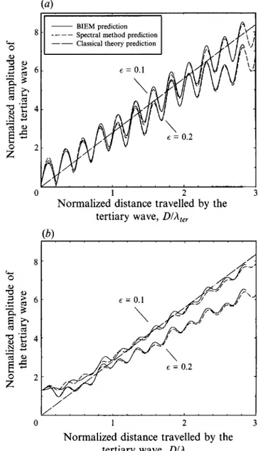
Figures 3(a) and 3(b) show our computed tertiary wave amplitudes for primary wave steepnesses of 0.1 and 0.2 with second- and with third-order initial conditions, respectively. The normalized amplitude, (ateJN, shown on the ordinates of the figures is

ater kter

( a t e r ) N = (a, kJ2(a2 k,) '

The theoretical results shown in the figures are based on ( 3 ) as given by the classical

theory (Longuet-Higgins 1962), and are normalized according to (17):

(ater)N = 2.77968 Dlhter, (18)

where D is the distance over which the interaction takes place.

Computations with our BIEM were performed only up to D = 3hter because of the computationally expensive nature of this numerical scheme. Note that the numerical computations display regular oscillations in the amplitude of the tertiary wave when the second-order initial conditions are used. These oscillations were much smaller when

, on

07 Feb 2019 at 07:54:17

(11)

Nonlinear energy transfer to short gravity waves (a> 8 rcl 0 w a w

.-

3 2 6 z3 g i 2 cd

.z

- g s 4

E

.Y c1

-

_p

2 0 1 2 3

Normalized distance travelled by the tertiary wave, Dlh,,,

(b)

209

0 1 2 3

FIGURE 3. Growth of the tertiary wave for (a) second-order initial conditions, and (b) third-order initial conditions.

initial conditions were accurate to the third order. An analysis of the relative phases between the first-order velocity potential and the wave elevation shows that these oscillations are consistent with their being due to standing waves. It is important to note that the oscillations are essentially identical for the entirely separate direct and spectral methods lending weight to the conclusion that they are associated with the initial conditions rather than numerical errors. For the nonlinear computations to be exact, purely travelling nonlinear waves are required for the initial conditions whereas we have used conditions for travelling waves up to third order.

For the second-order initial conditions, the tertiary wave starts with a zero amplitude whereas for the third-order initial conditions, the tertiary wave has a non- zero amplitude at t = 0. This is a steady-state, bound component which is in

, on

07 Feb 2019 at 07:54:17

(12)

210 H. S. Olmez and J. H. Milgram

quadrature with the growing component and whose existence is due to cross- interactions of the primary waves at the third-order as quantified by Olmez (1991). The growing tertiary wave component has a zero initial amplitude.

From figures 3(a) and 3(b), a comparison between the spectral method and the BIEM reveals that both methods are in remarkably good agreement. As a check on the global numerical accuracy of the BIEM, total energy and horizontal momenta are computed at every time step. These quantities are well conserved (to within 0.05

YO

and

0.1 % for the lower and higher steepnesses, respectively) during the entire simulation. For mild nonlinearities, the accuracy of the classical perturbation theory is good for the initial growth of the tertiary wave. For steeper primary waves, the accuracy of the perturbation approximation is restricted to a briefer initial time, which is consistent with the analysis of Tomita (1989).

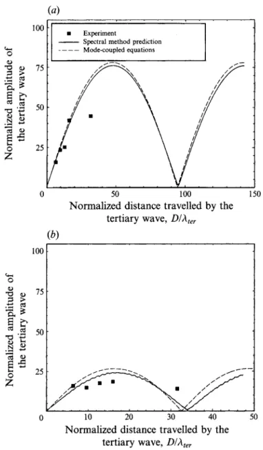
To provide a basis for the accuracy of the low-order mode-coupled equations in the long-term evolution of the wave field, we consider the results from the low-order mode- coupled equations (Stiassnie & Shemer 1984) and compare them with those from the high-order spectral method and from the experiment.

The modal amplitudes in the triad for the mode-coupled equations are obtained by solving a system of three nonlinear complex ordinary differential equations (Stiassnie & Shemer 1984, equation (4.1)) in time. A fourth-order Runge-Kutta method is employed with a time step of T,/120. The typical interaction distance needed for the tertiary wave to be comparable to a primary wave in size is predicted to be (Phillips

1960) :

Figures 4(a) and 4(b) show the long-term interaction of the special triad for two steepnesses. For both primary waves having a steepness of 0.1, the typical interaction distance requires 50ht,,. From figure 4(a), both the spectral method and the mode-

coupled equations predict the first maximum of the tertiary wave to occur near 48ht,, which closely corresponds to the theoretical interaction distance found above, Aside from a slight discrepancy in the maximum amplitude of the tertiary wave, mode- coupled equations performed well at this steepness. The higher-steepness case has

a, k, = 0.174 and a, k, = 0.180, which are the steepnesses achieved in the experiment.

For this case, the theoretical interaction distance reduces to 16h,,, because of stronger nonlinearity. The first maximum of the tertiary wave is predicted near 16.5ht,, and 1 7ht,, by the mode-coupled equations and the spectral method, respectively. Although

the mode-coupled equations do not completely agree with the spectral method for the entire simulation, the overall behaviours are similar. These comparisons validate the accuracy of mode-coupled equations for small steepnesses, with discrepancies being apparent at the higher steepnesses. Our experimentally observed amplitudes of the tertiary wave at the five wave gauge locations are also plotted in figures 4(a) and 4(b). Agreement between experiment and the numerical computation is quite good except for the last data point in each case which appears to be in error by about 1.9 mm in amplitude.

5.2. Results for the special triad on a long underlying wave

When a long wave whose amplitude is comparable to the tertiary wavelength is added to the wave field, the displacement from the equilibrium level for the tertiary wave will be on the order of its wavelength. This clearly violates the size restriction on the small expansion parameter of a perturbation expansion about the mean free surface for the short wave of interest. It would be possible to develop an expansion about the surface

, on

07 Feb 2019 at 07:54:17

(13)

100 43 0

4

a, 75-

.z

2

5 4 3

-25

'

.$

50- .5 + 21 1 -

FIGURE 4. A comparison of the mode-coupled equations with the spectral method and the experiment for primary wave steepness of (a) 0.1, (b) 0.174 and 0.180.

of the long wave to avoid this violation. On the other hand, we shall find that the same spectral method used above is accurate for the case at hand, in spite of the larger expansion distances.

The first objective here is to compute the initial tertiary wave growth under the influence of the long wave and make a comparison between results of the direct numerical method which has no size restriction and those methods that rely on perturbation analysis. Once we establish the validity of the more computationally efficient spectral method calculations, these will be used in predicting the long-term evolution of the tertiary wave for further comparisons with the experiments.

The long wave added to the special triad is chosen to be propagating in the same

, on

07 Feb 2019 at 07:54:17

(14)

212 H. S. Olmez and J. H . Milgram

Wavenumber Frequency Wavelength Period

Wave IklIlkA o l w z

v4

TI T,

3 0.25 0.50 4.00 2.00

TABLE 2. Characteristics of the long-wave component

direction as

k,

with a wavelength of 4 4 . Table 2 gives the characteristics of the long- wave component. The width of the computational domain in the y-direction is equal to the long wavelength along which we used 64 panels. This leaves 16 panels per wavelength for the longer primary wave which also travels in the same direction. The length of the domain in the x-direction is equal to the wavelength of the short primary wave, A,. The presence of the long wave makes this computational task quite a demanding one for the BIEM. Therefore, we used only 16 panels in the x-direction, maintaining the same spatial resolution for the primary waves. As before, 20 panels are used along the depth, which is now chosen to be half the wavelength of the long wave. Filtering is applied at every time step using fifth- and 17th-order filtering in the x- and y-directions, respectively. With our current spatial resolution, filtering at the above levels was needed to keep the simulation free of high-wavenumber instabilities. For the spectral method, we set the maximum order in the perturbation expansion to M = 5 and used 16 and 64 unaliased modes in the x- and y-directions, respectively, for the same computational domain. Filtering for the spectral method is also applied at every time step by removing the Fourier modes higher than the sixth- and 2lst-harmonics of the fundamentals in the x- and y-directions. As the BIEM is computationally expensive, we could not maintain the same spatial resolution in the BIEM as in the spectral method. This led to different filtering parameters in each approach. For both methods, At = TJ50 is used as the time-step size.

The initial conditions for this case are calculated by a third-order perturbation analysis. The presence of a fourth wave component makes the analysis ‘by hand’ onerously complicated. Therefore, the analysis for initial conditions was worked out to third-order using MACSYMA, a program that can handle algebraic manipulations

symbolically. Using MACSYMA, we also confirmed the results of our third-order ‘hand

calculations’ for the initial conditions of the special triad alone.

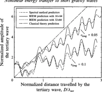
Figure 5 shows computed results and those from the classical theory which bases the growth rate on the initial amplitudes of the linear components. The steepnesses for the primary waves were chosen to be 0.1. The computations plotted in figure 5 were carried out for swell steepnesses of 0.05 and 0.1. The most important result is that the numerical methods show a large reduction in the growth of the tertiary wave when the long wave underlies the special triad. This is shown by both the BIEM and the spectral method. These two numerical methods show some local differences, but are in good global agreement.

Considering the relatively few control points used on the free surface for the run with the BIEM, it is essential to confirm the convergence with the spatial resolution. We could not double the number of control points on the surface as it was not computationally feasible. However, we were able to use twice as many panels in the x- direction and compute the tertiary wave amplitude for swell steepness of 0.1 as shown by the dotted lines. It follows closely the one with fewer panels. We found this convincing for the convergence, and did not perform the entire simulation.

In addition to the effects of small standing waves due to limiting initial conditions to third-order, figure 5 shows a periodicity in the growth rate with a period of 1.2 of

, on

07 Feb 2019 at 07:54:17

(15)

Nonlinear energy transfer to short gravity waves 213

0 1 2 3

FIGURE 5. A comparison of the spectral method with the BIEM in the presence

of an underlying long wave with steepnesses of 0.05 and 0.1.

the normalized units of the abscissa of the figure. This periodicity is also particularly

evident in the later figure 7. An analysis of the numerical system has shown that this is due to the time-varying phase differences of the long wave and the

k,

primary wave which propagate in the same direction. The computational domain length contains one long wavelength and four lengths of the k, wave. As time progresses, the long wave overtakes the

k,

wave by virtue of its larger phase velocity. This leads to a periodic time structure with period equal to A, divided by the difference in the phase velocities of the long and

k,

waves. This period is 1.56 s which corresponds to normalized distances of 1.23 units in the figures. The space-time transformation for these figures is based on the group velocity of the tertiary wave.

In view of the good agreement between the BIEM and the spectral method in the presence of the long underlying wave, we will use the spectral method to predict the long-term evolution of the tertiary wave for comparisons with experiment. Figure 6(a) and 6(b) show the tertiary wave amplitudes from the experiment and the spectral method. These figures also contain spectral method results for tertiary wave growth in the absence of the long wave to help demonstrate the effect of the long wave on tertiary wave growth.

In figure 6(a), the primary waves have a steepness of 0.1 and co-exist with a long underlying wave of steepness 0.05. The measured amplitudes at the three middle points are in good agreement with the results of the spectral method. The first point differs by an amount corresponding to 1.4 mm and the last point by 1.8 mm.

In the next run, whose results are in figure 6(b), we increased the steepness of the first and second primary waves to 0.174 and 0.180 respectively. The swell amplitude was kept the same. In this case, the numerical computation broke down after a time of 13.9 s which corresponds to a propagation distance of 11 tertiary wavelengths on the basis of the tertiary wave group velocity. At shorter distances, agreement between the measurements and the numerical results is reasonably good. In the more distant region, corresponding to times subsequent to breakdown of the numerical solution, the measured amplitudes are reduced.

The breakdown of the numerical solution might be the result of a physical instability

, on

07 Feb 2019 at 07:54:17

(16)

214 80 (c 0 w a w 1

2

6 0 - " a $ f i t ? .9 4 0 .

3 5

+

.-

+-I

H . S . Olmez and J. H . Milgram

0 Experiment (in the region computations failed)

-

(4

Spectral method prediction

80. _-

Spectral method prediction (no swell)

_.--.

__-.

,

,'

60 -

40-

associated with the combination of the swell and higher amplitudes of the primary waves. To test this possibility, we performed a two-dimensional BIEM calculation for the combination of the long primary wave and the underlying swell. We know (Olmez 1991) that our BIEM calculations can be taken very nearly to the point of physical instability and by taking a two-dimensional case, our computational resources allowed a long enough run. The BIEM computations broke down when used with the same spatial resolution and filtering parameters as in the three-dimensional case.

The interaction of the swell with the short primary wave induces a second-order bound component at a frequency of 20, - 20,. As the wavelength of the swell was four

times the wavelength of the long primary, the circular frequency of the swell turns out

, on

07 Feb 2019 at 07:54:17

(17)

Nonlinear energy transfer to short gravity waves 215

Experiment

Spectral method prediction

Spectral method prediction (no swell) - - 0

_ / - I.

.’

60 . ,’” /’ I f , / / / / 40 . /’ / 0 10 28 38

FIGURE 7. A comparison of the spectral method with experiment for primary waves of steepness 0.1 in the presence of an underlying long wave of steepness 0.075.

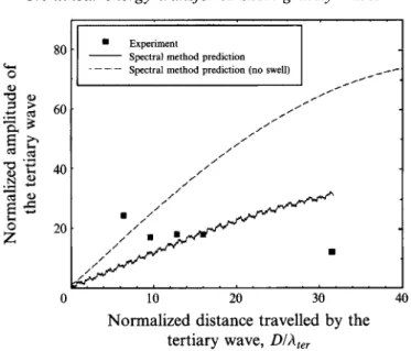
to be twice the frequency of the long primary. This makes the frequency of the second- order bound component the same as the frequency of the free-travelling tertiary wave. We calculated the magnitude of this bound component based on the third-order perturbation approximation. Although its contribution to the amplitude of the tertiary wave was found to be rather insignificant, we repeated the experiment with a different wavelength for swell that does not induce a bound component at the frequency of the tertiary. We selected a swell that has a wavelength of 5h, with a higher steepness of 0.075. This would have a more profound influence on the tertiary wave growth. We kept the primary wave steepnesses at 0.1.

Figure 7 shows the amplitude of the tertiary wave as measured at the five stations and compares it with the results of the spectral method. Spectral method results for the absence of the long wave are also shown for comparison. As expected, the reduction in the tertiary wave growth is more pronounced owing to the presence of a steeper swell. Again, the spectral method is in good qualitative agreement with the observed amplitudes for the three middle points. The first and last points have amplitudes that are different from the computations by 1.7 and 1.9 mm respectively. The experimental results are consistent with our numerical findings that the presence of a long underlying wave strongly influences the growth of the tertiary wave. In the last two sections, we consider the mechanism that leads to a reduction in the tertiary wave growth and discuss its implications.

6. Interactions leading to the reduction in tertiary wave growth in the presence of the long wave

In Olmez (1991), the perturbation expansion up to third order is given for the

interacting triad in the presence of the long wave. Although the purpose of this expansion was to set initial conditions for the subsequent computations, we can use it here to qualitatively interpret why the presence of the long wave reduces the growth of the tertiary wave. A close examination of the third-order interaction terms reveals that some of them have the same length and frequency as the first-order primary wave

, on

07 Feb 2019 at 07:54:17

(18)

216 H . S. Olmez and J , H . Milgram

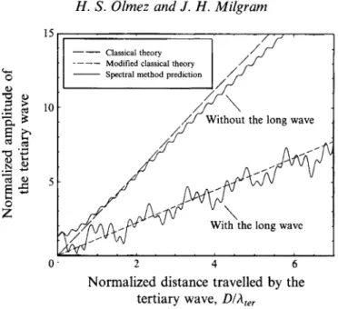
0 - 2 4 6

FIGURE 8. A comparison of the perturbation theory (based on altered amplitudes) with the spectral method in the absence and presence of the underlying long wave.

components. As a result, the sum of the elevations of the first- and third-order

components of the surface elevation of the nth primary wave (n = 1,2) has the form

+

AF,),(a,, k,)l cos (k, x - w,o, (20) where a, is the first-order amplitude and YM= 1 when n = 2 and vice versa. The

superscripts in parentheses denote the order. The A,,3 term is due to mutual interactions of the nth primary wave with the long wave, the A,,

,

term is due to mutual interactions of the nth primary wave with the mth primary, and the A,,

,

term is due to interactions of the nth primary with itself (Stokes effect). The correction to the first- order amplitude of a wave a&) due to its third-order interaction with another wave (21) a,@,) can be expressed as

A:;) = a, a; C(k,, k,,

O),

where 8 is the angle between the wave components. When the wave directions are within 90” of each other, the coupling coefficient, C, is always negative (Olmez 1991)

so it represents a reduction in wave amplitude.

The interaction is quite significant for the conditions of our experiments and numerical studies. For example, when all wave steepnesses are 0.1, the amplitude reduction of the first primary wave is 37 %. This results in a reduction in the tertiary wave growth by about 60

YO.

This relatively large effect occurs because a3 k, is not

small. When we examine the velocity potential of the first primary, we find a similar reduction in its component having the phase (k, x - w, t). The combined first- and third-order wave amplitude and the velocity potential components with this phase satisfy the linear free-surface boundary conditions to within 4

YO.

The implication is that the combined first- and third-order primary wave ‘looks like’ a smaller linear wave due to third-order interactions with the long wave. When we evaluate the theoretical growth rate from the classical theory (Longuet-Higgins 1962) using the reduced amplitudes of the primary waves in lieu of the first-order components, the result of this ‘prescription’ is in good agreement with the spectral method prediction as shown in figure 8.

L-2)

+

L-?

= [a,

+

AF,),(a,, 03, k,, k3)

+

A:,)&,, a,, k,, k,)

, on

07 Feb 2019 at 07:54:17

(19)

Nonlinear energy transfer to short gravity waves

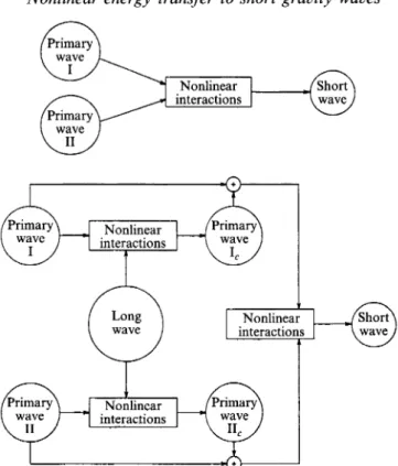
n

Primary 217 Nonlinear interactions W n No n I i n e a r interactions

FIGURE 9. Block diagram of nonlinear interactions of the special triad with and without the presence

of the long wave. Circles represent wave components. Boxes represent nonlinear interactions. The important interactions, both with and without the presence of the long wave are indicated diagramatically in figure 9. The upper part of the figure represents the interaction for the special triad alone. The primary waves interact nonlinearly to transfer energy to the tertiary wave. The lower part of the figure, which includes the presence of the long wave, is more complicated. Nonlinear interactions between the long wave and each primary wave generate a third-order wave having the same lengths and frequencies as the primary waves, but of opposite phase. They are indicated by I,

and 11, in figure 9. The elevation and velocity potential of each of these third-order components very nearly satisfy the linear free-surface boundary condition. Thus when these third-order components are added to their respectively first-order primary components, the results are very nearly the same as linear components of reduced amplitudes. The reduction is a significant fraction of the linear wave amplitude because the long-wave amplitude is so much greater than the amplitudes of the primaries. The same physical nonlinear interaction that exists for the special triad alone exists for the waves whose amplitudes have been reduced by third-order interactions with the long wave and this results in less nonlinear energy transfer to the tertiary wave than occurs in the absence of the long wave.

An alternative, although entirely complementary, explanation has been suggested to us by Professor Owen Phillips. The long wave modulates the amplitudes, frequencies and wavenumbers of the primary waves. Because of the frequency and wavenumber

modulations, parts of the primary waves go in and out of resonance with only the in- resonance part contributing to the energy transfer. The explanations are related because the modulated primary waves are composed of components with reduced amplitudes at the initial frequencies and wavenumbers and sidebands at the sum and

, on

07 Feb 2019 at 07:54:17

(20)

218 H . S. Olmez and J. H . Milgram

difference frequencies and wavenumbers. Only the components at the original frequencies and wavenumbers satisfy the resonance condition and contribute to the resonant interaction. This relationship is demonstrated in the growth rates shown in the examples. They contain a component with a period equivalent to 1.23 tertiary wavelengths which is the relative period between the long wave and the first primary. The growth rates go up and down as the system goes into and out of resonance at this period, with the mean rate of growth corresponding to the third-order-modified resonating components.

7. Implications for calculation of energy transfer to the high-frequency tail of a wave spectrum

The accepted method for calculating nonlinear energy transfer between frequency (or wavenumber) components of a gravity wave spectrum is based on the quartet interactions, but considered in a stochastic way. This is the method pioneered by Hasselmann (1962). The ‘input’ wave information is based on the linear components of the wave amplitudes. From the findings here, we would expect the calculated energy transfer to the high-frequency tail, based on resonant quartet interactions among linear wave components, to be an overestimate due to the presence of large long waves that are not part of the quartet. However, if the ‘input components’ are taken as the linear components plus the third-order amplitude modifications due to each component interacting with all the others, the estimate should be better. This issue has not been raised for most studies of nonlinear energy transfer because they deal mainly with the energy-containing portion of the spectrum, not the high-frequency tail. The latter is the part that exists ‘on top of’ much larger and longer waves.

When one measures ocean waves and separates the measurement into frequency or wavenumber components, each one corresponds to the complete component, not just the linear one. To calculate an estimate of the energy transfer distribution accurately in the high-frequency tail, it is desirable to know the linear and third-order components. This has led us to look into the relative sizes of the linear part of the wave

spectrum, Gll, which is O(A2) and the quadratic part of the spectrum, cBZ2

+

cBI3 which is O(A4). A is the linear wave amplitude. Gzz results from products of second-order wave amplitudes and G13 results from products of first- and third-order wave amplitudes. Our development is described in the Appendix.

Using the results derived in the Appendix, here we evaluate the quadratic corrections to a unidirectional sea spectrum whose linear components are taken from the spectrum model of Bjerkaas & Riedel (1979). This is not done for quantitative energy transfer calculations, which require a multi-directional wave field, but rather to demonstrate the importance of the higher-order contributions. One can argue, convincingly, that the high-frequency tail of the model spectrum contains all the higher-order corrections. However, using the model results as the linear spectrum suffices to show the importance of including the third-order amplitude effects when doing resonant energy transfer calculations, and of ‘weeding out’ the second-order influence which exists in measured spectra, when determining the first- and third-order amplitudes to be included. The important third-order component propagates at the same celerity as the linear component, but the second-order component at the same frequency has only half the celerity so it does not participate in the same resonant energy transfer interactions. We carried out the quadratic spectrum calculations for two wind conditions: (i) a 19.5 m wind speed of 5 m s-l with a friction velocity of u* = 0.163 m s-l, and (ii) a 19.5 m wind speed of 10 m s-l with a friction velocity of 0.362 m s-’. The friction

, on

07 Feb 2019 at 07:54:17

(21)

Nonlinear energy transfer to short gravity waves 219

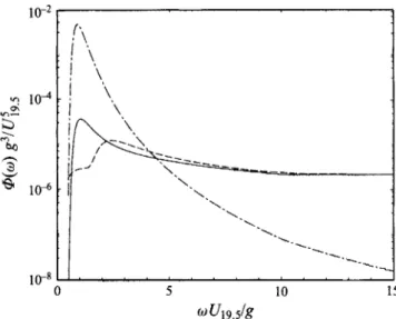
FIGURE 10. One-sided non-dimensionalized Bjerkaas-Riedel spectra : -

.-

, linear spectrum Gll;

--, quadratic spectrum 1GI31 (values are negative); ----, quadratic spectrum GZ2.

velocities were chosen by the methods given in Bjerkaas & Riedel(l979). Since U * / U ~ ~ . ~ differs for the two calculations, the resulting spectra need not obey a similarity law.

Nevertheless, when they are plotted in the non-dimensional form of figure 10 they are indistinguishable from each other. G13 dominates @22 in the frequency range of 0.5 to

2.0 times the spectral peak frequency. It is frequencies above this range that are of interest for our purposes here. There, the two quadratic spectral corrections are of

similar magnitude, with but of opposite sign. For

frequencies above about 4.5 times that of the spectral peak, the quadratic corrections to the spectrum exceed the ordinary linear spectrum so there the effects of still higher- order corrections might be important.

For resonant energy transfer interactions in which the energy-providing waves have frequencies less than 4.5 times that of the spectral peak, it is expected that the Hasselmann theory will be most accurate if wave amplitudes corresponding to Gll and

GI3 are used. The Q13 correction becomes important for frequencies higher than 2.5

times that of the spectral peak. When one measures the spectrum there appear to be two methods for separating out @22, which needs to be done to obtain the sum of Gll

and O13. One is to calculate all the components by methods similar to those given in the Appendix. This requires first extending the theory to the directional spectrum case. Alternatively, if the frequency-wavenumber spectrum is measured, @22 can be

determined through data analysis. The reason is that both Qll and Q13 will fall on the

first-order dispersion line, w2 = glkl, whereas @22 will not.

slightly greater than

8. Discussion and conclusions

The principal finding of this paper is that when a resonantly interacting quartet, or in particular the special triad studied here, exists on top of a large long underlying wave, the energy transfer in the resonantly interacting group is diminished from its value in the absence of the long wave. This was demonstrated, both numerically and experimentally, when the long wave propagated in the same direction as one of the ‘energy providing’ interacting waves called ‘primaries

’.

For the interacting special

, on

07 Feb 2019 at 07:54:17

(22)

220 H . S. Olmez and J. H . Milgram

triad, when a long wave of amplitude u3 and length about 25 times that of the growing tertiary wave, with u3 kter _z2.5, was present the tertiary wave growth rate was reduced theoretically to about 60% of its value in the absence of the long wave. The physical reason for this is that the nonlinear interaction between the long wave and the primary reduces the primary wave amplitude. Mathematically, this is a third-order interaction depending linearly on the primary wave amplitude and quadratically on the long-wave amplitude. Although our studies here were limited to a primary and a long wave propagating in the same direction, use of the interaction coefficients given in Olmez (1991) shows that when the two propagation directions are within 90" of each other, the primary wave amplitude is reduced.

The findings are of importance for calculating energy transfer to the high-frequency tail, and for that matter to the higher frequency portion of the 'equilibrium range' of measured or modelled wave spectra. The reason for this is that the measured spectra are influenced not only by the first-order wave amplitudes, but also by higher-order components, particularly for the high frequencies and wavenumbers. Our results suggest that the classical resonant energy transfer formulae should use the combined first- and third-order wave components as inputs to maximize high-frequency accuracy. Our study of the quadratic correction to the wave spectrum shows effects with similar orders of magnitude from first-third-order contributions and second-second-order contributions. These can be separated on the basis of theory or by data analysis if the frequency-wavenumber spectrum is known.

At wave frequencies higher than about 4.5 times that of the spectral peak, the magnitudes of the quadratic spectrum corrections exceed the magnitude of the spectrum resulting from linear wave components only. At these high frequencies, even higher-order corrections could be dominant.

A second finding is that numerical spectral methods for computing interactions between waves of different amplitude and wavenumber scales (q,

k,)

and (u2,

k2),

can be accurate even when u2kl is not small in comparison to 1. Results of the numerical spectral method are virtually identical to those of our fully nonlinear direct calculation in which the Green function integral equation is solved at every time step. The same reduction in tertiary-wave growth rate due to the long wave was found with our direct fully nonlinear method and by a spectral method which is based on perturbation theory, but which includes many interacting bound and free wave modes and which can accommodate an arbitrary order in the expansion (we used all orders up to and including the fifth). Evidently, the spectral method can be accurate for rather large values of u,k, if a sufficiently large number of modes and orders are retained.

Our experimental measurements are in reasonably good agreement with the numerical predictions. There is no systematic difference and the scatter in the experimental data suggests that differences between the numerical and experimental results are due mostly to experimental error.

This research was supported by The Office of Naval Research (Contract NOOO14-89-

J- 1 185) and The National Science Foundation (Grant OCE-9216788). Computations were made on a VAX 9000 at MIT; on a Cray-2 at the MIT Supercomputer Facility;

and on a Cray Y-MP at the Pittsburgh Supercomputing Center which is supported by The National Science Foundation (Grant OCE-900004P). The cooperation and assistance of the staff of the Institute for Marine Dynamics of the National Research Council of Canada is gratefully acknowledged.

, on

07 Feb 2019 at 07:54:17