MOTHBALLING IN THE ARMY
A THESIS
SUBMITTED TO THE FACULTY OF MANAGEMENT
AND THE GRADUATE SCHOOL OF BUSINESS ADMINISTRATION OF BILKENT UNIVERSITY
IN PARTIAL FULFILLMENT OF THE REQUIREMENTS FOR THE DEGREE OF
MASTER OF BUSINESS ADMINISTRATION
By
I certify that I have read this thesis and have found that it is fully adequate, in scope and in quality, as a thesis for the degree of Master of Business Administration.
--- Assist. Prof. Selçuk Caner
I certify that I have read this thesis and have found that it is fully adequate, in scope and in quality, as a thesis for the degree of Master of Business Administration.
--- Assist. Prof. Süheyla Özyıldırım
I certify that I have read this thesis and have found that it is fully adequate, in scope and in quality, as a thesis for the degree of Master of Business Administration.
--- Assoc. Prof. Hakan Berument
Approval of the Institute of Economics and Social Sciences
--- Prof. Kürşat AYDOĞAN Director
ABSTRACT
MOTHBALLING IN THE ARMY
BAYRAM BOZKURT
Master Of Business Administration in Management Supervisor: Assistant Professor Selçuk CANER
Modern armies mothball tanks, ships, planes, and vehicles. Up until now Turkish Army has not used mothballing. The surplus weapons are stored in arsenals. We just leave them idle vulnerable to rusting and try to keep them alive by maintenance; in fact we just let them die. The General Staff of the Turkish Army is planning to use mothballing, and giving an end to the wasting of unused weapons. This thesis proposes the use of real option modelling to be used in the mothballing decisions of military equipment for surplus in military hardware. Also, model can determine conditions for when to mothball, to switch back to full deployment status as well as abandonment of hardware.
ÖZET
TÜRK SİLAHLI KUVVETLERİNDE UZUN SÜRELİ DEPOLAMA
Bayram BOZKURT
M.B.A TEZİ
Tez Yöneticisi: Yrd. Doc. Dr. Selçuk CANER
Modern ordular tank, gemi, uçak, top gibi çeşitli silah ve teçhizatı uzun süreli olarak depolamaktadırlar. Şimdiye kadar Türk Silahlı Kuvvetleri uzun süreli depolama yapmamıştır. İhtiyaç fazlası silahlar depolara konulmakta ve sadece bakım yaparak faal halde tutulmaya çalışılmaktadır. Fakat bu yapılan bakım silahın kullanım ömrünün azalmasını engellememektedir. Uzun süreli depolama projesi sayesinde kullanım ömrü azalmadan silahlar depolanabilmekte ve ihtiyaç durumunda derhal kullanıma alınabilmektedir. Genel Kurmay Başkanlığı uzun süreli depolama projesini kullanarak
kullanılmayan silahlardan en üst düzeyde verim almayı hedeflemektedir. Bu tez kullanım fazlası silahların uzun süreli depolanmaları için bir model sunmaktadır. Ayrıca bu tezde silahların ne zaman depolanacağı, yeniden faaliyete geçirileceği, ve elden çıkarılacağına dair kıstaslarda verilmiştir.
ACKNOWLEDGEMENTS
I am very grateful to Assist. Prof. Selçuk CANER for his supervision, constructive comments, and patience throughout the study. I also wish to express my thanks to Assist. Prof. Suheyla ÖZYILDIRIM and Assoc. Prof. Hakan BERUMENT for showing keen interest to the subject and accepting to read and review the thesis.
TABLE OF CONTENTS
1. INTRODUCTION……….………..1
2. INVESTMENT DECISION………...…5
2.1.1. Payback Period………..6
2.1.2. Discounted Payback Period………...8
2.2.1. Internal Rate Of Return……….8
2.2.2. Modified Internal Rate Of Return………...……….10
2.3. Net Present Value………10
2.4. Real Options……….12
2.5. Mothballing………..………...13
2.6. Mothballing In The Army………....14
3. THE DECISION TO ENTER, EXIT, MOTHBALL, AND SCRAP……21
3.1. The Basic Model……….…23
3.2. Valuing The Project……….27
3.3. The Value Of The Project Under The Operating Cost And Temporary Suspension………..………..28
3.4. Thresholds In The Mothballing Option………..31
4. THE DECISION TO INVEST AND TO STAY IDLE………...35
4.1. Investment And Abandonment Thresholds………..35
4.2. Investment And Abandonment Thresholds For The Army………..36
4.2.1. The Effect Of Investment Cost On The Investment And Abandonment Thresholds………36
4.2.2. The Effect Of Abandonment Cost On The Investment And Abandonment Thresholds……….37
4.2.3. The Effect Of Risk-Free Rate On The Investment And Abandonment Thresholds………...……….39
4.2.4. The Effect Of Standard Deviation On The Investment And Abandonment Thresholds…...………..40
4.2.5. The Effect Of Operating Cost On The Investment And Abandonment Thresholds…………...……….41
5. THE DECISION TO MOTHBALL, TO REACTIVATE, AND TO SCRAP………..43
5.1. Mothballing, Reactivation, And Scrap Thresholds…..……….44
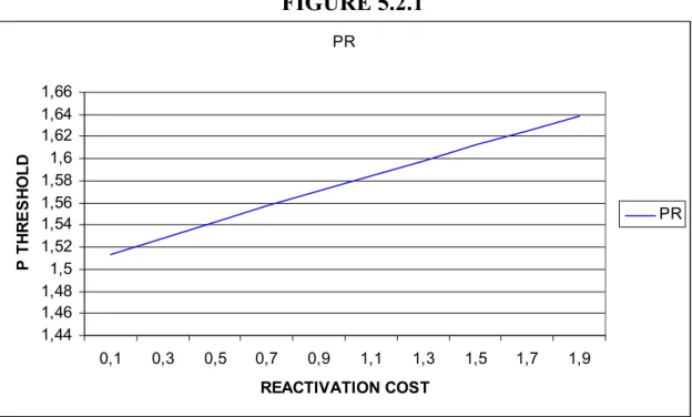
5.2.1. The Effect Of Reactivation Cost On The Reactivation
Threshold………...45 5.2.2. The Effect Of Mothballing Cost On The Mothballing
Threshold………...46 5.2.3. The Effect Of Maintenance Cost On The Reactivation And Mothballing Threshold……….………..47
5.2.4. The Effect Of Scrap Value On The Scrap Threshold……….49 5.2.5 The Effect Of Investment Costs On Thresholds…...……….50
5.2.6 The Effect Of Operation Cost On Thresholds………51 6. CONCLUSION………52 7. REFERENCES………54
LIST OF TABLES
2.1 Annual Costs Of Active Force And K-4 PMT………15 2.2 Maintenance Costs Of A Tank Division……….17 2.3 Depot Construction Cost For Mothballing A Tank Division………17 4.2 Costs For Mothballing A Tank Division………..36 4.2.1 The Effect Of Investment Cost On The Investment And
Abandonment Thresholds………..…………..…36 4.2.2 The Effect Of Abandonment Cost On The Investment And
Abandonment Thresholds….………..…………37 4.2.3 The Effect Of Risk-Free Rate On The Investment And
Abandonment Thresholds……….………...………38 4.2.4 The Effect Of Standard Deviation On The Investment And
Abandonment Thresholds………….………40 4.2.5 The Effect Of Operation Cost On The Investment And
Abandonment Thresholds………….………41 5.2 Costs For Mothballing A Tank Division………..45 5.2.1 The Effect Of Reactivation Cost On The Reactivation Threshold…45 5.2.2 The Effect Of Mothballing Cost On The Mothballing Threshold…46 5.2.3 The Effect Of Maintenance Cost On The Mothballing And
Reactivation Thresholds………48 5.2.4 The Effect Of Scrap Value Cost On The Scrap Threshold…………49 5.2.5 The Effect Of Investment Cost On The Thresholds………...50 5.2.6 The Effect Of Operation Cost On The Thresholds………51
LIST OF FIGURES
4.2.1 The Effect Of Investment Cost On The Investment And
Abandonment Thresholds……….………37 4.2.2 The Effect Of Abandonment Cost On The Investment And
Abandonment Thresholds………….………..…………..38 4.2.3 The Effect Of Risk-Free Rate On The Investment And
Abandonment Thresholds………...……….39 4.2.4 The Effect Of Standard Deviation On The Investment And
Abandonment Thresholds………41 4.2.5 The Effect Of Operation Cost On The Investment And
Abandonment Thresholds………42 5.2.1 The Effect Of Reactivation Cost On The Reactivation Threshold…..46 5.2.2 The Effect Of Mothballing Cost On The Mothballing Threshold…...47 5.2.3 The Effect Of Maintenance Cost On The Mothballing And
Reactivation Thresholds……….……49 5.2.4 The Effect Of Scrap Value Cost On The Scrap Threshold………….50 5.2.5 The Effect Of Investment Cost On The Thresholds………51 5.2.6 The Effect Of Operation Cost On The Thresholds………..52
NOMENCLATURE
α Drift parameter of simple Brownian Motion, or proportional growth rate
parameter of geometric Brownian Motion µ The risk-adjusted (CAPM) discount rate
δ Rate of return shortfall or convenience yield (µ – α) σ Standard deviation
r Risk-free rate
β Variable in fundamental quadratic. Its positive and negative roots are denoted
by β1and β2
A, B, D Constants of integration in solutions of differential equation C Operating cost of a project
I Capital cost of investment E Cost of Abandonment EM Cost of mothballing M Maintenance cost R Reactivation Cost ES Scrap Value PH Investment threshold PL Abandonment Threshold PR Reactivation Threshold PM Mothballing Threshold PS Scrap Threshold
1
1. INTRODUCTION
Modern armies mothball tanks, ships, planes, and vehicles. Up until now Turkish Army has not used mothballing. The surplus weapons are stored in arsenals. We just leave them idle vulnerable to rusting and try to keep them alive by maintenance; in fact we just let them die. The General Staff of the Turkish Army is planning to use mothballing, and giving an end to the wasting of unused weapons. This thesis proposes the use of real option modelling to be used in the mothballing decisions of military equipment for surplus in military hardware. Also, model can determine conditions for when to mothball, to switch back to full deployment status as well as abandonment of hardware.
Armed forces are characterized according to their readiness to war. The term “readiness” means “the ability of forces, units, weapon systems, and equipment to deliver the outputs for which they were designed”. Implicitly, readiness is to have the capability to engage in a military action including the deployment of forces in a reasonable amount of time that will protect national interests.
Due to its location, Turkey’s defense strategy was formed on mass army structure, which could meet the enemy in more than one front simultaneously. The major part of the defense manpower system is enlisted personnel. In the draft system, enlisted personnel are drafted from the male population at the age of twenty and over. In a draft system, one key goal is to preserve equity among the draftees. There is no difference in compensation between a highly skilled productive draftee and an ineffective one. The inadequate compensation often discourages skilled labor from undertaking additional responsibilities and generally, there is a tendency to avoid work. The goal of a draftee is to complete the duty as soon as possible with the least effort while the organization’s goal is to achieve a certain level of defense by using the draftees at hand. The gap between the goals of a draftee and the defense organization is so wide that often supervision is required to accomplish the defense mission. Since most of the draftees are reluctant to do the mission the efficiency and the readiness of the army are not at the level that is needed for defense. The dedication to task is low; the medical and the administrative expenditures are high.
2
There are discipline problems occurring among the reluctant draftees; the morale is low. Since the draftees are not seen talented, complex, high-tech weapons are not used and simple weapons are preferred.
Nowadays the existence of mass armies is highly debated. The answer is very complex because the revolutionary modernization of military technology and the expansion of the scope of requirements set for the soldiers have increasingly signaled that the military activity following the societal and technological development has been going professionalisation. The growing division of labor and increasing need for specialized qualifications and abilities have called for an effective force well trained and ready to serve for a long period. For market-oriented societies, it has become very important to achieve a higher return from investments in this sphere as well. From this point of view, mass armies have become more and more uneconomical. The entire situation has become even more complex by the fact that the nature of threats and the range of instruments to tackle them have changed in the last several decades. Experts have been recognizing that big-size armies can be interoperable only with great difficulties, and can no longer meet the task of managing new defense risks. But in defending the territory, the sovereignty and the values of the country still remains as an important objective.
The need for a professional, flexible, and effective army is apparent now. “Recently, the Army Chief of Staff presented a new vision for a much lighter and more rapidly deployable Army1”. Professionalism has its own costs. In peacetime, unnecessary mobilization of forces will exhaust national resources. Therefore, there must be a downsizing of the military. Defense capability should be measured in terms of not only active forces but also reserve, civilian, and allied forces.
In the case of a downsizing, we will face with the problem of surplus weapons, equipment, and vehicles. There are options to handle this problem:
• Mothballing of weapons is simple but it comes with a price. Mothballed weapons must be safeguarded, and may be deployed or sold in the future.
1 Uzun Süreli depolama Projesi,2001, Genel Kurmay Başkanlığı kara kuvvetleri Komutanlığı, Lojistik
3
• Export of surplus weapons is the economically most attractive solution, but potentially the most irresponsible. Currently, considerable quantities of surplus weapons are sold on the world market.
• Allowing the weapons to become obsolete over time is a consequence of insufficient storage technologies. It entails considerable environmental risks.
• The destruction of weapons is technically feasible, although there are severe ecological risks and high economic costs.
• Conversion of weapons or other military equipment for civilian use is mostly limited to specific military equipment categories (such as radar, trucks, helicopters, small boats, etc.).
• Partially 'demilitarized' weapons may serve for other military purposes-for example, as simulators, targets, or exhibits
Every year large sums from the budget are spent to maintain a peaceful environment. Frequently, public debate focuses on the expenditures of the Army. People living in the country cannot see the benefits of the investment in military hardware unless there is a war, and they think that the share of the Army from the budget should be reduced. The Turkish Army should be very careful in allocating resources for investment, and should abandon older investments, that are not beneficial.
Dixit and Pindyck (1994) studied the mothballing in the oil tanker industry. Oil tanker would be a good example for the Turkish Army because there are lots of similarities. The potential or actual owners of oil tankers face considerable profit uncertainty, as well as substantial sunk cost. The geographical distribution oil production and consumption fluctuates due to the environment. Nowadays we can observe the fluctuations in the oil prices; the probability of war increased the oil prices. The fluctuations in the oil prices increase the uncertainty making the oil tanker investors worry about the investment decisions.
4
Army, as an investor, shares similar anxiety; she makes investments but there are some uncertainties in the environment. The dilemma of the army is: The assets that she invested can only be used in case of a war and if she does not invest in them her defense could be in danger. At peace, she does not use her assets, but she cannot abandon them since she could need them in the future.
The Turkish Army has not used the mothballing option in evaluating her defense expenditure decisions until now. This study will give a new insight to the evaluations of the investment decisions. In this study, we examine the mothballing option of military equipment and try to find out whether it is a beneficial alternative for the Turkish Army or not.
5
2. INVESTMENT DECISION
“Economics defines investment as the act of incurring an immediate cost in the expectation of future rewards”.2 The object of the investment decision is to find real assets, which are worth more than they cost. The Turkish Army is an investor in this sense because she invests in arms, vehicles, and technology in defense of the Turkish Republic. The output of such investment is a secure country where people live in freedom.
“A firm that shuts down a loss-making plant is also “investing”: the payments it must make to extract itself from contractual commitments, including severance payments to labor, are the initial expenditure, and the prospective reward is the reduction in future losses”2. The Turkish Army abandoning the use of an old, ineffective weapon system is also investing because she cannot reach her goals by using ineffective hardware.
Irreversibility, uncertainty, and timing of the investment project effect the decisions of the investors. Investment expenditures are largely irreversible; once an investment is made it becomes more or less a sunk cost that cannot be recovered. The Army invested in a special type of gun and vehicle to build a defense system and have spent lots of money. She trained her personnel, and designed her defense system according to her investments and she cannot change them immediately. The investments are irreversible and the expenditures are sunk costs.
There is uncertainty over the future gains from the investment. The technology is changing continuously and everyday a new type of weapon or ammunition is developed which is superior to the prior one. Countries invest in their defense system according to their possible enemies. If the enemy has a superior missile system and if your anti-missile system cannot protect the country you have to invest in new anti-missile systems. You have to follow a dynamic investment procedure to keep in touch with the needs of your country.
2 Dixit A K and Pindyck R S, 1994, Investment Under Uncertainty (Princeton, NJ: Princeton University Press).
6
The timing of the investment is also very important. An investor can postpone investment if she thinks that there is no need for a superior system because there is not a hostile environment, which threatens the country. Investing in a new weapon system at a peaceful environment can trigger an arms race among neighboring countries.
There are some techniques which will help us decide whether invest or not, whether invest now or later and whether mothball or abandon. Computing the value of the investment under different possibilities can help us solve these issues. Measures commonly used to determine the value of an investment are:
• Payback period / Discounted payback period
• Internal rate of return / Modified internal rate of return • Net present value
• Real Options
2.1.1. PAYBACK PERIOD
The calculation of payback period is the simplest method for evaluating the investment decision. The payback method simply calculates how many periods into the future it takes for an investment project to repay the initial investment. The logic behind the payback rule is as follows. First, the faster the initial investment is returned, the shorter the time that firm’s capital is put at risk. There is less time for unexpected adverse events, which may result in a loss. Shorter payback can be said to proxy for lower risk. Second, a project that has a high early cash flow is more valuable because you can reinvest them. A payback period is usually expressed in months or years and represents the time that the inflows will recover the initial outflows. If the payback period is much less than the economic lifetime of the project, then the project is considered acceptable. The payback method is easy to compute and it favors the liquidity of the firm. It considers short-term investment horizon and limits the risk exposure of the firm. The payback method has also some
7
disadvantages. First, the payback method treats all cash flows prior to payback as equal; it ignores the time value of the money. We know that “a dollar today is more than a dollar tomorrow”3. Second, it ignores all cash flows subsequent to payback, no matter how large these might be. An investor will tend to accept poor short-lived projects and reject more profitable long-lived projects. Thus, although simple and easy to use, the payback method is generally deficient for evaluating investment projects.
We can evaluate the investment decision of a firm by using payback period. Let’s assume that a firm has two investment opportunities. Their cash flows are given below: YEARS 0 1 2 3 4 CASHFLOW A (100) 30 20 50 100 CASHFLOW B (100) 50 30 20 0 CASHFLOWS PROJECT A=100=30+20+50 PROJECT B=100=50+30+20
If the firm applies payback rule in her investment decisions A and B would be considered equal; both of them have a cutoff date of three years. But we can easily observe that project B generates more cash flow in the first year. Since the payback rule does not appreciate the time value of money a decision maker will ignore this crucial knowledge if she only depends on payback rule. We can also observe another crucial shortcoming of the payback rule in our example: since the cutoff date is three years a decision maker who has chosen project B according to the payback period will fail to see the cash flows after the cutoff date and make a mistake by considering the two projects equal.
3 Richard A. Brealey, Steward C. Myers, 2000, Principles of Corporate Finance, Sixth Edition, McGrow-Hill Higher Education.
8
2.1.2. DISCOUNTED PAYBACK PERIOD
The discounted payback method attempts to correct one of the shortcomings of the payback method, the time value of the money. The inflows are discounted to reflect the value of time. But it fails to take into account all of the inflows generated by the project. Once the discounted payback period is found, cash flows subsequent to that period are not taken into account. Let’s evaluate an investment decision by using discounted payback period.
YEARS 0 1 2 3 4
CASHFLOW A (100) 30 40 55 100 CASHFLOW B (100) 68 30 20 0
The discounted payback rule does not give equal weights to cash flows before the cutoff date. If we use a discount rate of 10% we will see that both projects have a cutoff date of three years.
DISCOUNTED CASHFLOW A 30/1.1 + 40/1.12 + 55/1.13 101.65 DISCOUNTED CASHFLOW B 68/1.1 + 30/1.12 + 20/1.13 101.65
But we can observe that discounted payback period failed to take into account the cash flow after the cutoff date just like the previous method. An investor who has chosen a project according to discounted payback rule would consider the two projects equal and would fail to see the cash flows after the cutoff date just like the fourth year cash flow of project A.
9
2.2.1. INTERNAL RATE OF RETURN
The internal rate of return is simply the discount rate that equates the net present value of the future cash flows from an investment project equal to zero. In other words, it is the yield to maturity. It is often difficult to determine the rate at which future cash flows should be discounted to today’s value. The internal rate of return (IRR) is a method for determining the value that does not depend on a discount rate and that expresses value in terms of a percentage. Decision makers are often more comfortable with value which is expressed in percentage terms. If you know the opportunity cost of capital you can make a comparison between the IRR of your investment and the return of the other opportunity. The decision to accept or reject a project depends upon whether or not the IRR exceeds the other rate. If the IRR is higher than the other one you should invest, if not you should choose the other opportunity. The IRR method is widely used but it has some conceptual problems. The IRR is difficult to interpret and it does not measure increases or decreases in wealth. When ranking projects IRR does not guarantee the maximization of firm’s wealth and projects with unusual cash inflows may have multiple IRRs. Difficulty arises when calculating the IRR of a project that has expenditures after the first period. Due to the mathematics of the calculations it is possible to calculate multiple IRRs that equate the net present value of inflows with the net present value of outflows. IRR rule also does not discount at opportunity costs of capital. It assumes that the investor can reinvest his money at the IRR, which is different from the market determined opportunity cost.
Let’s evaluate an investment decision by using IRR rule.
YEARS 0 1 2
CASFLOW A (1389) 800 800
IRR OF THE PROJECT 1389=800/ (1+IRR) +800/ (1+IRR) 2
10
If an investor was asked, “What is the return on this investment?” it is obvious that the answer is 10% because for every dollar invested, he gets $1.10 back. If the investor has alternative opportunities he would choose the one with the biggest IRR to make a better profit.
2.2.2. MODIFIED INTERNAL RATE OF RETURN
Modified internal rate of return (MIRR) is a technique that allows for the calculation of an internal rate of return when expenditures occur after the initial period. The method requires the compounding of all cash flows to the last period of the project at a given discount rate. Once the cash flows have been compounded forward MIRR, which equates the net present value of the future cash flows from an investment project to zero, can be calculated. Let’s evaluate an investment decision by using MIRR rule:
YEARS 0 1 2 3
CASFLOW A (663) 800 400 (400)
Let’s assume a discount rate of 10%:
MIRR OF THE PROJECT: 800*1.12 + 400*1.1 – 400 = 1008
663 = 1008/ (1+ MIRR) 3 MIRR= 15%
2.3 NET PRESENT VALUE
To evaluate investment projects correctly, we need a method that recognizes the time value of the money, and takes all cash flows into account. Traditionally, investment decisions have been evaluated using Net Present Value (NPV) approach, wherein discounted future net cash flows are added to the initial
11
investment to assess the likely impact of the project on shareholder wealth. The NPV of an investment is the sum of the present values of all inflows and expenditures expected to be associated with the investment. A positive NPV signals an opportunity that will add to wealth, and the NPV rule recommends that if the discounted inflows are more than the outflows undertaking the investment is beneficial.
There are some problems in using the NPV approach. The outflows can be computed easily but there will always be some uncertainties in computing the inflows. Nobody can know what will happen in the market for sure. The discount rate, which should be used in calculating the present value, is also a matter of problem. Solving issues like these are important topics, but the basic principle is fairly simple; calculate the NPV of an investment project and see whether it is positive.
Using the NPV rule implies that firms have static expectations. It expects that it is going to sell certain amount of products at certain prices and it is going to incur certain expenditures. It assumes that the inflows and outflows of the firm are certainly known and NPV can be computed using a discount rate.
Another assumption of the NPV approach is that investment is largely reversible and investment opportunities are once-and-for-all. Since this assumption implies that sunk costs can be recovered they do not matter for the investment decision. Since the investment is reversible, it can somehow be undone and the expenditures can be recovered if market conditions turn out to be worse than anticipated. If the investment is irreversible, it is a now or never proposition, that is, if the firm does not undertake the investment now, it would not be able to invest in the future. If the NPV of a project is negative they do not even think about investing after a while when conditions change. To demonstrate, let’s evaluate an investment decision by using the NPV rule:
YEARS 0 1 2 3
CASFLOW A (1000) 400 800 1000 CASFLOW B (1000) 800 400 400
12 Let’s assume a discount rate of 10%: NPVA 1000/1.13 + 800/1.12 +400/1.1– 1000 NPVA= 26 NPVB 400/1.13 + 400/1.12 +800/1.1 – 1000 NPVB= 358
Since NPVB is bigger than NPVA, an investor would choose project B in order to make more profit.
2.4 REAL OPTIONS
Irreversibility and the possibility of delay are very important characteristics of most investments. When we look at the project evaluation methods mentioned above we see that they are all now or never type solutions. If the conditions are not well enough to invest at that time they forget about the project. And all of them expect certain amount of cash flows in the future. And if the investment is already done and if it makes a loss there is only one solution in those methods; shutdown. “The ability to delay irreversible investment expenditure can profoundly affect the decision to invest4”. The possibility to delay or abandon creates an option. Two types of options exists; financial and real options. In this study I focus on real options.
Real options exist for an investment to be made now or later; postponing an investment gives the investor an opportunity to wait for new information to arrive about costs, prices, and market conditions. It is the presence of irreversibility that makes investments more sensitive to uncertainty and it is the combined effect of uncertainty and irreversibility that makes an option to invest more valuable.
An option gives the holder of the option the right to do something. The holder does not have to exercise this right. There are two types of financial
4 Dixit A K and Pindyck R S, 1994, Investment Under Uncertainty (Princeton, NJ: Princeton
13
options. A call option gives the holder the right to buy the underlying asset by a certain date for a certain price. A put option gives the holder the right to sell the underlying asset by a certain date for a certain price. American options can be exercised at any time up to the expiration date. European options can be exercised only on the expiration date itself.
Every firm has a call option prior to investment decision. He can wait for new information to arrive and invest if it is a really profitable one. When a firm makes irreversible investment expenditure, it exercises its option to invest. It gives up the possibility of waiting for new information to arrive that might affect the desirability or timing of the expenditure. This lost option value is an opportunity cost that must be included as part of the cost of the investment. As a result, the NPV rule “invest when the value of the inflows is at least equal to the value of outflows” must be modified. “The value of the inflows must exceed the purchase and installation cost, by an amount equal to the value of keeping the investment option alive”4.
Opportunity cost of investing can be very large, and investors who make decisions without taking it into account can be grossly in error. “Also, this opportunity cost is highly sensitive to uncertainty over the future value of the project, so that changing economic conditions that affect the perceived riskiness of future cash flows can have a large impact on investment spending, larger than, say, a change in interest rates ”4.
2.5 MOTHBALLING
Mothballing allows a manager to suspend operations when conditions are unfavorable and to restart operations when conditions improve. When business conditions become unfavorable any firm can scale back operations, lay off workers, close stores, idle plants, or reduce product lines. If the investment has not been previously abandoned, these decisions can be reversed once conditions improve. Managers use permanent and temporary suspension of operations, that
14
is, abandonment and mothballing, to protect shareholders from negative cash flow.
Dixit and Pindyck (1994) analyze a firm’s entry and exit decision when future output prices are uncertain and market entry and exit require sunk costs. The optimal investment strategy is a pair of entry and exit trigger prices, where the exit threshold is lower than the entry threshold. There is a band of inaction, referred to as the hysteresis band, between the two thresholds in which price movements do not lead to any investment activity by the firm. If sunk costs and uncertainty increase than the investors will be less willing to enter in a market and the entry trigger price will increase, and if they are already in the market they will be more willing to abandon and the exit trigger price will decrease.
Uncertainty about the future market conditions gives firms an incentive to delay investment and wait for new information to arrive before paying entry and exit costs. Because mothballing an investment reduces its risk, the manager trades-off this benefit to shareholders with foregone cash flow between zero and a positive mothball boundary: rather than zero, the optimal mothball boundary is positive. Consequently, the investment is abandoned when cash flow falls below a critical value. Like mothballing, abandonment reduces risk. The manager trades off this benefit to shareholders with permanently forgoing the option to restart the investment from the mothballed state if cash flow subsequently improves.
Abandonment and mothball options are used to revaluate investments, which are already done. Thresholds that will be used in determining whether to continue, abandon, or mothball the operations are decided after the evaluation.
Sometimes conditions may force a firm think about shutting down its operations. Firms, that consider the adverse effect of market conditions will improve in the future and they will again begin making profits, mothball their operations instead of abandon. But the thresholds must be computed correctly to prevent wrong decisions, which may lead to losses.
15
2.6 MOTHBALLING IN THE ARMY
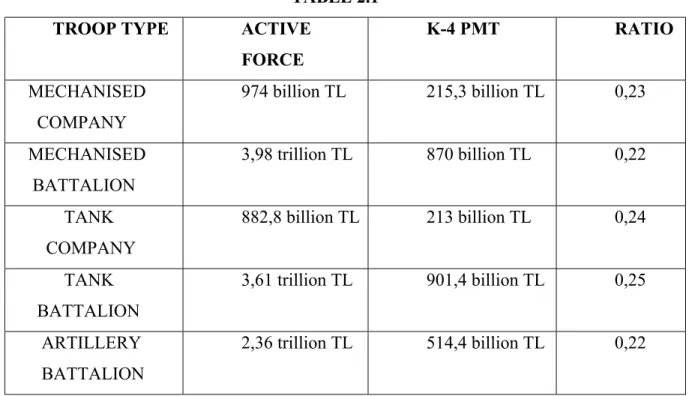
Real options can be applied to the combat readiness of the Turkish Armed Forces. Maintaining certain equipment at minimum cost improves efficiency in use of resources available for the military. Turkish Armed Forces can be classified in two categories: Readily deployable forces, and the forces that would be deployable after the declaration of war. Readily deployable forces are now at their full capacity and they can be deployed whenever it is necessary. They are equipped, mobilized, and manned. The other type of forces that would be deployable after the declaration of war, K-4 PMT5 as in military literature, are equipped, mobilised but unmanned. The equipment is kept under storage, but not mothballed and they are maintained to be used whenever they are needed.
A quick look at the annual costs of two systems can help us in differentiating them:
TABLE 2.1 TROOP TYPE ACTIVE
FORCE K-4 PMT RATIO MECHANISED COMPANY 974 billion TL 215,3 billion TL 0,23 MECHANISED BATTALION 3,98 trillion TL 870 billion TL 0,22 TANK COMPANY 882,8 billion TL 213 billion TL 0,24 TANK BATTALION 3,61 trillion TL 901,4 billion TL 0,25 ARTILLERY BATTALION 2,36 trillion TL 514,4 billion TL 0,22
Source: Uzun Süreli depolama Projesi,2001, Genel Kurmay Başkanlığı Kara Kuvvetleri Komutanlığı, Lojistik Daire Başkanlığı
16
If we compare at the annual costs of tank battalion in the active force and K-4 PMT, we will see the big difference between them. But the cost of K-4 PMT still seems very large. To understand the reason we should consider the maintenance function. Use it or not, 0,015% of a Tank is depreciated every day. The standard cost of a new tank is $7 million.
If we compute the annual straight line depreciation cost: $7 million*365*0,015=$383,000
If we use declining balance method in computing the yearly depreciation the result is $372,975.
The motor type of the tanks that we use as an example is AVDS-1790. It has a life span of 1200 hours. Use it or not, it has to be operated 200 hours in a year. So even if you do not use it for combat purposes it will complete its operational life in 6 years. K-4 PMT reduces the costs but you cannot lower them when limitations are reached.
The modernization of military technology and the need for a professional army have forced Turkish Army to make radical changes in the maintenance of its readiness level.
Mothballing is commonly used in the modern armies as a means of preserving military hardware. Tanks, ships, helicopters, and all kind of military equipment that are not needed now, are mothballed for a specific period in order to reduce their maintenance costs. Germany mothballs its vehicles and tanks in peacetime. Its tanks are kept under special depots with a certain humidity of 45%. Under this humidity, the motor oil is not dried up, and it is rustproof, and no periodical maintenance is needed. If Germany faces a threat, she can use these brand new tanks whenever she wants. If a tank is mothballed you do not need to operate it in order to keep it ready. As a result the annual maintenance costs can
17
be reduced. If we compare the maintenance costs of a tank division we get the following results:
TABLE 2.2
ACTIVE FORCES K-4 PMT AFTER
MOTHBALLED 3,61 trillion TL 0,9014 trillion TL 0,15 trillion TL Source: Uzun Süreli depolama Projesi,2001, Genel Kurmay Başkanlığı Kara Kuvvetleri Komutanlığı, Lojistik Daire Başkanlığı
Mothballing a tank division requires the construction of a depot that can provide 45% humidity. The cost for constructing such a depot is given below:
TABLE 2.3
COST OF CONSTRUCTION 1,85 trillion TL
COST OF UTILITIES 145 billion TL
INSTALLING FIRE EXTINGUISHER MECHANISM
765 billion TL INSTALLING INTERNAL SECURITY
SYSTEM
95 billion TL INSTALLING HEATING & A/C
SYSTEM
955 billion TL
TOTAL 3,8 trillion TL
Source: Uzun Süreli depolama Projesi,2001, Genel Kurmay Başkanlığı Kara Kuvvetleri Komutanlığı, Lojistik Daire Başkanlığı
In this study we will try to find out the thresholds of when to invest, mothball, scrap, or reactivate the tank division. we will denote the cost of mothballing by EM. In addition, once a division is mothballed, maintaining the
equipment requires a cost flow M. The mothballed division can be reactivated in the future at a further sunk cost R. Mothballing only makes sense if the maintenance cost M is less than the cost C of actual operation, and if the
18
reactivation cost R is less than the cost of fresh investment I; we will assume that these conditions meet our objective of determining the value of an operating project, the value of the opportunity to invest in such a project, and the decision rules for investment, mothballing, reactivation, and scrapping are affected by various costs like I, Em, M, and R .
Output prices are determining factors in evaluating mothballing parameters. But prices move randomly and can be represented as a Wiener process. A Wiener process-also called Brownian motion- is a continuous-time stochastic process with three important properties:
• The probability distribution for all future values of the process depends only on its current value, and is unaffected by past values of process or by any other information. As a result, the current value of the process is all one needs to make a best forecast of its future value.
• The Wiener process has independent increments. The probability distribution for the change in the process over any time interval is independent of any other time interval.
• The changes in the process over any finite interval of time are normally distributed, with a variance that increases linearly with the time interval.
A stochastic process is a variable that evolves over time randomly. The temperature in Ankara is an example; its variation through time is partly deterministic. It rises through out the day and falls at night. The price of ISE stock is another example; it fluctuates randomly. But there is a difference between the temperature in Ankara and the price of ISE stock; the temperature in Ankara is a stationary process. The statistical properties of this variable are constant over time. For example, although the expected temperature tomorrow may depend on today’s temperature, the expectation and variance of the temperature on March 1 of next year is largely independent of today’s temperature, and is equal to the expectation and variance of the temperature on
19
March 1 two years from now. The price of ISE stock on the other hand, is a non-stationary process. The price of a sock is on March 1 next year cannot be estimated from the price of the same price on this year’s March 1. When we look at the investment costs of the army we can realize that the prices change randomly. The investments costs of the defense system change due to the probability of war and mutual relations between the countries. You cannot estimate the next year’s price of a tank by looking at today’s price.
The Wiener process below can is a geometric Brownian motion. dV=αV dt + σV dz
where dz is the increment of a Wiener process. α is called the drift parameter, and σ is called the variance parameter. The change in V over any time interval t, is normally distributed, and has an expected value E(∆v) = α∆t and variance ε(∆x) = σ∆t. The equation implies that the current value of the project is known, but future values are lognormally distributed with a mean and variance that grows linearly with time. Thus although information arrives continuously, the future value of the project is always uncertain.
We will assume that the costs follow geometric Brownian motion. The Army must decide whether and when a tank division should be mothballed, taking into account the uncertainty over future prices. Intuition suggests that an idle army will purchase new equipment when demand conditions become sufficiently favorable, and an already invested army will abandon when they become sufficiently adverse. Starting from a state in which it does not have any kind of capital installed, the army will make the investment if the profit rises to a threshold PH. The army will mothball an operating project if the profit falls to
another threshold PM. Given a project in mothballs, the army will reactivate it if
the profit raises to yet a third threshold PR. Since the cost of reactivation is less than that of investing from scratch, we expect PR<PH. If instead the profit falls,
making reactivation sufficiently unlikely or a remote event, there is a fourth threshold PS at which the mothballed project will be scrapped altogether to save
20
Of course all these thresholds PH, PM, PR, and PS are endogenous. Even
more fundamentally, we must ask if the army will find it optimal to use the mothballing option at all. If the maintenance cost M is sufficiently high, or the reactivation cost R not sufficiently less than the full investment cost I, then the army might find it better to scrap an operating project directly if the price hits the lower threshold PL. So, we must determine endogenously whether mothballing is
beneficial for the army.
21
3. THE DECISION TO ENTER, EXIT, MOTHBALL, AND SCRAP
In the previous chapter we defined investment and methods used to evaluate the investment decision. Unlike the other methods, real options can take into account the possibility to delay, mothball, or abandon investment decisions. While evaluating an investment decision, the decision makers generally care about the net present value of the cash flows generated by the investment. This cash flow could sometimes be negative, and we assume that at those times the firm could suspend operation, and resume it later when the cash flow turned out to be positive.
The new vision of the Army Chief of Staff needs a much lighter and a more rapidly deployable army. In the new system, only a more professional, flexible, and effective army can meet the task of managing defense risks. The change in the new defense system requires downsizing in the army. Since the old system was formed on mass army structure in case of a downsizing the decision makers would face with the problem of surplus weapons, equipment, and vehicles.
If we consider the Army as a firm, in case of a downsizing she could not be able to use her resources at full capacity; there would be a surplus of resources, which would not be utilized. She would face with some alternatives about what to do with that surplus.
If the army decides to abandon, she would sell her resources for their scrap values and possibly make a loss, but she would never pay for operating costs. In case of a threat, if the professional army would not be able to secure the country, every citizen would be drafted for defense purposes since our freedom would be in danger. This requires quick training and armament of civilians. And when conditions require full capacity, she would need to reinvest and pay large amounts of money.
If the army decides to continue with the current position she would pay operating costs and the vehicles would depreciate without generating profits. Since only some of the armament would be used, the unused ones would rust literally, and she would loose them after a while. And in case of a threat she would not be able to
22
use them, and she would not have funds to reinvest since she continued to pay operating costs without using them.
Instead of abandoning, the army may choose to keep her defense ability alive by maintaining armament by mothballing but not actively using them. Mothball option incurs an ongoing maintenance cost, but saves the prospect of future reinvestment cost. If the army chooses mothballing, the armament are deactivated and kept in special storages, and in case of a need to use them, they are reactivated.
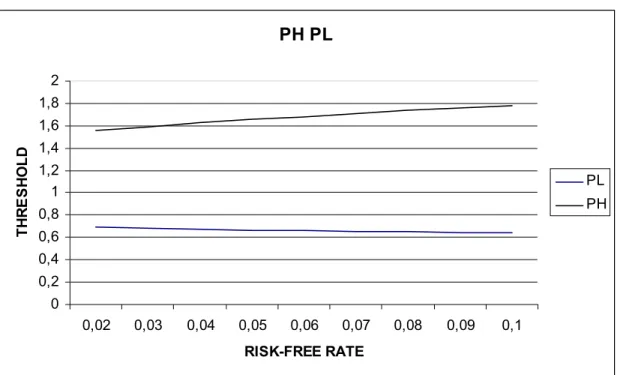
Dixit and Pindyck (1994) analyze a firm’s entry and exit decisions under uncertainty about the future expectations. They suggest that an idle firm will invest when demand conditions become sufficiently favorable, and an active firm will abandon when they become sufficiently adverse. The optimal strategy for investment and abandonment, or for holding or exercising the two options, will take the form of two threshold profits, PH and PL, with PH > PL. An idle firm will find it optimal to
remain idle as long as P, which denotes profit, remains below PH, and will invest as
soon as P reaches the threshold PH. An active firm will remain active as long as P
remains above PL, but it will abandon if P falls to PL. In the range of profits between
the thresholds PL and PH, the optimal policy is to continue with the status quo,
whether it is active or idle. If the firm had already invested it must consider the mothballing option if P decreases to another threshold of PM. If the firm has already chosen mothballing, it will reactivate if the profit rises to another threshold PR. Since the cost of reactivation is less than reinvesting PR<PH. If P falls down to the threshold PS, then mothballed project will be scrapped to save on maintenance costs and the firm will revert to the original idle state.
Above we mentioned five alternatives for a firm; • Stay idle,
• Abandon, • Mothball,
• Mothball to reactivate, • Mothball to scrap.
23
We will find out the thresholds, which will be used in evaluating the decision made about surplus weapons for the army.
3.1 THE BASIC MODEL FOR REAL OPTIONS
We will begin from the investment decision of an army and establish expressions for thresholds. The value of the army is a function of the exogenous state variable P, which denotes cost-savings, and of the discrete state variable that indicates whether the army has not currently invested (idle (0)) or has invested before (active (1)). Each army whether active or idle has an option; an idle army has the option to invest, and an active army has the option to abandon. To clarify this, we will change the notation slightly, letting V0 (P) denote the value of the option to invest (that is, the value of an idle army), and letting V1 (P) denote the value of an active army.
Between the prices (0, PH), an idle army remains idle and does not kill its
option to invest. Similarly, between the prices (PL.,∞), an active army remains
active, and does not kill its option to abandon.
Our starting point is a model developed by McDonald and Siegel (1985). They considered the following problem: At what point is it optimal to pay an investment cost I, in return for a project whose value is V, given that V follows geometric Brownian motion presented as;
dV = αV dt + σ V dz (3.1.1)
where dz is the increment of a Wiener process.
The equation implies that the current value of the project is known, but future values are lognormally distributed with a variance that grows linearly with the time horizon. Thus although information arrives over time, the future value of the project is always uncertain.
24
The army’s investment opportunity is equivalent to a call option – the right but not the obligation to invest. The decision to invest is to decide to exercise the option.
We will denote the value of investment opportunity by F (V). I want a rule that maximizes this value. Since the payoff from investing at time t is VT – I, we want to maximize its expected present value:
F (V) = max E ((VT – I) e- rT) (3.1.2)
where E denotes the expectation, T is the unknown future time, r is the discount rate, and the maximization is subject to equation (3.1.1) for V. We must also assume that α< r otherwise interpreting of (3.1.1) could be made indefinitely larger by choosing a larger T. Thus waiting longer would always be a better policy, and the optimum would not exist. We will use δ to denote r - α; where δ>0.
In the deterministic case, if the current V is given, the present value of the investment opportunity at time T is:
F (V) = (V eαT– I) e- rT) (3.1.3)
Suppose α ≤ 0 then V (t) will remain constant or fall over time, thus it is optimal to invest immediately if V>I, and never invest otherwise. Therefore the value of the option can be written as
F (V) = max (V-I, 0) (3.1.4)
If 0 < α < r then F (V) > 0 when V < I, since V will exceed I. Also, if V exceeds I, it may be better to wait rather than invest now. If we maximize F (V) in equation (3.1.3) with respect to T, the first order condition will be
25 This implies
T∗= max{1/ α log [r I / (r-α) V], 0} (3.1.6)
By setting T∗= 0, we see that one should invest immediately if V≥ V∗ where
V∗ = r I / r-α > I (3.1.7)
V∗ is the critical value at which it is optimal to invest. By substituting the equation (3.1.6) into equation (3.1.3), we obtain the valuation of the option for the deterministic case
F (V) = [α I / (r-α) ][(r-α) V / r I] r / α for V ≤ V∗ (3.1.8)
F (V) = V-I for V > V∗ (3.1.9)
In the stochastic case where the value of V is random, the problem becomes optimal stopping problem where one solves for the optimal investment to obtain a given V. For the values of V in which it is not optimal to invest the Bellman equation is
rF dt = E (dF) (3.1.10)
The equation above means that over a time interval dt, the total expected return on the investment opportunity, rF dt, is equal to its expected rate of capital appreciation.
We expand dF using Ito’s Lemma, and we use primes to denote derivatives, for example,
F’= dF / dV, F”=d2 F / dV2. Then
dF= F’ (V) dV +1/2 F” (V) (dV) 2
F` and F`` are first and second order derivatives of the function F. Substituting equation (3.1.1) for dV into this expression and noting that E (dz) =0 gives
26
E (dF) = αV F’ (V) dt + 1/2 σ2 V 2 F” (V) dt (3.1.11)
The Bellman equation becomes;
1/2 σ2 V 2 F” (V) + αV F’ (V) – rF = 0 (3.1.12)
In addition, F (V) must satisfy the following boundary conditions; F (0) = 0 (3.1.13)
This condition states that if V goes to zero, the value of the investment will be zero and no one will invest.
F (V∗) = V∗- I (3.1.14)
This condition arises from the observation that, upon investing the firm receives a net payoff V∗- I.
F’ (V∗) = 1 (3.1.15)
To find F (V), we must solve the partial differential equation (3.1.12) subject to the boundary conditions (3.1.13, 3.1.14, and 3.1.15). For a second order partial differential equation, the following is a particular solution that satisfies the boundary conditions.
F (V) = AVβ1 (3.1.16)
where A is a constant that is yet to be determined, and β1> 1 is a known constant whose value depends on the parameters σ, r, and δ of the differential equation.
The remaining boundary conditions (3.1.14, 3.1.15) can be used to solve for the remaining unknowns – the constant A, and the critical value V∗ at which it is
27
optimal to invest. By substituting (3.1.16) into (3.1.14, 3.1.15) and rearranging, it is found that
V∗= β1 I / β1-1 (3.1.17)
A= (V∗- I) / (V∗) β1 (3.1.18) A = (β1-1)β1-1 / [(β1)β1 Iβ1-1] (3.1.18)
Equations (3.1.16, 3.1.17, and 3.1.18) give the value of the investment opportunity and the optimal investment rule.
Since the second-order differential equation (3.1.12) is linear in the dependent variable F and its derivatives, its general solution can be expressed as a linear combination of any two independent solutions. If we try the function AVβ, we see by substitution that it satisfies the equation provided β is a root of the quadratic equation
1/2 σ2β(β-1) + (r-δ)β-r = 0 (3.1.19)
The roots are
β1 = 1/2- (r-δ) / σ2 + ((r−δ)÷σ2−0,5)2+2r÷σ2) > 1 and (3.1.20)
β2 = 1/2- (r-δ) / σ2 - ((r−δ)÷σ2−0,5)2+2r÷σ2) < 0 (3.1.21)
So the general solution to equation (3.1.12) can be written as F (V) = A1 Vβ1 + A2 Vβ2 (3.1.22)
where A1 and A2 are constants to be determined. The boundary condition (3.1.13) implies that A2 =0, leaving the solution (3.1.16).
28
3.2 VALUING THE PROJECT WITH NO OPERATING COSTS
We will assume that the cash-saving flow P of a project follows the geometric Brownian motion.
dP = αP dt + σ P dz (3.2.1)
The cash-saving flow P is perpetuity, and its expected value grows at the trend rate α. If future revenues are discounted at the rate µ, then the expected present value V of the project is just given by
V = P / (µ-α) (3.2.2)
This is the discounted cash flow valuation of an asset with growth rate α. Moreover V, which is a constant multiple of P, also follows a geometric Brownian motion with the same parameters α, and σ.
If we rewrite the equation (3.1.15) we will get
A1 (P) β1 = P/ δ - I (3.2.3)
Using the boundary conditions we obtain the value of A1 as;
A1 = (β1-1)β1-1 Iβ1-1 / (δ β1) β1 (3.2.4)
3.3 THE VALUE OF THE PROJECT UNDER OPERATING COST AND TEMPORARY SUSPENSION
P, which denotes cash saving, follows the geometric Brownian motion of equation, there is a correlation between the return of a portfolio and market. According to CAPM, the risk adjusted expected return of such portfolio is
29
where r is the risk-free rate, rM is the market risk. β is a known constant whose value depends on the parameters σ, r, and δ of the differential equation. Then, α, σ, µ, and δ = µ - α are all constants. For investment to occur, we need µ >α, and we will assume that this is indeed the case. The difference between risk adjusted return and return to V is δ = µ - α , and δ represents dividend yield. The total expected return would be dividend yield plus capital gain µ= α + δ. We will also assume that operation of the project entails a flow cost C, but that the operation can be temporarily and costlessly suspended when P falls below C, and costlessly resumed later if P rises above C. therefore at any instant the cash saving from this project is given by
π(P) = Max (P – C, 0) (3.3.2)
McDonald and Siegel (1985) pointed out another useful way to look at such a project. It gives the owner an infinite set of options. The option at time t, if exercised, means paying C to receive the P that prevails at that time. Since each option can only be exercised at its specified maturity, these are European call options. They also showed that the project could be valued by valuing each of these options.
In the region P<C, we have π(P) = 0. Therefore the general solution is just a linear combination of the two power solutions corresponding to the two roots;
V (P) = K1 Pβ1 + K2 Pβ2 (3.3.3)
where the constants K1 and K2 are to be determined. In the region P>C, we take another linear combination of the power solutions. P/δ is the discounted value of all future cash flows. It is a particular solution to the valuation of the project. If we subtract operational costs, the present value of operational cost at the discount rate r is C/r for infinitely lived assets. The particular problem becomes:
30
If we rearrange the formulas we can see that (P/δ - C/r) satisfies the equation. Therefore the general solution for P>C is
V (P) = K1 Pβ1 + K2 Pβ2 + P/δ - C/r (3.3.5)
In the region P<C, operation is suspended and the project yields no current cash saving. However there is a positive possibility that the process will at some future time move into the region P>C, when operation will resume and cash saving will accrue.
The constants in the solutions are determined using considerations that apply at the boundaries of the regions. If P becomes very small, the event of its rising above C becomes unlikely. The expected present value of future cash saving should then go to zero, and so should the value of the project. However with β2 negative, Pβ2 goes to ∞ as P goes to 0. Therefore the constant multiplying this term, K2, should be zero. When P becomes very large, the suspension option is unlikely to be exercised, so its value should be zero. Therefore the constant multiplying this term, K1, should be zero. This leaves us
V (P) = K1 Pβ1 if P<C (3.3.6)
V (P) = K2 Pβ2 + P/δ - C/r if P>C (3.3.7)
At P=C the two regions meet leaving us
K1 Cβ1 = K2 Cβ2 + C/δ - C/r (3.3.8)
β1K1 Cβ1-1 = β2K2 Cβ2-1 + 1/δ (3.3.9)
These are two linear equations in the unknowns K1 and K2; they readily yield the solution
31
K2 = C1-β2 / β1-β2 (β1 / r-β1-1 /δ) (3.3.11)
At the investment threshold PH, the army pays the investment cost I to exercise its investment option, giving up this asset value of V0 (PH) to get the live project which has value V1 (PH)
V0 (PH) = V1 (PH) – I (3.3.12)
V0’ (PH) = V1’ (PH) (3.3.13)
Likewise at the abandonment threshold PL, the army pays the abandonment cost E to exercise its abandonment option the conditions are
V1 (PL) = V0 (PL) – E (3.3.14)
V1’ (PL) = V0’ (PL) (3.3.15)
Using the conditions for V0 (P) and V1 (P) these conditions can be written as
A1 PHβ1 + B2 PHβ2 + PH/δ - C/r = I (3.3.16)
β1 A1 PHβ1-1 + β2B2 PHβ2-1 + 1/δ = 0 (3.3.17)
A1 PL β1 + B2 PLβ2 + PL/δ - C/r = -E (3.3.18)
β1 A1 PLβ1-1 + β2B2 PLβ2-1 + 1/δ = 0 (3.3.19)
These four equations determine the four unknowns – the thresholds PH, PL which are investment and abandonment thresholds, and the coefficients A1 and B2 in the option values. I is the investment cost and E is the abandonment cost.
3.4 THRESHOLDS IN THE MOTHBALLING OPTION
The army can be in the idle state over the cost interval (0, PH). Then its value is once again given by the equation:
32
V0 (P) = A1 Pβ1 (3.4.1)
where A1 is the constant to be determined. This is just the value of the option to invest. We have eliminated the term in the negative power β2 by using the fact that V0 (I) must go to zero as P goes to zero.
Similarly the active state can prevail over the interval (PM.,∞), with the value
of the army given by the equation:
V1 (P) = B2 P β2 + P/δ - C/r (3.4.2)
where the constant B2 remains to be determined. The first term is the value of the option to mothball. The other two terms are the expected present values of cash flows from continuing operations forever. The mothballing option derives its value from further possibilities of reactivation or scrapping.
The mothballed state can continue over some range of prices (PS, PR). Since
neither zero nor infinity is included in this range, we cannot eliminate either the positive or the negative power in the option value part of the solution. Therefore the value of the mothballed project is given by:
VM (P) = D1 Pβ1 + D2 Pβ2 - M/r (3.4.3)
where the constants D1, and D2 remain to be determined. The first term is the value of the option to reactivate the project. The second term is the value of the option to scrap the project and the last term is the capitalized maintenance cost, assuming that the project remains in the mothballed state forever.
Our investment threshold is PH meaning that if the project is to be activated it must have the exact value, and that value must be at least equal to the investment cost I. The equation is:
33
The equation above means that we should only invest if the cash saving is greater than zero after we subtracted the investment cost I.
If the project is already activated the mothballing threshold PM must be at least equal to the mothballing cost EM. The equation is:
V1 (PM) = VM (PM) - EM (3.4.5)
If the project is already mothballed the reactivation threshold PR, must be at least equal to the reactivation cost R The equation is:
VM (PR) = V1 (PR) – R (3.4.6)
And if we want to scrap an already mothballed project the threshold for scrapping PS must be at least equal to the scrapping cost. The equation is:
VM (PS) = V0 (PS) – ES (3.4.7)
And if we want to abandon a project the threshold for abandoning PL must be at least equal to the abandonment cost. The equation is:
V1 (PL) = V0 (PL) – E (3.4.8)
These equations determine the five thresholds PM, PH, PR, PS, PL and the option value coefficients A1, B2, D1, and D2.
We can use the interaction between the mothballing and reactivation to determine the limits on the range of the parameters where the mothballing option is used. Using the functional forms above, the four equations at these two thresholds become
-D1 PRβ1 + (B2 - D2) PRβ2 + PR / δ - (C-M) / r = R (3.4.9)
34
- D1 PMβ1 + (B2 - D2) PMβ2 + PM / δ - (C-M) / r = -EM (3.4.11)
-β1 D1 PMβ1-1 + β2(B2 - D2) PMβ2-1 + 1 / δ = 0 (3.4.12)
We can regard this as a system of four equations in four unknowns D1, (B2 -D2), PM, and PR, and solve it on its own. What we need to do is interpreting R as the cost of investment, EM as the cost of abandonment, and (C-M) as the cost of operation.
We can use the interaction between mothballing and scrapping to determine the limits on the range of the parameters where the mothballing option is used. For mothballing to be a part of the optimal strategy, we must have PM>PS. the equation sat these two thresholds are;
(D1 - A1) PSβ1 + D2 PSβ2 - M / r = ES (3.4.13)
β1(D1 – A1) PSβ1-1 + D2 PSβ2-1 = 0 (3.4.14)
-A1 PCβ1 + B2 PCβ2 + PC/δ - C/r = - (EM+ES) = -E (3.4.15)
35
4. THE DECISION TO INVEST AND TO STAY IDLE
The decision to invest can be given by various methods that we mentioned in the first chapter. Net present value is generally used in deciding whether to invest or not. But in the NPV rule you do not have a chance to make assumptions. You have to know exact cash outflows and inflows to compute the NPV of a project. In this chapter, we determine the thresholds, which will be used in evaluating the decision to invest in a project under uncertainty.
4.1. INVESTMENT AND ABONDONMENT THRESHOLDS
To invest in a project we look to get a higher return than the cost. There are two situations: the cash savings from the project, which is P, can be either smaller or greater than the outflow of the project, which is C. In the region P<C, the operation is suspended and the project yields no current cash saving. However there is positive probability that the price process will at some future time move into the region P>C, when operation will resume and cash savings will accrue. In the region P<C, the value of the project is just the expected present value of future cash savings.
In the region P>C, the expected value of the revenues grows at the rate α, and is discounted back at the appropriate risk-adjusted rate of return µ, so the expected discounted present value is P/(µ-α)=P/δ. The constant cost C is discounted at the riskless rate r, yielding a present value C/r.
K1Pβ1 if P<C (3.3.6)
V (P) =
K2Pβ2 + P/δ – C/r if P>C (3.3.7)
If we find out the point where P=C, we will be able to detect our investment threshold. The optimal strategy for investment and abandonment will take the form of two threshold prices, PH and PL, with PH > PL. An idle army will
36
find it optimal to remain idle as long as P remains below PH, and will invest as soon as P reaches the threshold PH. If the Army did not invest in military equipment we consider it idle. If economic conditions were the real determinants1 of the investment decision than the army would look at the future cash savings and invest if and only if the cash saving threshold rises above the PH. An active army will remain active as long as P remains above PL, but it will abandon if P falls to the threshold PL. If the Army has already invested, than to abandon it, it must wait for the cash saving threshold to decrease under PL. Otherwise it would not be optimal to abandon a cash saving investment. If the army wants to modernize her military equipment, she would compare the cash savings of the old and new system, and invest if the older investment cash saving lies below PL, and the new investment cash saving lies above PH. In the range between the thresholds PH and PL, the optimal policy is to continue with the current status, whether stay active or idle.
(0, PH) = Hold on your option to invest, stay idle. (PH,∞) = Exercise your option, invest.
(PH, PL) = Keep your position.
(PL,∞) = Hold on your option to abandon, stay active. (0, PL) = Exercise your option, abandon.
4.2 INVESTMENT AND ABANDONMENT THRESHOLDS FOR THE ARMY
TABLE 4.2
r Σ µ C I R EM ES M E 0.05 0.2 0.05 3.61 700 15 3.8 200 0.15 700 PH = 102.15 PL =41.7237
All the data in Table 4.2 are taken from the Land Forces Headquarters of the Turkish Army. Risk-free rate is r, standard deviation is σ, and risk-adjusted discount rate is µ. C is the operation cost, I is the investment cost for 100 tanks, R is the reactivating cost of mothballed tanks, EM is the mothballing cost, ES is the scrap value, M is the maintenance cost of mothballed tanks and E is the abandonment cost and they are all in trillions. All the findings below are found by using the formulas mentioned before. When I examine the effect of investment cost I only changed the value of investment cost and hold everything else constant. Likewise when I examine the effect of standard deviation I only changed the values for standard deviation living everything else constant
4.2.1. THE EFFECT OF INVESTMENT COST ON THE INVESTMENT AND ABANDONMENT THRESHOLDS
TABLE 4.2.1 I PL PH 2 1,52 1,65 3 1,66 1,84 4 1,79 2,02 5 1,92 2,19 6 2,05 2,36 7 2,16 2,52 8 2,27 2,67 9 2,38 2,83 10 2,49 2,98
If we increase the investment cost, we can see that both the investment threshold PH and the abandonment threshold PL also increase as we expect. If the investment cost increases from 2 to 3, the abandonment threshold increases from 1.52 to 1.66, and the abandonment threshold increases from 1.65 to 1.84. If the cost of investment increases we expect higher return so investment threshold