FAST AND ACCURATE ANALYSIS OF LARGE META-MATERIAL STRUCTURES USING THE MULTILEVEL FAST MULTIPOLE ALGORITHM
L. G¨urel, ¨O. Erg¨ul, A. ¨Unal, and T. Malas†
Computational Electromagnetics Research Center (BiLCEM) Bilkent University
TR-06800, Bilkent, Ankara, Turkey
Abstract—We report fast and accurate simulations of metamaterial structures constructed with large numbers of unit cells containing split-ring resonators and thin wires. Scattering problems involving various metamaterial walls are formulated rigorously using the electric-field integral equation, discretized with the Rao-Wilton-Glisson basis functions. Resulting dense matrix equations are solved iteratively, where the matrix-vector multiplications are performed efficiently with the multilevel fast multipole algorithm. For rapid solutions at resonance frequencies, convergence of the iterations is accelerated by using robust preconditioning techniques, such as the sparse-approximate-inverse preconditioner. Without resorting to homogenization approximations and periodicity assumptions, we are able to obtain accurate solutions of realistic metamaterial problems discretized with millions of unknowns.
1. INTRODUCTION
Metamaterials are artificial structures that are constructed by periodically arranging unit cells, such as split-ring resonators (SRRs) and thin wires. Due to the resonant nature of the cells, electromagnetic properties of the host medium, i.e., permittivity, permeability, or both, can effectively become negative for some frequencies. Although metamaterials were theoretically studied more than 40 years ago [1], their actual realizations were achieved recently [2–4]. Since then,
Corresponding author: ¨O. Erg¨ul ([email protected]).
† L. G¨urel, ¨O. Erg¨ul, and T. Malas are also with Department of Electrical and Electronics Engineering, Bilkent University, TR-06800, Bilkent, Ankara, Turkey. A. ¨Unal is now with Meteksan Defence, TR-06800, Bilkent, Ankara, Turkey.
there have been many studies on how to further enhance the desired electromagnetic properties and improve the practicability of metamaterials [5–7]. (See also [8] for an extensive discussion on metamaterials and a wide list of references.) Due to these efforts, metamaterials have been utilized in various applications [9], such as sub-wavelength focusing [10, 11], cloaking [12], and designing improved antennas [13, 14].
In this paper, we present fast and accurate analysis of large and complicated metamaterial structures involving SRRs and thin wires. In order to mimic the actual metamaterial structures used in real life, we consider the solution of hundreds and even thousands of unit cells at a time, as opposed to a few unit cells or infinitely periodic patterns that can be analyzed via the solution of a single unit cell. Without using any homogenization approximations, scattering problems involving three-dimensional metamaterials are rigorously formulated using the electric-field integral equation (EFIE) [15]. Conductor surfaces are modeled by perfectly conducting sheets with zero thicknesses. For accurate numerical solutions, both EFIE and the surfaces of the metamaterial structures are discretized simultaneously with small planar triangles, on which the Rao-Wilton-Glisson [16] basis functions are defined. The resulting dense matrix equations are solved iteratively, where the matrix-vector multiplications are performed efficiently with the multilevel fast multipole algorithm (MLFMA) [17]. Solutions of realistic metamaterials involving large numbers of unit cells are further accelerated with the parallelization of MLFMA [18, 19]. Since the resonant nature of metamaterials inhibits a rapid convergence of the iterations, we also employ robust preconditioning techniques, such as the sparse-approximate-inverse preconditioner [20], to reduce the number of iterations.
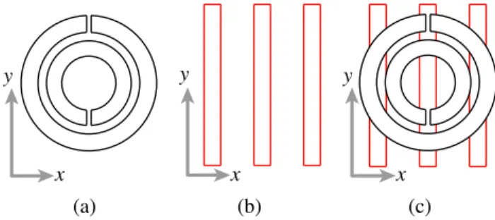
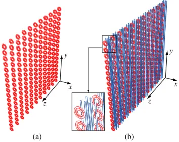
Figure 1 presents the unit cells that are used to construct the metamaterial structures investigated in this study. A single SRR, which is depicted in Figure 1(a), has dimensions in the order of microns. The smaller ring has an inner radius of 43 µm and an outer radius of 67.2 µm; the larger ring has an inner radius of 80.7 µm and an outer radius of 107.5 µm; and the gap width is 7.2 µm. With these dimensions, the SRR resonates at about 100 GHz, when it is located in a medium with a relative permittivity of 4.8 [6]. Around the resonance frequency, the SRR stimulates negative effective permeability in the medium. Dimensions of the thin wires depicted in Figure 1(b) are compatible with the dimensions of the SRRs and they exhibit negative effective permittivity in a wide range of frequencies, including 100 GHz. Finally, as depicted in Figure 1(c), we also consider composite metamaterials (CMMs) by combining SRRs and
y x y x y x (a) (b) (c)
Figure 1. Unit cells that are used to construct various metamaterial walls: (a) SRR, (b) thin wires, and (c) a combination of SRR and thin wires. y x y x y x (a) (b) (c)
Figure 2. Discretization (triangulation) of the unit cells in Figure 1. thin wires in the same medium to obtain a double-negative property. Discretizations of the unit cells are presented in Figure 2, where we use optimal numbers of planar triangles, i.e., we minimize the numbers of triangles for the efficiency of the simulations, while the triangles are sufficiently small to discretize the geometries and the surface currents accurately.
The rest of the paper is organized as follows. In Section 2, we present fast and accurate solutions of metamaterial problems using MLFMA. Then, Section 3 investigates the acceleration of the iterative solutions by using robust preconditioning techniques. Construction of metamaterial walls is detailed in Section 4, followed by our numerical results in Section 5 and concluding remarks in Section 6.
2. MLFMA SOLUTIONS OF METAMATERIAL PROBLEMS FORMULATED WITH EFIE
For perfectly-conducting objects, EFIE can be derived from the boundary condition for the tangential electric field on the surface (in
phasor notation with the e−iωt convention) as [15] ˆt · ikη Z S dr0 · J(r0) + 1 k2∇ 0· J(r0)∇ ¸ g(r, r0) = −ˆt · Ei(r) (1)
by expressing the scattered electric field in terms of the induced (unknown) surface current J(r). In (1), ˆt is any tangential unit vector on the surface, Ei(r) is the incident electric field due to external
sources, η =pµ/² is the impedance of the host medium, k = ω√µ² =
2π/λ is the wavenumber, and
g(r, r0) = eikR 4πR ³ R = |r − r0| ´ (2) denotes the homogenous-space Green’s function. Through the discretization of EFIE for the numerical solution of metamaterial problems, we obtain N × N dense matrix equations in the form of
N
X
n=1
Zmnan= vm, m = 1, ..., N, (3)
where the matrix elements and the elements of the excitation vector are derived as Zmn = ikη Z Sm drtm(r) · Z Sn dr0g(r, r0)bn(r0) +iη k Z Sm drtm(r) · Z Sn dr0∇0· bn(r0)∇g(r, r0) (4) and vm= − Z Sm drtm(r) · Ei(r), (5)
respectively. In (4) and (5), Sm and Sn are the spatial supports
of the mth testing function tm(r) and the nth basis function bn(r),
respectively. We use a Galerkin scheme and choose the basis and testing functions as Rao-Wilton-Glisson functions defined on planar triangles.
The matrix equation in (3) is solved iteratively, where the matrix-vector multiplications are accelerated by MLFMA. For an N ×N dense matrix equation, MLFMA reduces the complexity of the matrix-vector multiplications from O(N2) to O(N log N ). The fundamental idea in MLFMA is to replace the interactions of the basis and testing
functions with the interactions of clusters in a multilevel scheme. First, a tree structure with L = O(log N ) levels is constructed by including the metamaterial object in a cubic box and recursively dividing the computational domain into clusters. Then, cluster-to-cluster interactions are performed in different levels (from l = 1 to
l = L) efficiently using the factorization and diagonalization of the
Green’s function, which are valid only for the clusters that are far from each other [21]. In general, MLFMA splits the matrix-vector multiplications as
¯
Z · x = ¯ZN F · x + ¯ZF F · x, (6)
where the near-field interactions denoted by ¯ZN F are calculated
directly and stored in the memory, while the far-field interactions denoted by ¯ZF F are computed approximately via three main
stages, i.e., aggregation, translation, and disaggregation [17]. The preconditioners to be discussed in Section 3 are utilizing the near-field part of this splitting.
2.1. Aggregation
In the aggregation stage, radiated fields of the clusters are calculated from the bottom of the tree structure to the highest level (l = L). In the lowest level, the radiation pattern of a cluster C at a reference point rC can be calculated as
FC(rC, k) =X
n∈C
fn(rC, k)xn, (7)
where k = kˆk, fn represents the radiation pattern of the nth basis function inside the cluster, and xn is the coefficient provided by the iterative solver. In (7), radiation patterns FC and f
n have only θ and
φ components, and they are functions of the angular direction ˆk. For
a cluster C in a level l > 1, the radiation pattern can be obtained similarly as FC(rC, k) = X C0∈sub{C} exp£ik · (rC − rC0) ¤ FC0(rC0, k), (8)
where sub{C} represents the sub-clusters of C.
In our MLFMA implementations, radiation patterns are sampled uniformly in the φ direction, while we use the Gauss-Legendre quadrature in the θ direction [21]. There are a total of Sl = (Tl +
1) × (2Tl+ 2) samples required for each cluster in level l, where Tl is the truncation number. Using the excess bandwidth formula,
Tl≈ 1.73kal+ 2.16(d0)2/3(kal)1/3, (9)
where alis the cluster size, and d0is the desired digits of accuracy [22].
Since the sampling rate depends on the cluster size as measured by the wavelength (kal ∝ 2πal/λ), we use local Lagrange interpolation
to match the different sampling rates of the consecutive levels [23]. Complexity of the aggregation stage is O(N ) for each level.
2.2. Translation
In the translation stage of MLFMA, radiated fields of the clusters are translated into incoming fields for some other clusters. The incoming field to the center of a cluster C (due to translations) is calculated as
GC(rC, k) = X
C0∈f ar{C}
α(rC− rC0, k)FC
0
(rC0, k), (10)
where f ar{C} represents the clusters in the far-field list of C, and
α(rC − rC0, k) is the diagonal translation operator. For each cluster
in any level, there are O(1) clusters (in the same level) to translate the radiated field to. Therefore, the complexity of the translation stage is O(N ) per level. In addition, using cubic (identical) clusters, the number of different translation operators is O(1), independent of the level, due to the symmetry [24]. We use optimized interpolation methods to calculate these operators in O(N ) time during the setup stage, i.e., before the iterations [25].
2.3. Disaggregation
In the disaggregation stage, the total incoming fields at the centers of the clusters are calculated from the top of the tree structure to the lowest level. For a cluster C in level l < L, the total incoming field is calculated as
GCT(rC, k) = GC(rC, k)+exp£ik·(rC−rP {C})¤GP {C}T (rP {C}, k), (11)
where GC is the incoming field due to translations, and P {C} rep-resents the super-cluster (parent) of C. Following the disaggregation operations in the lowest level, incoming fields are received by the test-ing functions via an angular integration as
I =
Z
where gm represents the receiving pattern of the mth testing function inside a cluster C in the lowest level. Complexity of the disaggregation stage is also O(N ) per level.
In MLFMA, weights for the angular integrations in (12) are introduced in the translation stage since we use transpose interpolation (anterpolation) during the disaggregation to decimate the fields [26]. Consider the interaction of the nth basis and the mth testing functions via a translation in level l 6= 1. Then, the corresponding matrix element can be written as
Zmn∝
Z
d2k gˆ m(rC, k) · Gn(rC, k), (13)
where Gn is the incoming field due to the nth basis function‡. Since
Tl> T1 for l > 1, the sampling rate for Gn is larger than the sampling
rate for gm. An accurate way to calculate (13) could be to interpolate gm and to perform the numerical integration in the fine grid, i.e.,
Zmn∝ Sl X s=1 Γ1→l © gm ª [s]Gn[s]Wl[s], (14)
where Γ1→lis an interpolator from level 1 to l, while Wlrepresents the
integration weights for level l. However, the procedure in (14) is not appropriate for MLFMA, which involves a top-down disaggregation scheme. Therefore, without sacrificing accuracy, we perform the integration in the coarse grid as
Zmn∝ S1 X s=1 gm[s]ΓTl→1 © GnWl ª [s] (15)
by anterpolating Gnusing the transpose of the interpolator. We note
that the weights related to level l also need to be anterpolated, and it is appropriate to introduce them during the translations.
2.4. Power Transmission
After finding the coefficients an in (3), we calculate the near-zone
electric and magnetic fields as Et(r) = Ei(r) +ikη N X n=1 Z Sn dr0 · bn(r0) +k12∇0· bn(r0)∇ ¸ g(r, r0)an (16)
‡ Equation (13) represents the calculation of a single interaction in MLFMA. However, this expression is not used explicitly, because the interactions are actually calculated in a group-by-group manner.
and Ht(r) = Hi(r) + N X n=1 Z Sn dr0bn(r0) × ∇0g(r, r0)an, (17)
respectively, where Hiis the incident magnetic field. Then, the average
power density is evaluated as Ptav(r) =Pt(r)®= 1 2Re n Et(r) ×£Ht(r)¤∗ o . (18)
Finally, we define the power transmission at an observation point r as
T (r) = |P t av(r)| |Pi av(r)| , (19) where Piav = 1 2Re n Ei(r) ×£Hi(r)¤∗ o (20) is the average incident power density. In Sections 4 and 5, we will present power-transmission results in a decibel (dB) scale, defined as
TdB(r) = 10 log{T (r)}. (21)
Note that TdB(r) can take values greater than 0 dB since it is a
point-wise function.
3. ITERATIVE SOLUTIONS AND PRECONDITIONING MLFMA provides efficient matrix-vector multiplications by reducing the complexity from O(N2) to O(N log N ). However, efficiency
of the solutions also depends on the number of iterations and thus the conditioning of the matrix equations. Unfortunately, matrix equations obtained from EFIE have unfavorable conditioning characteristics, such as high indefiniteness and near singularity [27, 28]. For metamaterial problems, it can be more difficult to achieve a rapid convergence, due to the resonances of these structures. Because reducing the number of iterations is extremely important, we investigate and compare the convergences provided by various iterative algorithms. In general, the least-squares-QR [29] and the generalized-minimal-residual [20] algorithms provide improved convergence rates compared to other Krylov subspace algorithms for the solution of
problems formulated with EFIE [30]. On the other hand, for difficult problems involving large metamaterial structures, a robust solver alone may not be sufficient. Therefore, we also consider effective preconditioning techniques to reduce the number of iterations and obtain efficient solutions.
Preconditioning refers to transforming a matrix equation into another, but equivalent one with more favorable conditioning characteristics. In forward-type preconditioning, an easily invertible matrix ¯M, which approximates ¯Z in some sense, is selected. Thus, instead of the original matrix equation in (3), we solve a transformed equation in the form of
¯
M−1· ¯Z · a = ¯M−1· v. (22) Since ¯M approximates ¯Z, the product ¯M−1· ¯Z should approximate the
identity matrix, which may lead to a faster convergence with fewer iterations. In backward-type preconditioning, however, ¯M directly approximates the inverse of ¯Z, and the preconditioned matrix equation can be written as
¯
M · ¯Z · a = ¯M · v. (23)
Among various preconditioning techniques, the incomplete-LU preconditioner [31] is a forward-type preconditioner, which is commonly used to accelerate the solutions obtained with sequential implementations of MLFMA. In particular, “the incomplete-LU preconditioner with threshold” [28] is highly successful for EFIE. In parallel implementations, however, block-diagonal and sparse-approximate-inverse preconditioners are preferred over incomplete-LU-type preconditioners, due to their efficient parallelizations [32, 40].
The block-diagonal preconditioner is obtained by retaining the self interactions of the lowest-level clusters of the MLFMA tree. Due to its simplicity and favorable computing cost, this preconditioner is commonly used for the MLFMA solutions of second-kind integral equations, such as the magnetic-field integral equation and the combined-field integral equation [17]. Although it usually has an adverse effect on the convergence of EFIE [33, 34], the block-diagonal preconditioner may also accelerate the iterative solutions of metamaterial problems formulated with EFIE [35]. Nevertheless, we observe that the block-diagonal preconditioner is insufficient to improve the convergence at the resonance frequencies of the metamaterials. For such frequencies, sparse-approximate-inverse preconditioner provides more efficient solutions by significantly reducing the number of iterations, when compared to solutions without a preconditioner and with a block-diagonal preconditioner.
4. METAMATERIAL STRUCTURES
In this section, we briefly describe the construction of various metamaterial walls with SRRs and thin wires.
4.1. Split-ring Resonators
The SRR structure shown in Figure 1(a) exhibits a magnetic resonance [36] at about 100 GHz, when it is excited appropriately by electromagnetic waves. At the resonance frequency, the electromagnetic response of the SRR changes significantly. Even a single SRR is able to block the transmission of the waves, which can be observed as a shadowing effect. This unusual behavior around the resonance frequency can be explained with the induced negative effective permeability in the medium. Due to the complex effective wavenumber, the propagating power decays rapidly in the transmission region behind the SRR.
4.2. Thin Wires
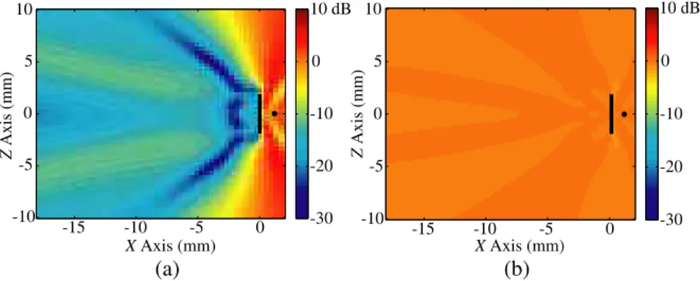
It is a well-known fact that periodical arrangements of thin wires can be used to block the electromagnetic waves, if the spacing between the wires is small compared to the wavelength and if the wires are aligned parallel to the electric field of the incident wave. As opposed to SRRs, the shadowing effect can be obtained with thin wires over a wide range of frequencies. This well-known shielding property can also be explained as the induction of negative effective permittivity in the medium [37]. As an example, Figure 3 presents the transmission results for an array of thin wires located on the x = 0 plane. The array is illuminated by a Hertzian dipole located to the right of the array and oriented in the y direction. We calculate the power transmission defined in (21) at various points on the y = 0 plane. In Figure 3(a), the thin wires lie along the y axis, and they are parallel to the dominant component of the incoming electric field. For this configuration, the effective permittivity becomes negative, and the power transmitted through the array is relatively low. In Figure 3(b), however, the array is rotated, and the incident electric field is mostly perpendicular to the thin wires. In this case, the thin-wire array becomes transparent, and the power transmission to the left of the array is close to 0 dB, corresponding to unity. Note that the x > 0 region on the y = 0 plane is also plotted so that the configuration of the thin wires and the dipole can be clearly seen, even though this region is not really the transmission region. Indeed, the high values of transmission in this region in Figure 3(a) correspond to power reflection.
Z Axis (mm) X Axis (mm) -15 -10 -5 0 -30 -20 -10 0 10 dB 10 5 0 -5 -10 (a) Z Axis (mm) X Axis (mm) -15 -10 -5 0 -30 -20 -10 0 10 dB 10 5 0 -5 -10 (b)
Figure 3. Power transmission (in dB scale) for a thin-wire wall illuminated by a Hertzian dipole, when the thin wires are (a) parallel and (b) perpendicular to the dominant electric-field polarization. 4.3. Composite Metamaterials
CMMs are constructed by carefully arranging SRRs and thin wires in the same medium. This way, the desired properties of the SRRs and thin wires can be combined, i.e., both effective permittivity and effective permeability can be simultaneously negative for some frequencies [2]. When the SRRs do not resonate, CMM structures are opaque due to the negative effective permittivity induced by the thin wires. At the resonance frequencies of SRRs, however, CMMs are unexpectedly transparent, which can be explained by the induced double negativity [38, 39].
4.4. Metamaterial Walls
We construct metamaterial walls by periodically arranging hundreds of SRRs and/or thin wires. As an example, Figure 4(a) depicts an 18 × 11 SRR array (1-layer wall) located at x = 0. The SRRs lie on planes perpendicular to the z axis, while the periodicity of the unit cells is 262.7 µm and 450 µm in the y and z directions, respectively. For multilayer walls, periodicity in the x direction is also selected as 262.7 µm. By combining this SRR array with thin wires, a CMM wall is constructed, as depicted in Figure 4(b). Among various possible arrangements of thin wires, we follow the strategies detailed in [6] and depicted in the inset of Figure 4(b), where two rows of thin wires can be seen between two consecutive SRR rows in the z direction.
z y x z y x (a) (b)
Figure 4. (a) 1-layer SRR wall involving 18 × 11 SRRs. (b) 1-layer CMM wall involving 18 × 11 SRRs combined with thin wires.
5. RESULTS
Figure 5 presents the power transmission results for 1-layer SRR, thin-wire, and CMM walls located at x = 0. The power transmission defined in (21) is calculated at various points on the z = 0 plane at 90 GHz, 95 GHz, 100 GHz, and 105 GHz. The excitation is a Hertzian dipole oriented in the y direction and located at x = 1.2 mm, as is also indicated by dots in the plots. Our observations are as follows:
(i) At 90 GHz and 95 GHz, the power transmission to the left of the SRR wall is almost unity (0 dB). At 100 GHz, however, the transmission drops drastically, and a shadowing effect is observed. At this frequency, the SRR wall is opaque, due to the negative effective permeability stimulated in the medium. The wall becomes transparent again at 105 GHz, although the transmitted power is less than 0 dB.
(ii) Different from the SRR wall, the thin-wire structure is opaque at all four frequencies as a result of the negative effective permittivity induced in the medium. This is achieved by properly aligning the thin wires, as explained in Section 4. Although there are some variations, the power transmission is generally less than −10 dB to the left of the wall.
(iii) The CMM structure constructed by combining the SRR and thin-wire walls is opaque at 90 GHz and 95 GHz. At these frequencies,
X Axis (mm) -15 -10 -5 0 X Axis (mm) -15 -10 -5 0 Y Axis (mm) 10 5 0 -5 X Axis (mm) -15 -10 -5 0 -10 Y Axis (mm) 10 5 0 -5 -10 Y Axis (mm) 10 5 0 -5 -10 Y Axis (mm) 10 5 0 -5 -10 -30 -20 -10 0 10 dB -30 -20 -10 0 10 dB -30 -20 -10 0 10 dB -30 -20 -10 0 10 dB 90 GHz 95 GHz 100 GHz 105 GHz CMM TW SRR
Figure 5. Power transmission (in dB scale) for 1-layer SRR [Figure 4(a)], thin-wire, and CMM [Figure 4(b)] walls at 90 GHz, 95 GHz, 100 GHz, and 105 GHz. Power transmission, as defined in Equation (21), is calculated and plotted on the z = 0 plane. A y-directed Hertzian dipole is radiating from x = 1.2 mm.
the transmission property of the CMM is dominated by the negative effective permittivity dictated by the thin wires. At 100 GHz, however, the structure becomes transparent, and we observe a relatively high power transmission to the left of the array. This unusual behavior of the CMM is a result of double negativity; since the SRRs resonate at 100 GHz, both effective permittivity and permeability of the medium become negative at this frequency. Then, the CMM wall is transparent even though its components, i.e., SRR and thin-wire walls, are opaque. The transparency of the composite structure tapers down at 105 GHz.
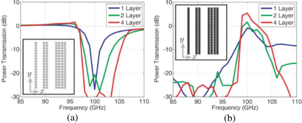
For quantitative information, Figure 6 presents the power transmission (at x = −1.2 mm) for various SRR and CMM walls as a function of frequency. In addition to 1-layer walls considered in the previous example, we also investigate 2-layer and 4-layer walls, as depicted in the insets of Figure 6. In Figure 6(a), we observe that the power transmission through the SRR walls drops significantly around the resonance frequency (100 GHz). This computational observation agrees remarkably well with the experimental results, e.g., Figure 4 in [6]. Furthermore, increasing the number of layers widens the frequency band for the shadowing effect; this property is also verified by measurement results presented in Figure 3 of [6]. Figure 6(b) shows that the power transmission through the CMM structures is maximized at 100 GHz, and increasing the number of layers improves the quality of the resonance effect. For the 4-layer CMM structure, transparency is achieved around 100 GHz, and the structure becomes opaque outside of the pass band around 100 GHz. Experimental results validating this phenomenon are available in the literature. Most notably, Figure 5 in [6] reports exactly the same pass band as Figure 6(b) since similar configurations are employed for both measurements in [6] and the computations here.
All results presented in Figures 5 and 6 are computed according to Equations (19) and (21). Hence, we label them as “power transmission.” Nevertheless, these results can also be interpreted as radiation and scattering results. This is because what is defined as power transmission is directly related to the total fields radiated by
(a) (b)
Figure 6. Power transmission (at x = −1.2 mm) for 1-layer, 2-layer, and 4-layer SRR and CMM walls as a function frequency: (a) SRR walls exhibit a stop band around 100 GHz. (b) CMM walls exhibit a pass band around 100 GHz.
the dipole and scattered by the metamaterial structure. Since this quantity is computed and plotted point-wise, as opposed to the total power, it can take on values higher than 0 dB; this does not contradict with the conservation of power.
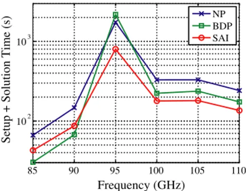
Figure 7 presents the processing time for the iterative solution of the 18×11×4 SRR wall discretized with 64,944 unknowns. The scattering problem is solved by using a generalized-minimal-residual algorithm accelerated with MLFMA parallelized into 8 processes [18, 19]. In addition to the no-preconditioner case, we employ block-diagonal and sparse-approximate-inverse preconditioners to reduce the number of iterations. Figure 7 depicts the processing time required for each case as a function of frequency. For a fair comparison, we include the setup time required by the preconditioners, together with the solution time. Without using a preconditioner, the processing time is less than 400 seconds at all frequencies, except for 95 GHz. Due to a numerical resonance, the processing time increases to 1700 seconds at 95 GHz. Using a block-diagonal preconditioner, the processing time is reduced at ordinary frequencies, while the solution at 95 GHz is even further decelerated, compared to the no-preconditioner case. On the other hand, using a sparse-approximate-inverse preconditioner with a threshold parameter of 0.05 [20], the solution is accelerated at all frequencies, including the resonance frequency, again compared to the no-preconditioner case. The processing time is reduced to 800 seconds at 95 GHz, corresponding to less than half the time
85 90 95 100 105 110
102
103
Frequency (GHz)
Setup + Solution Time (s)
NP BDP SAI
Figure 7. Processing time including the iterative solution and the setup of the preconditioner for the 18×11×4 SRR wall. “NP” represents the no-preconditioner case, while “BDP” and “SAI” represent the solutions accelerated with the block-diagonal preconditioner and the sparse-approximate-inverse preconditioner, respectively.
X Axis (mm) -15 -10 -5 0 Z Axis (mm) 10 5 0 -5 -10 -30 -20 -10 0 10 dB 110 GHz 100 GHz 85 GHz -30 -20 -10 0 10 dB -30 -20 -10 0 10 dB Z Axis (mm) 10 5 0 -5 -10 Z Axis (mm) 10 5 0 -5 -10 Z Axis (mm) 10 5 0 -5 -10 -30 -20 -10 0 10 dB 110 GHz 100 GHz 85 GHz -30 -20 -10 0 10 dB -30 -20 -10 0 10 dB Z Axis (mm) 10 5 0 -5 -10 Z Axis (mm) 10 5 0 -5 -10 X Axis (mm) -15 -10 -5 0 (a) (b)
Figure 8. Power transmission results (in dB scale) for a large SRR wall involving 51×29×20 SRRs on (a) y = 0 and (b) z = 0 planes. The results are obtained by solving a 2,425,560-unknown problem at several frequencies; solutions for 85 GHz, 100 GHz, and 110 GHz are shown here.
required without preconditioning. The gain obtained by using the sparse-approximate-inverse preconditioner is more significant for larger metamaterial problems.
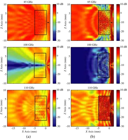
Finally, Figure 8 presents the transmission results for a large SRR wall involving 51×29×20 SRRs. The scattering problem is discretized with 2,425,560 unknowns and solved by using MLFMA parallelized into 64 processes [18, 19]. Figures 8(a) and 8(b) present the power
transmission on the y = 0 and z = 0 planes, respectively, when the wall is illuminated by a Hertzian dipole at 85 GHz, 100 GHz, and 110 GHz. The area occupied by the wall is indicated with the black frames in the plots. Similar to previous examples, SRRs are oriented perpendicular to the z direction, while the splits are along the y direction. In addition to a deep shadowing effect at 100 GHz, we observe that the low-transmission region has different shapes on the two planes. 6. CONCLUSION
We present accurate and efficient solutions of large metamaterial problems using a sophisticated simulation environment based on integral-equation formulations, iterative solutions, preconditioners, MLFMA, and parallel computing. Without using any homogenization approximations and assumptions of infinitely large periodic structures, we accurately calculate the power transmission through various metamaterial walls, including a 51×29×20 SRR array discretized with 2,425,560 unknowns. Computational results agree well with the experimental discoveries reported in the literature.
ACKNOWLEDGMENT
This work was supported by the Turkish Academy of Sciences in the framework of the Young Scientist Award Program (LG/TUBA-GEBIP/2002-1-12), by the Scientific and Technical Research Council of Turkey (TUBITAK) under Research Grants 105E172 and 107E136, and by contracts from ASELSAN and SSM.
REFERENCES
1. Veselago, V. G., “The electrodynamics of substances with simultaneously negative values of ² and µ,” Sov. Phys. Usp., Vol. 47, 509–514, Jan.–Feb. 1968.
2. Smith, D. R., W. J. Padilla, D. C. Vier, S. C. Nemat-Nasser, and S. Schultz, “Composite medium with simultaneously negative permeability and permittivity,” Phys. Rev. Lett., Vol. 84, 4184– 4187, May 2000.
3. Shelby, R. A., D. R. Smith, S. C. Nemat-Nasser, and S. Schultz, “Microwave transmission through a two-dimensional, isotropic, left-handed metamaterial,” Appl. Phys. Lett., Vol. 78, 489–491, Jan. 2001.
4. Shelby, R. A., D. R. Smith, and S. Schultz, “Experimental verification of a negative index of refraction,” Science, Vol. 292, 77–79, Apr. 2001.
5. Moss, C. D., T. M. Gregorczyk, Y. Zhang, and J. A. Kong, “Numerical studies of left handed metamaterials,” Progress In
Electromagnetics Research, PIER 35, 315–334, 2002.
6. Gokkavas, M., K. G¨uven, I. Bulu, K. Aydın, R. S. Penciu, M. Kafesaki, C. M. Soukoulis, and E. ¨Ozbay, “Experimental demonstration of a left-handed metamaterial operating at 100 GHz,” Phys. Rev. B, Vol. 73, No. 19, 193103-1–193103-4, May 2006.
7. Eleftheriades, G. V. and K. G. Balmain, Eds., Negative-Refraction
Metamaterials: Fundamental Principles and Applications,
Wiley-IEEE, New Jersey, 2005.
8. Engheta, N. and R. W. Ziolkowski, “A positive future for double-negative metamaterials,” IEEE Trans. Microw. Theory Tech., Vol. 53, No. 4, 1535–1556, Apr. 2005.
9. Chen, H., B. I. Wu, and J. A. Kong, “Review of electromagnetic theory in left-handed materials,” Journal of Electromagnetic
Waves and Applications, Vol. 20, No. 15, 2137–2151, 2006.
10. Grbic, A. and G. V. Eleftheriades, “Overcoming the diffraction limit with a planar left-handed transmission-line lens,” Phys. Rev.
Lett., Vol. 92, No. 11, 117403-1–117403-4, Mar. 2004.
11. Aydın, K., I. Bulu, and E. ¨Ozbay, “Subwavelength resolution with a negative-index metamaterial superlens,” Appl. Phys. Lett., Vol. 90, No. 25, 254102-1–254102-3, Jun. 2007.
12. Schurig, D., J. J. Mock, B. J. Justice, S. A. Cummer, J. B. Pendry, A. F. Starr, and D. R. Smith, “Metamaterial electromagnetic cloak at microwave frequencies,” Science, Vol. 314, 977–980, Nov. 2006.
13. Weng, Z., N. Weng, Y. Jiao, and F. Zhang, “A directive patch antenna with metamaterial structure,” Microw. Opt. Technol.
Lett., Vol. 49, No. 2, 456–459, Feb. 2007.
14. Wu, B.-I., W. Wang, J. Pacheco, X. Chen, T. Grzegorczyk, and J. A. Kong, “A study of using metamaterials as antenna substrate to enhance gain,” Progress In Electromagnetics Research, PIER 51, 295–328, 2005.
15. Poggio, A. J. and E. K. Miller, “Integral equation solutions of three-dimensional scattering problems,” Computer Techniques
for Electromagnetics, R. Mittra (ed.), Chap. 4, Pergamon Press,
16. Rao, S. M., D. R. Wilton, and A. W. Glisson, “Electromagnetic scattering by surfaces of arbitrary shape,” IEEE Trans. Antennas
Propag., Vol. 30, No. 3, 409–418, May 1982.
17. Song, J., C.-C. Lu, and W. C. Chew, “Multilevel fast multipole algorithm for electromagnetic scattering by large complex objects,” IEEE Trans. Antennas Propag., Vol. 45, No. 10, 1488– 1493, Oct. 1997.
18. Erg¨ul, ¨O. and L. G¨urel, “Hierarchical parallelisation strategy for multilevel fast multipole algorithm in computational electromag-netics,” Electron. Lett., Vol. 44, No. 1, 3–5, Jan. 2008.
19. Erg¨ul, ¨O. and L. G¨urel, “Efficient parallelization of the multilevel fast multipole algorithm for the solution of large-scale scattering problems,” IEEE Trans. Antennas Propag., Vol. 56, No. 8, 2335– 2345, Aug. 2008.
20. Saad, Y., Iterative Methods for Sparse Linear Systems, SIAM, Philadelphia, 2003.
21. Coifman, R., V. Rokhlin, and S. Wandzura, “The fast multipole method for the wave equation: A pedestrian prescription,” IEEE
Antennas Propag. Mag., Vol. 35, No. 3, 7–12, Jun. 1993.
22. Koc, S., J. M. Song, and W. C. Chew, “Error analysis for the numerical evaluation of the diagonal forms of the scalar spherical addition theorem,” SIAM J. Numer. Anal., Vol. 36, No. 3, 906– 921, 1999.
23. Erg¨ul, ¨O. and L. G¨urel, “Enhancing the accuracy of the interpolations and anterpolations in MLFMA,” IEEE Antennas
Wireless Propag. Lett., Vol. 5, 467–470, 2006.
24. Chew, W. C., J.-M. Jin, E. Michielssen, and J. Song, Fast and
Efficient Algorithms in Computational Electromagnetics, Artech
House, Boston, MA, 2001.
25. Erg¨ul, ¨O. and L. G¨urel, “Optimal interpolation of translation operator in multilevel fast multipole algorithm,” IEEE Trans.
Antennas Propag., Vol. 54, No. 12, 3822–3826, Dec. 2006.
26. Brandt, A., “Multilevel computations of integral transforms and particle interactions with oscillatory kernels,” Comput. Phys.
Comm., Vol. 65, 24–38, Apr. 1991.
27. Carpentieri, B., I. S. Duff, and L. Giraud, “Experiments with sparse preconditioning of dense problems from electromagnetic applications,” Tech. Rep. TR/PA/00/04, CERFACS, Toulouse, France, 1999.
28. Malas, T. and L. G¨urel, “Incomplete LU preconditioning with the multilevel fast multipole algorithm for electromagnetic
scattering,” SIAM J. Sci. Comput., Vol. 29, No. 4, 1476–1494, June 2007.
29. Paige, C. C. and M. A. Saunders, “LSQR: An algorithm for sparse linear equations and sparse least squares,” ACM Trans. Math.
Software, Vol. 8, 43–71, Mar. 1982.
30. Erg¨ul, ¨O. and L. G¨urel, “Efficient solution of the electric-field integral equation using the iterative LSQR algorithm,” IEEE
Antennas Wireless Propag. Lett., Vol. 7, 36–39, 2008.
31. Sertel, K. and J. L. Volakis, “Incomplete LU preconditioner for FMM implementations,” Microw. Opt. Technol. Lett., Vol. 26, No. 4, 265–267, Aug. 2000.
32. Benzi, M., “Preconditioning techniques for large linear systems: A survey,” J. Comput. Phys., Vol. 182, No. 2, 418–477, Nov. 2002. 33. G¨urel, L. and ¨O. Erg¨ul, “Comparisons of FMM implementations employing different formulations and iterative solvers,” Proc.
IEEE Antennas and Propagation Soc. Int. Symp., Vol. 1, 19–22,
2003.
34. G¨urel, L. and ¨O. Erg¨ul, “Extending the applicability of the combined-field integral equation to geometries containing open surfaces,” IEEE Antennas Wireless Propag. Lett., Vol. 5, 515–516, 2006.
35. Ubeda, E., J. M. Rius, and J. Romeu, “Preconditioning techniques in the analysis of finite metamaterial slabs,” IEEE Trans.
Antennas Propag., Vol. 54, No. 1, 265–268, Jan. 2006.
36. Pendry, J. B., A. Holden, J. D. Robbins, and J. W. Stewart, “Magnetism from conductors and enhanced nonlinear phenom-ena,” IEEE Trans. Microw. Theory Tech., Vol. 47, No. 11, 2075– 2084, Nov. 1999.
37. Pendry, J. B., A. Holden, J. D. Robbins, and J. W. Stewart, “Low-frequency plasmons in thin wire structures,” J. Phys., Condens.
Matter, Vol. 10, 4785–4809, Mar. 1998.
38. Smith, D. R. and N. Kroll, “Negative refractive index in left-handed materials,” Phys. Rev. Lett., Vol. 85, 2933–2936, Oct. 2000.
39. Ziolkowski, R. W. and E. Heyman, “Wave propagation in media having negative permittivity and permeability,” Phys. Rev. E, Vol. 64, No. 5, 056625-1–056625-15, Oct. 2001.
40. G¨urel, L., T. Malas, and ¨O. Erg¨ul, “Efficient preconditioning strategies for the multilevel fast multipole algorithm,” PIERS
![Figure 5. Power transmission (in dB scale) for 1-layer SRR [Figure 4(a)], thin-wire, and CMM [Figure 4(b)] walls at 90 GHz, 95 GHz, 100 GHz, and 105 GHz](https://thumb-eu.123doks.com/thumbv2/9libnet/5747910.115916/13.681.105.594.110.615/figure-power-transmission-scale-layer-figure-figure-walls.webp)