© Institute for Fiscal Studies, 2005. Published by Blackwell Publishing Ltd, 9600 Garsington Road, Oxford OX4 2DQ,
Return and Maturity Relationships for
Treasury Auctions: Evidence from Turkey
*H
AKANB
ERUMENT†
and
E
RAYM.
Y
UCEL‡
†Bilkent University, Turkey‡Bilkent University, Turkey; Central Bank of the Republic of Turkey ([email protected])
Abstract
The relationship between the interest rate and the maturity of newly issued bonds provides information on the debt dynamics of an economy as well as on the sustainability of its debt. Such information is crucial especially for countries that have debt-rollover concerns due to financial stress and/or macroeconomic instability. This study investigates the relationship between treasury auction maturity, which also dictates the debt maturity, and auction interest rates. When the Turkish treasury auction data from 1988 to 2004 are analysed, a reciprocal linkage between auction interest rates and maturities can be observed, especially for the 1995–2000 period, when there were chronic high inflation, high political uncertainty, high public deficits and unsuccessful attempts at stabilisation. This suggests that under an adverse shock, the Treasury decreases the auction maturity in order not to increase interest rates too much. A change in this reciprocal relationship is also reported for the post-2001 era, which is characterised by decreasing inflation, higher political stability, lower public deficits and successful stabilisation attempts.
*All the views expressed in this paper belong to the authors and do not represent those of the Central Bank of the Republic of Turkey or its staff. The authors would like to thank Hakan Taşçı for his excellent research assistance and Burcu Gürcihan for her help in gathering the data-set. They would also like to thank Anita Akkaş and the anonymous referee for their helpful suggestions. This work is dedicated to the memory of Professor Faruk Selçuk (1958–2005).
I. Introduction
Effective public debt management is one of the most important tasks for economic policymakers. This is especially important in countries that have debt-rollover concerns due to financial stress and macroeconomic instability. This paper investigates the treasury auction maturity–yield relationship for Turkey and reveals a negative relationship between the auction maturity and interest rates – a downward-sloping yield curve.
The perception of risk determines the way the risk is priced. Calvo and Guidotti (1990a and 1990b) and Missale and Blanchard (1994) state that a government’s opportunity to increase inflation is a channel through which perceivable risk emerges on creditors’ returns, i.e. a government can induce higher inflation in the medium-to-long term in order to decrease the real value of its debt repayments, which causes a decrease in ex-post real returns. Alesina, Prati and Tabellini (1990) consider the possibility of default as another channel.
Regarding the effect of maturity on sustainability, it is emphasised in the literature that short-maturity debt must be refinanced often, which increases financial stress (Giavazzi and Pagano, 1990; Alesina, Prati and Tabellini, 1990; Missale and Blanchard, 1994). Among these, Alesina et al. theoretically assess the management of debt when the government faces the possibility of a confidence crisis. They assert that optimal debt management requires issuing long-maturity debt, which is evenly concentrated at all future dates, and even at relatively higher interest rates, rather than
concentrating on short-term only.1
Calvo and Guidotti (1992) analyse the role of debt maturity in a
framework of tax smoothing and time inconsistency of optimal policy.2
Their model also suggests that a negative linkage between the maturity of a debt and the associated real return does exist. Drudi and Giordano (2000) study the default risk in a similar manner and show that long-term debt may
not be operational when real rates are very high.3
This paper, using the Turkish treasury auction data of the period from July 1988 to December 2004, reveals a statistically significant negative
1In a later article, Alesina et al. (1992) investigate the default risk for indebted OECD countries and
assert that the likelihood of default is low as long as the existing debt is rolled over at reasonable interest rates. There is a positive association between the likelihood of a confidence crisis and the level of debt, where the default premium is positively associated with the size of the debt and negatively associated with average maturity.
2In Calvo and Guidotti (1992), optimality is achieved with perfect tax smoothing at zero inflation in
the case of the government’s full precommitment to its inflation and default policies. However, in the absence of the government’s precommitment to its inflation and debt-repudiation policies, a negative linkage between the average maturity and the level of debt is achieved as a second-best solution.
3Alesina et al. (1990) and Alesina et al. (1992) imply the conclusion of Calvo and Guidotti (1992) and
Drudi and Giordano (2000) under different assumptions; the first two studies treat maturity as exogenous but the latter two treat it as endogenous.
relationship between treasury auction maturity and interest rates, indicating a negatively sloped yield curve, specifically for the pre-2001 sample. Based on this finding, we argue that the low credibility of policymakers regarding inflation commitment that is associated with macroeconomic instability and the default risk shortens the maturities with higher interest rates due to the reluctance of creditors to extend funds for the long-term financing of public deficits. Changes in the slope of the estimated yield curve in the post-2001 subsample are also reported in the paper. It is worth noting that the post-2001 period is characterised by lower deficits, lower default risk, successful stabilisation to decrease inflation and higher political stability.
The Turkish economy provides a unique laboratory for studying the return–maturity relationship that could emerge under financial stress. First, the Turkish debt was able to roll over throughout history but there was always a non-zero default risk, as in Alesina et al. (1992). Second, the Turkish economy operated under chronic high and volatile inflation for more than three decades, which resembles the risk on real return as put forth by Calvo and Guidotti (1990a and 1990b) and Missale and Blanchard (1994). Merging these observations with the political instability of successive coalition governments, the ‘lack of confidence’ in economic
policymakers can be easily comprehended.4 These observations underline
the inherent financial stress and macroeconomic stability.
Section II summarises a framework upon which we develop our empirical analysis. Section III presents our modelling approach and the estimates. Section IV discusses the findings and concludes the paper.
II. Theoretical framework
The negative association between maturity and return can be deduced for a utility-maximising agent with tax distortions where the government can issue both short- and long-term bonds and with a non-zero default risk. One may consider a version of Alesina, Prati and Tabellini’s (1990) model, in which a representative individual maximises her lifetime utility and the
government minimises its loss function.5
The individual derives non-negative utility from her consumption in each period through a regular concave utility function. In every period, she is endowed with one unit of non-storable output and pays a distortionary tax to government, where the size of the distortion is convex in the tax rate. She has access to perfect international capital markets in which she can borrow and lend at a risk-free interest rate equal to her discount factor.
4Ertugrul and Selçuk (2001) give a recent history of the Turkish economy.
5A detailed presentation of this model is available in the Appendix. One could also use a version of
Calvo and Guidotti’s (1992) model to show the negative relationship between maturity and (real) interest rate. This version of the formal model is available from the authors upon request.
There exist short- and long-term debt instruments. Government can repudiate some fraction of its obligations in each period. This fraction is called the default parameter and assumed to be invariant between the short- and long-term debts. The government finances the non-repudiated part of its obligations by means of newly levied taxes and/or newly issued debt. Its loss function includes the financing cost of the existing debt and the cost of tax distortions.
The government does not have any incentive to repudiate if the cost of repudiation is larger than the tax distortions needed for servicing the debt. However, this picture gets complicated when there is a non-zero repudiation risk. In order to illustrate this, suppose that the private expectations about the future fraction of repudiated debt do not depend on the history of the game, and that people expect full repudiation at some future date. Under such circumstances, the government will choose to repay only if the cost of repudiation exceeds the total discounted cost of future tax distortions. The discounted sum of tax distortions is larger in the case of a confidence crisis than in a no-crisis scenario. Hence, if the government’s cost of repudiation lies between these two figures, then there exists an equilibrium in which a confidence crisis may occur in the current period or earlier. Eventually, the discounted sum of tax distortions, which is the government’s threshold to pay or not to pay its existing obligations, depends on the maturity structure of public debt.
The basic lesson of the Alesina et al. (1990) model is that equilibrium with a confidence crisis is less likely to occur if (i) only long-term debt is issued and (ii) the same amount of debt matures in each period. One may further elaborate their model to show that the maturity of debt negatively affects the yield of bonds. That is, if the maturity shortens, the cost of tax distortions becomes higher and thus the fraction of the repudiated debt increases. This increase, using the no-arbitrage condition, causes the bond price to decrease, which is equivalent to an increase in the real return on the bond. In a nutshell, Alesina et al. suggest that the maturity of the debt negatively affects the yield of bonds. [A]
The default risk premium is also taken into consideration by Alesina et al. If the expected fraction of repudiated debt is non-zero in every period with a known probability, the government has to pay a risk premium on its liability to compensate for the default risk, until a confidence crisis occurs. Lengthening and balancing the maturity structure of government debt can reduce this premium. [B]
Results [A] and [B] together imply a drop in the real yield of bonds as maturity lengthens, and this is empirically assessed in the next section employing the Turkish data.
III. Empirical analysis
Based on Section II, a negative relationship between the return and maturity of public debt is tested empirically in this section of the paper. The evidence reveals a statistically significant and negative relationship between return and maturity, as presented in subsections III.4 and III.5. However, before proceeding with our estimates, we introduce our estimation strategy in order to (i) distinguish the properties of the auction and monthly data-sets that we employ as well as the variable definitions, (ii) divide the whole sample range into subsamples and (iii) show the estimation technique and the form of the specification.
1. Data-sets and variables
Our empirical analysis is based on two types of data covering the period
from July 1988 to December 2004.6 The first set – auction data – is based
on the observations for each auction and compiled from data from the Central Bank of the Republic of Turkey and the State Planning
Organisation.7 The basic variables in this data-set are the nominal interest
rate on each auction quoted monthly,8 Rauction, and the maturity of each
auction, Mauction, measured in years.9 The real return on each auction is
computed by deflating the nominal rate by the seasonally adjusted rate of wholesale price index (WPI, 1987=100) inflation, π, the rate of local currency depreciation, ρ, or the monthly quoted interbank interest rate, i, corresponding to the month in which the auction is held. The rationale for using these three deflators originates from the fact that inflation and currency depreciation affect the intertemporal allocation of resources for
6Auction data are available after 1985; however, the availability of the deflating variables that are used
in our estimations restricts the start date of the usable data-set to July 1988. Specifically, the interbank market has been operational only since this date. We end the data-set in December 2004, but especially focus on the data prior to June 2001, which corresponds to the date of a high-volume swap of treasury bonds with the public institutions and the public sector banks. This swap was aimed at handling the operational losses of various banks that were taken over by the Savings Deposits Insurance Fund (SDIF) following the February 2001 financial crisis. Afterwards, the denomination of the debt changed and the maturity was lengthened. Since the default, exchange rate and inflation risk compositions of the government debt changed considerably after that, the main focus of the study is on the pre-June-2001 episode.
7In this paper, we only include the treasury auctions in Turkish-lira-denominated bills and bonds and
exclude foreign-exchange-denominated and inflation-indexed bills and bonds. The reason for this exclusion is that neither foreign-exchange-denominated nor inflation-indexed assets were traded in secondary markets regularly (thus these bills and bonds had high liquidity premiums) and the Treasury was often reluctant to issue these bills and bonds due to their exchange-rate or inflation risks for a significant portion of our sample span.
8The monthly equivalent of the auction (simple) interest rate is computed by dividing the per-annum
figure by 12. The official convention for reporting auction interest rates is to report the simple, rather than compound, figures. We follow the same convention in this study as well.
domestic agents and the real return on domestic bonds for foreign investors. Similarly, the interbank interest rate is taken as a benchmark by domestic investors when they bid for treasury auctions. The rate of depreciation is computed as the percentage change in the Turkish lira value of a currency basket that is composed of 1 US dollar and 0.77 euro (prior to the circulation of euro, 1 US dollar and 1.5 Deutsche mark), which is the official exchange-rate basket that the Central Bank of the Republic of Turkey follows for its operations.
The deflated (real) auction interest rates that are used in this paper are as follows. The real interest rate, rauctionπ , is defined as (Rauction−π)/(1+π).
1 auction rπ− is defined as ( )/(1 ) 1 1 − − + −π π auction
R where π–1 is the previous
month’s rate of inflation, and it is used as an instrumental variable. When ρ
and i, instead of π, are used to obtain the real interest-rate measures,10 the
resulting real interest rates are denoted as rauctionρ and rauctioni respectively. We
have also defined 1
auction
rρ− and i1
auction
r− for 1
auction
rπ− , where the first two are the
notational convention for the last one, but the depreciation and interbank rate were used rather than inflation.
The auction data-set does not have a regular periodicity; therefore, inferences from the auction data might be subject to criticisms such as (i) the auction-based data-set that we employ is not adequately balanced (for example, there are some months with no treasury auctions), (ii) the
frequency of auctions in different months is not necessarily the same11 and
(iii) the volume of borrowing is not the same for every single auction. In order to handle these potential criticisms, we estimate the interest-rate– maturity relationship by using monthly data. The nominal interest rate
quoted monthly and the monthly average maturity are denoted by Rt and Mt
respectively. Explicitly, Rt is the monthly interest rate on treasury auctions,
calculated for each month as a weighted average of the interest rates of the treasury auctions held in that particular month, where the weights are chosen
10The reader will realise that our choice of deflators, when obtaining the real interest-rate measures,
stems from three important economic constructs, such that the choices of the seasonally adjusted rate of WPI inflation, the rate of currency depreciation and the interbank overnight interest rate are linked with the Fisher equation, the uncovered interest rate parity condition and a more general financing condition respectively. The Fisher equation relates nominal interest rates to the inflation rate. In its strong form, there is a one-for-one relationship between these rates; thus the real interest rate is constant. The uncovered interest rate parity condition suggests that the interest-rate difference between domestic and foreign countries is a function of depreciation. One may assume that the domestic interest rate is determined by depreciation if the domestic interest rates are considerably higher and more volatile than foreign interest rates. Lastly, the financing condition dictates the long-term rates as a function of short-term rates due to the Expectation Theory of the Term Structure of Interest Rates.
11Owing to this imbalance, rate of inflation, rate of currency depreciation and interbank interest rates
may be overemphasised for months with more treasury auctions and simply be ignored for months with no treasury auctions.
as the volume of borrowing in each auction. Similarly, the maturity figures are obtained as averages from the original auction data. For the other variables, such as the rate of seasonally adjusted WPI inflation and the rate of currency depreciation, the usual conventions are followed. The interbank interest rate figures are taken from the Central Bank of the Republic of
Turkey, quoted annually. In addition, πt, ρt and it are the monthly
counterparts of π, ρ and i of the auction data-set. Then our real-return
measures in the monthly data-set are rtπ, rtρ and rti, standing for the
monthly nominal interest rate deflated by the monthly rate of inflation, the monthly rate of currency depreciation and the monthly quoted interbank interest rate respectively. In the case of rtπ, the formula (Rt −πt) /(1+πt) is
used to deflate the nominal interest rate. For rtρ and rti, the depreciation
rate and the interbank interest rate are employed as deflators, instead of the
monthly inflation rate. Mt is the maturity measured in years.
2. Choice of sample periods and descriptive statistics of data
The whole sample of our analysis covers the period from July 1988 to December 2004. However, the Turkish economy experienced two severe financial crises within this period, which may alter the quality of empirical analysis. This makes us re-generate our estimates for some subsamples to ensure stability. Indeed, we have performed the Chow breakpoint tests in order to assess the robustness of our specifications between these crises. These tests give support to the segmentation of the sample span as presented in this subsection.
The first big crisis in recent Turkish economic history – namely, the 1994 crisis – started in January 1994 and led to the announcement of a new stabilisation programme in April 1994, and its devastating effects did not disappear until 1995. The second crisis, which was even more devastating, occurred in February 2001. However, the vulnerability of the Turkish economy had increased considerably before that – namely, in November
2000 after the financial collapse of a medium-sized commercial bank.12 In
May 2001, the 2001 macroeconomic stabilisation programme, which was also supported by the International Monetary Fund (IMF), was introduced.
Given the availability of data and the crisis experience of the Turkish economy, we have designated our subsamples as [1] July 1988 to May 2001, [2] January 1995 to October 2000 and [3] June 2001 to December 2004. The episode from July 1988 to May 2001 runs from the beginning of our data to the start of the 2001 macroeconomic stabilisation programme. However, it
12The management of that bank was taken over by the Savings Deposits Insurance Fund (SDIF).
includes both the 1994 and the 2001 financial crises; therefore it is likely that the estimated econometric relationship is subject to change within the episode. The January 1995 to October 2000 period allows us to avoid the effects of the above-mentioned crises on our estimates. The third subsample covers the part of the data-set from June 2001; thus it includes no crisis effects and reflects the developments in the last three years, which helped reduce financial stress and enhance macroeconomic stability (Central Bank of the Republic of Turkey, 2004 and 2005).
In sum, the first subsample corresponds to a period dominated by financial stress and crises; the second subsample can be marked as a between-crises period that is still subject to high financial stress; and the last subsample is characterised by successful stabilisation efforts.
Table 1 (auction data) and Table 2 (monthly data) report the descriptive statistics of the data for the whole and the subsample periods. Sample means and the standard deviations suggest that the level and variability of the interest rates (the auction as well as its deflated measures) have almost always been high for our samples, especially for the whole sample and subsample [1].
Among descriptive statistics, Jarque–Bera (1987) test statistics might deserve special attention. Tables 1 and 2 suggest that the majority of the variables display normal distributions in subsamples [2] and [3], but not in the whole sample or in subsample [1]. Indeed, excess kurtosis (i.e. kurtosis above a value of 3) is observed for most of our series in the whole sample and in subsample [1]. For these sample ranges, we can hardly talk about the normality of our data. However, in subsamples [2] and [3], the data-set displays normality with only minor exceptions.
Non-normality of some of the variables is also reported in earlier empirical evidence on Turkey. For example, Berument and Gunay (2003)
report the ARCH effect13 in the exchange rate and Berument and Malatyali
(2001) report the ARCH effect in inflation. Aydin (2004) studies the variants of ARCH models on interest rates and suggests the existence of significant ARCH effects. Since we employ these variables in our study, ARCH effects are expected in our deflated measures of the real return, simply ruling out the normality of series. However, the incorporation of ARCH effects into our investigation of the yield curve is left for further studies.
13ARCH stands for AutoRegressive Conditional Heteroscedasticity and measures the volatility and
risks in terms of the dynamics of the conditional variance of returns over time. Failing to reject the existence of ARCH effects within a series is an indication of heteroscedasticity in that series.
TABLE 1
Descriptive statistics: auction data auction
rπ rauctionρ
i auction
r R π ρ i Mauction
Whole sample: Jul 1988–Dec 2004 auctions
Mean 0.0221 0.0291 0.0069 0.0612 0.0385 0.0326 0.0546 0.6591 Median 0.0198 0.0268 0.0082 0.0590 0.0364 0.0336 0.0519 0.5056 Max. 0.1179 0.2345 0.1141 0.1872 0.2677 0.4445 0.3633 3.0417 Min. –0.1389 –0.2443 –0.2316 0.0090 –0.0061 –0.0726 0.0159 0.0778 Std dev. 0.0231 0.0420 0.0262 0.0249 0.0235 0.0436 0.0365 0.4528 Skewness –0.1267 0.0205 –3.0976 0.7225 2.6758 2.5376 4.5024 1.9923 Kurtosis 8.5905 10.5504 26.1054 4.1541 24.8341 24.3739 29.0538 9.4267 Jarque– Beraa 1075.26 (0.00) 1957.37 (0.00) 19646.84 (0.00) 117.43 (0.00) 17350.87 (0.00) 16569.33 (0.00) 26089.46 (0.00) 1963.18 (0.00) n 824 824 824 824 824 824 824 824
Subsample [1]: Jul 1988–May 2001 auctions
Mean 0.0227 0.0282 0.0070 0.0672 0.0438 0.0392 0.0606 0.6538 Median 0.0205 0.0255 0.0088 0.0636 0.0406 0.0362 0.0550 0.5056 Max. 0.1179 0.2345 0.1141 0.1872 0.2677 0.4445 0.3633 3.0417 Min. –0.1389 –0.2443 –0.2316 0.0235 –0.0003 –0.0726 0.0180 0.0778 Std dev. 0.0248 0.0403 0.0294 0.0237 0.0225 0.0401 0.0389 0.4597 Skewness –0.1857 0.0865 –2.8006 0.8463 3.6490 4.1172 4.4317 2.1971 Kurtosis 8.1853 14.6793 20.9505 4.3611 33.3336 39.3684 26.2100 10.6743 Jarque– Beraa 721.81 (0.00) 3643.96 (0.00) 9443.88 (0.00) 125.99 (0.00) 25997.59 (0.00) 37137.01 (0.00) 16486.12 (0.00) 2088.68 (0.00) n 641 641 641 641 641 641 641 641
Subsample [2]: Jan 1995–Oct 2000 auctions
Mean 0.0340 0.0362 0.0177 0.0765 0.0412 0.0390 0.0578 0.7580 Median 0.0329 0.0355 0.0167 0.0805 0.0418 0.0403 0.0613 0.5833 Max. 0.1094 0.0869 0.0563 0.1257 0.0700 0.0836 0.0886 3.0333 Min. –0.0012 –0.0038 –0.0082 0.0235 0.0088 0.0046 0.0216 0.1389 Std dev. 0.0196 0.0173 0.0130 0.0219 0.0140 0.0158 0.0128 0.5390 Skewness 0.5746 0.2210 0.2716 –0.7831 0.0375 0.0980 –0.7804 2.0333 Kurtosis 3.6040 2.6455 2.6704 3.3856 2.3604 3.0581 3.8208 8.2226 Jarque– Beraa 15.24 (0.00) 2.90 (0.23) 3.65 (0.16) 23.52 (0.00) 3.75 (0.15) 0.38 (0.83) 28.12 (0.00) 396.13 (0.00) n 217 217 217 217 217 217 217 217
Subsample [3]: Jun 2001–Dec 2004 auctions
Mean 0.0197 0.0324 0.0066 0.0402 0.0202 0.0095 0.0334 0.6774 Median 0.0176 0.0406 0.0053 0.0429 0.0157 –0.0048 0.0367 0.5444 Max. 0.0617 0.1295 0.0253 0.0735 0.0594 0.1094 0.0543 2.0222 Min. –0.0476 –0.0748 –0.0382 0.0090 –0.0061 –0.0600 0.0159 0.2333 Std dev. 0.0159 0.0474 0.0067 0.0160 0.0166 0.0473 0.0120 0.4283 Skewness 0.0647 –0.1809 –0.8938 –0.0246 0.6705 0.6579 –0.0005 1.1141 Kurtosis 4.3100 2.4225 12.7847 1.6394 2.7198 2.3802 1.6705 3.7157 Jarque– Beraa 13.21 (0.00) 3.54 (0.17) 754.38 (0.00) 14.13 (0.00) 14.31 (0.00) 16.13 (0.00) 13.48 (0.00) 41.76 (0.00) n 183 183 183 183 183 183 183 183
TABLE 2
Descriptive statistics: monthly data t
rπ rtρ
i t
r Rt πt ρt it Mt
Whole sample: Jul 1988–Dec 2004
Mean 0.0226 0.0267 0.0072 0.0616 0.0384 0.0355 0.0548 0.7359 Median 0.0224 0.0287 0.0089 0.0606 0.0361 0.0344 0.0524 0.6962 Max. 0.0899 0.2036 0.0862 0.1350 0.2677 0.4445 0.3633 2.0278 Min. –0.1284 –0.2350 –0.2200 0.0190 –0.0061 –0.0726 0.0159 0.1231 Std dev. 0.0226 0.0395 0.0273 0.0240 0.0257 0.0486 0.0377 0.3432 Skewness –1.2090 –1.3670 –4.3322 0.3030 3.8165 3.6935 5.0230 1.5286 Kurtosis 12.3294 15.2388 32.5747 2.7104 34.1263 30.2616 35.2518 6.3812 Jarque– Beraa 766.28 (0.00) 1297.42 (0.00) 7835.34 (0.00) 3.72 (0.16) 8473.65 (0.00) 6581.56 (0.00) 9414.09 (0.00) 171.42 (0.00) n 198 198 198 198 198 198 198 198
Subsample [1]: Jul 1988–May 2001
Mean 0.0236 0.0253 0.0074 0.0676 0.0434 0.0428 0.0608 0.7438 Median 0.0236 0.0277 0.0111 0.0675 0.0402 0.0382 0.0556 0.6825 Max. 0.0899 0.2036 0.0862 0.1350 0.2677 0.4445 0.3633 2.0278 Min. –0.1284 –0.2350 –0.2200 0.0275 –0.0003 –0.0726 0.0180 0.1231 Std dev. 0.0244 0.0379 0.0308 0.0225 0.0255 0.0468 0.0401 0.3704 Skewness –1.3197 –1.9733 –3.8953 0.2918 4.7055 5.1445 4.9608 1.5150 Kurtosis 11.6317 21.3916 25.9691 2.6793 40.6611 40.9216 31.9715 5.8162 Jarque– Beraa 526.18 (0.00) 2285.13 (0.00) 3799.26 (0.00) 2.86 (0.24) 9732.23 (0.00) 9971.11 (0.00) 6056.53 (0.00) 110.52 (0.00) n 155 155 155 155 155 155 155 155
Subsample [2]: Jan 1995–Oct 2000
Mean 0.0337 0.0361 0.0183 0.0765 0.0415 0.0390 0.0571 0.8855 Median 0.0344 0.0368 0.0189 0.0813 0.0410 0.0419 0.0601 0.8000 Max. 0.0770 0.0680 0.0495 0.1142 0.0700 0.0836 0.0886 2.0278 Min. –0.0214 –0.0048 –0.0118 0.0275 0.0088 0.0046 0.0216 0.2389 Std dev. 0.0193 0.0166 0.0130 0.0222 0.0142 0.0154 0.0125 0.4699 Skewness –0.0452 –0.2376 –0.1293 –0.9708 0.0524 –0.0623 –0.8550 0.9282 Kurtosis 3.1938 2.7354 2.6869 3.1986 2.3450 3.0480 3.8824 3.1416 Jarque– Beraa 0.13 (0.94) 0.86 (0.65) 0.48 (0.79) 11.11 (0.00) 1.28 (0.53) 0.05 (0.97) 10.80 (0.00) 10.11 (0.01) n 70 70 70 70 70 70 70 70
Subsample [3]: Jun 2001–Dec 2004
Mean 0.0191 0.0321 0.0064 0.0399 0.0205 0.0094 0.0333 0.7074 Median 0.0175 0.0404 0.0056 0.0441 0.0157 –0.0048 0.0367 0.7222 Max. 0.0544 0.1215 0.0196 0.0642 0.0594 0.1094 0.0543 1.2028 Min. –0.0133 –0.0730 –0.0004 0.0190 –0.0061 –0.0600 0.0159 0.3306 Std dev. 0.0137 0.0449 0.0049 0.0155 0.0170 0.0463 0.0124 0.2200 Skewness 0.3544 –0.1168 1.0167 –0.1221 0.5987 0.6608 0.0489 –0.0006 Kurtosis 3.2694 2.4639 3.6303 1.4426 2.5470 2.4093 1.6387 2.2213 Jarque– Beraa 1.03 (0.60) 0.61 (0.74) 8.12 (0.02) 4.45 (0.11) 2.94 (0.23) 3.75 (0.15) 3.34 (0.19) 1.09 (0.58) n 43 43 43 43 43 43 43 43
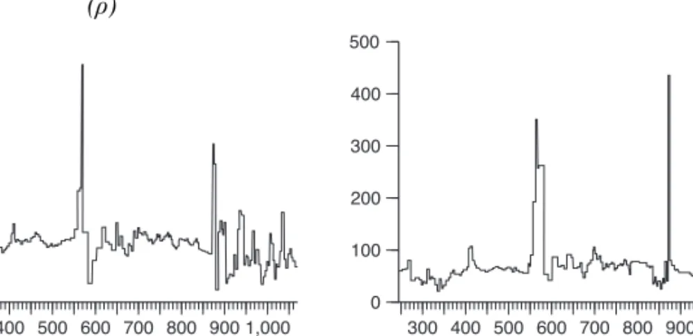
FIGURE 1
Evolution of the series: auction data a. Auction interest rate, nominal
(Rauction)
b. Auction maturity (Mauction)
c. Auction interest rate deflated by seasonally adjusted rate of WPI inflation
(rauction
π )
d. Auction interest rate deflated by depreciation rate of official currency
basket (rauction
ρ )
e. Auction interest rate deflated by interbank interest rate
( i auction
r )
f. Seasonally adjusted rate of WPI inflation
(π)
FIGURE 1 continued g. Depreciation rate of official currency
basket (ρ)
h. Interbank interest rate (i)
Notes: In all panels, the horizontal axis shows the observation numbers. Maturity is measured in 360-day
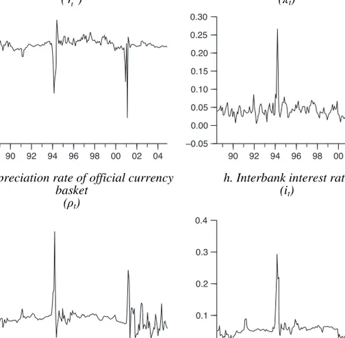
years and other variables are displayed in decimals. FIGURE 2
Evolution of the series: monthly data a. Nominal weighted average auction
interest rate (Rt)
b. Average auction maturity (Mt)
c. Interest rate deflated by seasonally adjusted rate of WPI inflation
(rt π)
d. Interest rate deflated by depreciation rate of official currency basket
(rt ρ)
FIGURE 2 continued e. Interest rate deflated by interbank
interest rate (r ) ti
f. Seasonally adjusted rate of WPI inflation
(πt)
g. Depreciation rate of official currency basket
(ρt)
h. Interbank interest rate (it)
Notes: In all panels, the horizontal axis shows time periods (months). Maturity is measured in 360-day
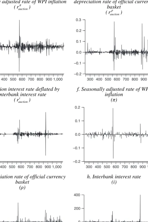
years and other variables are displayed in decimals. FIGURE 3
Evolution of the first differences of the series: auction data a. Auction interest rate, nominal
(Rauction)
b. Auction maturity (Mauction)
FIGURE 3 continued c. Auction interest rate deflated by
seasonally adjusted rate of WPI inflation (rauction
π )
d. Auction interest rate deflated by depreciation rate of official currency
basket (rauction
ρ )
e. Auction interest rate deflated by interbank interest rate
( i auction
r )
f. Seasonally adjusted rate of WPI inflation
(π)
g. Depreciation rate of official currency basket
(ρ)
h. Interbank interest rate (i)
Notes: In all panels, the horizontal axis shows the observation numbers. Maturity is measured in 360-day
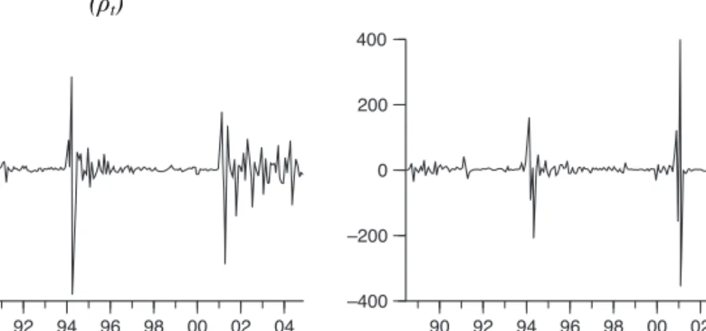
FIGURE 4
Evolution of the first differences of the series: monthly data a. Nominal weighted average auction
interest rate (Rt)
b. Average auction maturity (Mt)
c. Interest rate deflated by seasonally adjusted rate of WPI inflation
(rt π )
d. Interest rate deflated by depreciation rate of official currency basket
(rt ρ)
e. Interest rate deflated by interbank interest rate
(r ) ti
f. Seasonally adjusted rate of WPI inflation
(πt)
FIGURE 4 continued g. Depreciation rate of official currency
basket (ρt)
h. Interbank interest rate (it)
Notes: In all panels, the horizontal axis shows time periods (months). Maturity is measured in 360-day
years and other variables are displayed in decimals.
The levels of the data series and their differences are plotted in Figures 1 and 2 and Figures 3 and 4 respectively. Figures 1 and 2 clearly reflect the trends in the data series and display the effects of the financial crises on our variables. It can be noted that none of the series demonstrates explosive behaviour. Figures 3 and 4 also demonstrate the time-changing variability of the series.
3. Estimation technique and form of estimating equation
A problem of simultaneity is inherent in the data due to the very nature of the treasury auction process, which determines the maturities and interest rates simultaneously. Under these circumstances, the ordinary least squares (OLS) estimates will be biased. The instrumental variable (or two-stage regression) (IV) technique was used to account for this problem in obtaining our parameter estimates.
The first equation form that we investigate is given in equation 1: (1) Real Return=α α0+ 1Maturity+ ε
where Real Return, which is (Nominal Return – X)/(1+X), is obtained as described in subsection III.1 and Maturity is measured in years. X is a deflating variable, such as the rate of inflation, the depreciation rate of the local currency or the interbank interest rate. This form simply helps us to obtain the relationship between real interest rates and maturity.
On the other hand, it is probable that deflating variables, such as rate of inflation, rate of currency depreciation and interbank interest rate, do not affect the real returns in a one-for-one manner, i.e. as in the numerator of the
Real Return expression in equation 1. Therefore we have also employed a
second equation form, in which the deflating variables might have coefficients other than unity. This relaxation is expressed by means of equation 2:
(2) Nominal Return=α α0+ 1Maturity+α2X + ε
where Nominal Return is the nominal interest rate. Equations 1 and 2 are the generic equations that assess the basis for our analysis in the following subsections, where the latter is motivated by Tobin (1965). This suggests that nominal interest rates increase less than the amount by which inflation increases, under the assumption that money and capital are the only forms of wealth and the economy has a decreasing-returns-to-scale production function. Under these circumstances, if the opportunity cost of holding money increases due to higher inflation, then money holdings decrease and capital stock increases. The assumption of decreasing returns to scale causes
the interest rate to increase less than inflation; therefore α2 becomes less
than unity. Regarding how α2 can be less than unity in the case of X being
the interbank interest rate, one might see Cook and Hahn (1989) and Berument and Froyen (2005) for empirical support. Finally, in the case of local currency depreciation, the deflating effect of depreciation can be disproportionate due to the dynamic effects of risk premiums (see Central Bank of the Republic of Turkey (2003)).
When estimating equations 1 and 2 for different subsamples, the reliability of the estimates is a key consideration. Although the IV technique grants that the estimated coefficients are unbiased, the significance of the estimates may be mismeasured if we do not use robust standard errors. In order to avoid such a shortfall, we have employed the Newey–West procedure for non-spherical robust disturbances.
In the next subsection, we present our analysis based on auction data and equation 1. Subsection III.5 presents our results on monthly data under equations 1 and 2.
4. Estimates based on auction data
Estimated coefficients based on the auction data for the return–maturity relationship are reported in Table 3. In the first column, our dependent
variable is rauctionπ , which is regressed on a constant term and bond maturity.
The instrumental variables are the constant term, the first three lags of 1
auction
rπ−
and the lag of Mauction. In the second and third columns, rauctionρ and i
auction
r are
TABLE 3
Real interest-rate–maturity relationships: auction data
Independent variables auction rπ rauctionρ i auction r Whole sample: Jul 1988–Dec 2004 auctions Constant 0.138*** (2.805) 0.159*** (2.203) 0.021*** (3.747) Mauction –0.176*** (–2.354) –0.197* (–1.811) –0.021*** (–2.549) Subsample [1]: Jul 1988–May 2001 auctions Constant 0.096*** (4.375) 0.137*** (3.602) 0.020*** (3.508) Mauction –0.112*** (–3.349) –0.166*** (–2.895) –0.020*** (–2.403) Subsample [2]: Jan 1995–Oct 2000 auctions Constant 0.093*** (7.359) 0.072 (8.337) 0.029 (9.634) Mauction –0.078*** (–4.564) –0.047*** (–4.380) –0.016*** (–3.896) Subsample [3]: Jun 2001–Dec 2004 auctions Constant 0.006 (0.661) 0.002 (0.110) 0.012*** (5.098) Mauction 0.021 (1.622) 0.044 (1.509) –0.009*** (–2.544)
Note: t-statistics are reported in parentheses under the corresponding estimated parameters, where the
underlying standard errors are (White’s) heteroscedasticity-consistent standard errors. *, ** and *** correspond to statistical significance at the 10 per cent, 5 per cent and 1 per cent levels respectively.
deflated with the depreciation rate or the interbank rate, the instrument sets
are modified accordingly. That is, 1
auction
rρ− and i1
auction
r− are used as instruments
when rauctionρ and i auction
r are used as the dependent variables.
Table 3 suggests – for the whole sample – that there is a statistically
significant14 and negative relationship between real interest rates on auctions
and the maturities of newly issued debt, as we hypothesised before. Moreover, the largest coefficient in absolute value is observed when the interest rate is deflated with the depreciation rate. The same observation is valid for subsample [1] – namely, for auctions between July 1988 and May 2001 inclusive. When the focus is shifted to the between-crises episode (subsample [2]), maturity remains statistically significant with a negative sign. Furthermore, it possesses the largest absolute coefficient when the nominal interest rate is deflated by the rate of inflation.
The post-May-2001 subsample displays a different overall picture of the yield curve. When the nominal interest rate is deflated by the inflation rate or rate of currency depreciation, the slope of the estimated yield curve turns
out to be positive, although these estimates of the slope are not statistically significant at the 10 per cent level. This is possibly due to the change in the exchange-rate regime. Although the exchange rate was a useful indicator of expected inflation before the 2001 financial crisis, it is not so after February 2001, when the exchange rate was allowed to float freely.
It is worth noting that the slope of the yield curve remains negative and statistically significant for the post-May-2001 subsample when we compute the real auction return in excess of the interbank interest rate. This possibly reflects the change in people’s perception of the economic dynamics after May 2001.
The above-mentioned change from pre-June-2001 to post-May-2001 episode is worth further elaboration. In the absence of a confidence crisis, an upward-sloping yield curve is associated with expectations of ‘increasing inflation’, i.e. investors require higher nominal returns if they believe that the future course of inflation will trend upwards. However, the presence of a confidence crisis (for example, low confidence) reverses this picture, as elaborated in Section II. That is, there is no period before 2001 during which inflation continuously falls, and this should normally imply an upward-sloping yield curve. However, the risk profile of the Turkish-lira-denominated domestic debt causes the slope to be downwards, rather than upwards, in the pre-June-2001 episode.
In the post-May-2001 episode, both actual consumer price inflation and inflation expectations have been steadily falling. This is clearly a textbook case of a downward-sloping yield curve. Our empirical estimates, however, reveal the opposite, probably indicating the continuation of the high risk profile of the Treasury.
5. Estimates based on monthly data
Our auction-based estimates depict a negative linkage between the interest rate of government auctions and auction maturity, confirming our theoretical finding in Section II for the pre-June-2001 period. This subsection provides evidence from the monthly data. Due to the lack of treasury auctions in December 1999 and December 2000, there are two missing values in the maturity series. The State Planning Organisation provided observations for those months by substituting information on the Treasury’s sale of bonds to public institutions. This anomaly of data is handled by defining intercept dummy variables for each of the two months. These dummy variables are included in both the functional specification and the set of instrumental variables, so as to control for the effect of missing observations.
TABLE 4
Real interest-rate–maturity relationships: monthly data
Independent variables t rπ rtρ i t r Whole sample: Jul 1988–Dec 2004 Constant 0.069*** (3.220) 0.087* (1.773) 0.028*** (2.271) Mt –0.063*** (–2.242) –0.082 (–1.265) –0.0289* (–1.737) D9912 0.031 (0.949) 0.067 (0.873) 0.014 (0.757) D0012 0.012* (1.905) 0.022 (1.637) –0.109*** (–27.964) Subsample [1]: Jul 1988–May 2001
Constant 0.071*** (3.668) 0.092* (1.830) 0.010 (0.543) Mt –0.065*** (–2.475) –0.091 (–1.367) –0.002 (–0.102) D9912 0.031 (1.009) 0.077 (0.999) –0.017 (–0.653) D0012 0.011* (1.663) 0.026* (1.834) –0.115*** (–25.646) Subsample [2]: Jan 1995–Oct 2000
Constant 0.088*** (5.818) 0.067*** (5.729) 0.027*** (7.621) Mt –0.061*** (–3.822) –0.035*** (–2.805) –0.010*** (–2.368) D9912 0.008 (0.505) –0.004 (–0.339) –0.019*** (–3.837) Subsample [3]: Jun 2001–Dec 2004
Constant 0.016*** (2.273) –0.007 (–0.263) 0.014*** (6.041) Mt 0.004 (0.352) 0.055 (1.601) –0.011*** (–3.976)
Notes: t-statistics are reported in parentheses under the corresponding estimated parameters, where the
underlying standard errors are (White’s) heteroscedasticity-consistent standard errors. *, ** and *** correspond to statistical significance at the 10 per cent, 5 per cent and 1 per cent levels respectively.
D0012 is not usable in subsample [2], and neither D9912 nor D0012 is usable in subsample [3], to avoid
singularity.
In our first series of regressions, we use rtπ, rtρ and rti as the
left-hand-side variables. The regressors are the constant term, maturity Mt and the
dummy variables for December 1999 (D9912) and December 2000 (D0012). We use the constant term, the two dummy variables and one to four lags of
it, πt and ρt as our instrumental variables. The estimates in Table 4 suggest –
for the whole sample – a negative relationship between real bond return and maturity, supporting our previous findings in the auction-based regressions.
When the nominal interest rate is deflated with the inflation rate, the slope estimate of the yield curve is significant at 1 per cent; when it is deflated by the interbank interest rate, the significance is at the 10 per cent level.
Although the yield curve has a negative slope for rtρ, this estimate is
insignificant. Table 4 further replicates these estimations for our three subsamples. In subsample [1], we observe a significantly negative slope estimate in the first column only. The real interest rate computed using the depreciation rate or the interbank interest rate does not have a statistically significant association with maturity in subsample [1].
Estimates for subsample [2] suggest a negatively sloped yield curve, regardless of the deflating variable. All these estimates are statistically significant at the 1 per cent level. The insignificance disappears when the crises are excluded from subsample [1]. This is mainly due to the fact that during the crisis episodes, the series under consideration display erratic behaviour and act as outliers.
The last panel of Table 4 closely mimics that of Table 3, i.e. the estimated yield curves attain positive but insignificant slopes when inflation or depreciation rates are used as deflators in subsample [3], while the case of the interbank interest rate still suggests a negatively sloped yield curve after May 2001.
One may be sceptical of the regressions presented in Table 4 since a coefficient of unity is imposed on the deflating variable in each of the regressions. Following Tobin (1965), Cook and Hahn (1989) and inflation-risk-premium arguments that a change in the deflating variables may not be
reflected in the nominal interest rate on a one-for-one basis,15 we estimate
another set of regressions in which the monthly nominal interest rate, Rt, is
regressed on the constant term, Mt, D9912, D0012 and either πt, ρt or it, and
where the set of instrumental variables consists of the constant term, the two
dummy variables and one to three lags of πt, ρt and it. Our IV estimates of
these specifications are reported in Table 5, which suggests the previously observed negative relationship between interest rates and maturity variables
with tighter levels of significance.16 However, there are some changes in the
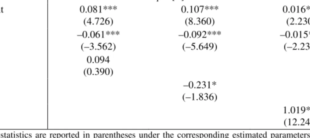
pattern of slope estimates across subsamples and across deflating variables. For instance, the whole sample suggests significantly negative estimates in all three specifications. In contrast to what we have observed in Table 4, in Table 5 these significant and negative estimates are maintained in subsample [1]. Moreover, subsamples [2] and [3] also suggest negatively sloped yield curves for all specifications except for the third in subsample [2]. In sum, the overall picture suggests a negatively sloping yield curve.
15See Berument and Malatyali (2001) for elaboration on this for Turkey.
16The same estimation could not be performed for the specifications in the previous subsection due to
TABLE 5
Nominal interest-rate–maturity relationships: monthly data
Independent variables
Rt Rt Rt
Whole sample: Jul 1988–Dec 2004 Constant 0.124*** (5.017) 0.162*** (7.947) 0.111*** (5.272) Mt –0.111*** (–3.947) –0.146*** (–5.758) –0.098*** (–3.702) D9912 0.101*** (2.763) 0.155*** (5.133) 0.098*** (3.150) D0012 0.013*** (2.275) 0.016*** (2.631) –0.042*** (–3.062) πt 0.488*** (3.111) ρt 0.161* (1.909) it 0.387*** (4.153) Subsample [1]: Jul 1988–May 2001
Constant 0.103*** (5.123) 0.131*** (7.121) 0.089*** (4.379) Mt –0.075*** (–3.337) –0.094*** (–4.029) –0.056*** (–2.208) D9912 0.055* (1.939) 0.088*** (3.198) 0.045 (1.532) D0012 –0.001 (–0.129) –0.003 (–0.476) –0.050*** (–5.482) πt 0.446*** (3.044) ρt 0.125*** (2.057) it 0.331*** (5.193) Subsample [2]: Jan 1995–Oct 2000
Constant 0.105*** (3.378) 0.089*** (3.452) 0.008 (0.239) Mt –0.069*** (–3.288) –0.051*** (–2.712) –0.015 (–0.827) D9912 0.019 (0.639) 0.012 (0.553) –0.017 (–0.868) πt 0.780* (1.929) ρt 0.831*** (2.672) it 1.436*** (4.297)
TABLE 5 continued
Independent variables
Rt Rt Rt
Subsample [3]: Jun 2001–Dec 2004 Constant 0.081*** (4.726) 0.107*** (8.360) 0.016*** (2.230) Mt –0.061*** (–3.562) –0.092*** (–5.649) –0.015*** (–2.233) πt 0.094 (0.390) ρt –0.231* (–1.836) it 1.019*** (12.248)
Notes: t-statistics are reported in parentheses under the corresponding estimated parameters, where the
underlying standard errors are (White’s) heteroscedasticity-consistent standard errors. *, ** and *** correspond to statistical significance at the 10 per cent, 5 per cent and 1 per cent levels respectively.
D0012 is not usable in subsample [2], and neither D9912 nor D0012 is usable in subsample [3], to avoid
singularity.
Due to the persistence of the variables of concern, there might be a problem of serial correlation in our estimates. Lagged values of the dependent variable have not been included in either Table 4 or Table 5. This kind of specification may raise suspicion about the robustness of the results. For instance, if real interest rates and maturity are both serially correlated variables, estimating an equation without a lagged dependent variable, or without correction for serial correlation, may make the maturity variable statistically significant only because it is a proxy for the lagged dependent
variable or the serial correlation correction.17 Consequently, we have
re-generated our specifications in Tables 4 and 5 by adding three lagged values of dependent and, in the case of the nominal-interest-rate regressions,
deflating variables as regressors.18 Tables 6 and 7 are the counterparts of
Tables 4 and 5 respectively.19
17See Hamilton (1994, pages 557–62) for a discussion of these issues.
18The choice of three lags is due to the frequency of the financial statements prepared for the majority
of financial institutions in Turkey. The basic results were robust for a set of alternative lag structures.
19We have also performed the Ljung–Box (1978) tests (up to six lags) and could reject the null
hypothesis of no autocorrelation for all specifications reported in Tables 4 and 5 (not reported in the paper).
TABLE 6
Real interest-rate–maturity relationships: monthly data
Whole sample: Jul 1988–Dec 2004 Subsample [1]: Jul 1988–May 2001 Subsample [2]: Jan 1995–Oct 2000 Subsample [3]: Jun 2001–Dec 2004
t rπ rt ρ i t r rt π t rρ i t r rt π t rρ i t r rt π t rρ i t r Constant 0.046* (1.795) 0.067 (1.282) 0.061 (1.244) 0.050*** (2.565) 0.077 (1.506) 0.017 (0.521) 0.036*** (3.011) 0.025*** (2.238) 0.015 (1.366) 0.006 (1.207) –0.004 (–0.153) 0.010*** (2.313) Mt –0.050 (–1.438) –0.068 (–0.996) –0.080 (–1.136) –0.055*** (–2.070) –0.081 (–1.245) –0.018 (–0.350) –0.026*** (–2.402) –0.014 (–1.498) –0.012 (–1.060) 0.002 (0.335) 0.036 (0.956) –0.010*** (–2.245) D9912 0.019 (0.483) 0.054 (0.684) 0.074 (0.910) 0.024 (0.797) 0.070 (0.957) 0.001 (0.020) –0.018* (–1.887) –0.019*** (–2.062) –0.009 (–0.797) D0012 0.016*** (2.132) 0.020 (1.413) –0.084*** (–4.741) 0.017*** (2.644) 0.023* (1.762) –0.101*** (–5.760) 1 t rπ− 0.491*** (3.258) 0.475*** (3.181) 0.448*** (2.314) 0.696*** (5.148) 2 t rπ− 0.026 (0.168) 0.018 (0.119) 0.134 (0.714) 0.023 (0.188) 3 t rπ− 0.063 (0.526) 0.085 (0.806) 0.015 (0.099) –0.122 (–1.282) 1 t rρ− 0.441*** (2.822) 0.531*** (2.556) 0.221 (1.337) 0.318* (1.932) 2 t rρ− –0.117 (–0.778) –0.284 (–1.641) 0.254** (1.985) 0.002 (0.017) 3 t rρ− 0.050 (0.479) 0.097 (0.793) 0.165 (1.364) –0.016 (–0.155) 1 i t r− 0.214 (1.321) 0.227 (1.297) 0.469*** (3.388) 0.627*** (4.529) 2 i t r− 0.432 (1.282) 0.340 (1.166) 0.059 (0.333) –0.206 (–1.579) 3 i t r− 0.083 (0.413) –0.045 (–0.212) 0.194* (1.654) 0.077 (0.666)
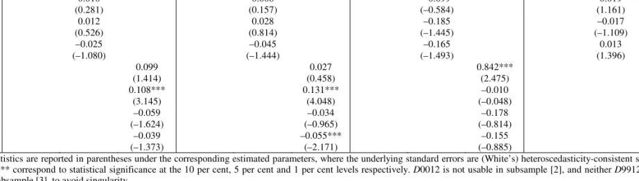
TABLE 7
Nominal interest-rate–maturity relationships: monthly data
Whole sample: Jul 1988–Dec 2004 Subsample [1]: Jul 1988–May 2001 Subsample [2]: Jan 1995–Oct 2000 Subsample [3]: Jun 2001–Dec 2004
Rt Rt Rt Rt Rt Rt Rt Rt Rt Rt Rt Rt Constant 0.005** (1.962) 0.007*** (2.744) 0.005 (1.593) 0.010*** (2.608) 0.009*** (2.981) 0.007*** (2.331) 0.006 (0.725) 0.015*** (2.641) –0.001 (–0.101) –0.017*** (–2.086) –0.006 (–0.949) 0.010 (1.604) Mt –0.005* (–1.806) –0.006** (–1.964) –0.005** (–2.018) –0.007*** (–2.243) –0.007*** (–2.133) –0.006** (–2.015) –0.010* (–1.779) –0.007** (–1.852) –0.003 (–0.738) 0.016*** (2.215) –0.006 (–1.023) –0.009 (–1.629) D9912 –0.014*** (–2.980) –0.011*** (–2.868) –0.010*** (–3.097) –0.011*** (–2.417) –0.010*** (–2.543) –0.010*** (–2.774) –0.055*** (–3.689) –0.021*** (–3.330) –0.019*** (–3.714) D0012 0.008*** (9.083) 0.008*** (8.939) –0.008 (–0.945) 0.007*** (4.427) 0.008*** (4.448) –0.001 (–0.105) Rt–1 0.857*** (7.470) 0.799*** (6.704) 0.786*** (7.022) 0.845*** (6.969) 0.766*** (5.343) 0.748*** (6.557) 0.695*** (2.702) 0.543*** (3.285) 0.576*** (3.889) 0.869*** (5.869) 0.866*** (5.854) 0.698*** (3.855) Rt–2 –0.163 (–1.034) –0.086 (–0.587) –0.034 (–0.218) –0.147 (–0.819) –0.076 (–0.465) 0.016 (0.099) –0.065 (–0.182) 0.046 (0.234) 0.086 (0.538) 0.121 (0.537) 0.094 (0.361) –0.278 (–1.152) Rt–3 0.190 (1.641) 0.186* (1.710) 0.137 (1.419) 0.187 (1.426) 0.192 (1.497) 0.126 (1.132) –0.037 (–0.148) 0.179 (1.276) 0.010 (0.083) 0.010 (0.081) 0.045 (0.288) 0.159 (0.782) πt 0.162 (1.622) 0.109 (1.249) 1.697*** (2.802) 0.439*** (3.011) πt–1 0.002 (0.031) 0.019 (0.237) –0.758*** (–2.190) –0.149* (–1.733) πt–2 –0.019 (–0.360) –0.015 (–0.287) –0.307* (–1.659) –0.091 (–1.383) πt–3 –0.022 (–0.348) –0.042 (–0.572) 0.208 (1.294) 0.048 (1.220)
TABLE 7 continued
Whole sample: Jul 1988–Dec 2004 Subsample [1]: Jul 1988–May 2001 Subsample [2]: Jan 1995–Oct 2000 Subsample [3]: Jun 2001–Dec 2004
Rt Rt Rt Rt Rt Rt Rt Rt Rt Rt Rt Rt ρt 0.081* (1.891) 0.084 (1.622) 0.664*** (2.266) 0.042* (1.690) ρt–1 0.010 (0.281) 0.008 (0.157) –0.099 (–0.584) 0.019 (1.161) ρt–2 0.012 (0.526) 0.028 (0.814) –0.185 (–1.445) –0.017 (–1.109) ρt–3 –0.025 (–1.080) –0.045 (–1.444) –0.165 (–1.493) 0.013 (1.396) it 0.099 (1.414) 0.027 (0.458) 0.842*** (2.475) 0.751 (1.463) it–1 0.108*** (3.145) 0.131*** (4.048) –0.010 (–0.048) –0.264 (–0.314) it–2 –0.059 (–1.624) –0.034 (–0.965) –0.178 (–0.814) 0.107 (0.225) it–3 –0.039 (–1.373) –0.055*** (–2.171) –0.155 (–0.885) –0.193 (–0.450)
Notes: t-statistics are reported in parentheses under the corresponding estimated parameters, where the underlying standard errors are (White’s) heteroscedasticity-consistent standard errors.
*, ** and *** correspond to statistical significance at the 10 per cent, 5 per cent and 1 per cent levels respectively. D0012 is not usable in subsample [2], and neither D9912 nor D0012 is usable in subsample [3], to avoid singularity.
Notes to Table 6: t-statistics are reported in parentheses under the corresponding estimated parameters,
where the underlying standard errors are (White’s) heteroscedasticity-consistent standard errors. *, ** and *** correspond to statistical significance at the 10 per cent, 5 per cent and 1 per cent levels respectively. D0012 is not usable in subsample [2], and neither D9912 nor D0012 is usable in subsample [3], to avoid singularity.
The estimates of Table 6 suggest the same negative relationship between maturity and real interest rates. However, the level of statistical significance has dropped considerably. For the whole sample, maturity has negative coefficients in all cases, but they are not statistically significant. In subsample [1], the coefficient of maturity is negative and significant only for rtπ. For rtρ and rti, it is negative as well, but not statistically significant. Subsample [2] suggests a similar pattern of estimates, although the slope of
the yield curve is smaller in magnitude. In the last subsample, for rtπ and
t
rρ, the coefficient of maturity turns positive, but these positive estimates
are not statistically significant; for i
t
r , the maturity variable has a negative
and significant coefficient estimate, implying a negatively sloped yield curve.
Similar to the relationship between Table 6 and Table 4, Table 7 verifies the findings of Table 5. Indeed, inclusion of the lagged dependent variable as a regressor remedied the residuals’ autocorrelation problem in practically
all the specifications and subsamples, without altering the key findings.20
Although the aforementioned non-normality of data in the whole sample and in subsample [1] affected the normality of the residuals in the estimations
for these sample episodes, it did not change the quality of our findings.21
As mentioned previously, we have also assessed the robustness of our specifications to the existence of the financial crises in our sample span. The Chow test statistics, which are presented in Table 8, provide support for our segmentation of the whole sample into subsamples.
All in all, the negative linkage between interest rates and maturity that we have revealed using auction data, presented in Table 3, remained intact despite changes in the data structure – i.e. using monthly data instead of auction data – and despite different specifications – i.e. specifications that include, versus those that do not include, the lagged values of the dependent variable as right-hand-side variables. However, the signs and significance levels of our parameter estimates do differ in the pre-June-2001 and post-May-2001 samples.
The findings for the pre-June-2001 subsamples are in line with our elaboration and interpretation of Alesina, Prati and Tabellini (1990), the model that is presented in Section II, as well as Giavazzi and Pagano (1990),
20Based on the Ljung–Box (1978) tests (not reported). 21Based on Jarque–Bera (1987) tests (not reported).
Alesina et al. (1992), Calvo and Guidotti (1992) and Missale and Blanchard (1994).
TABLE 8 Chow breakpoint tests
Breakpoints tested Deflating variable
πt ρt it Table 3 specification 1994:04 and 2001:02 in the whole sample 22.88*** (0.000) 20.59*** (0.000) 11.90*** (0.000) 1994:04 in the pre-November-2000 subsample 42.18*** (0.000) 40.91*** (0.000) 25.50*** (0.000) 2001:02 in the post-December-1994 subsample 3.85** (0.022) 2.22 (0.109) 14.46*** (0.000) Table 4 specification 1994:04 and 2001:02 in the whole sample 5.66*** (0.000) 8.39*** (0.000) 3.52*** (0.008) 1994:04 in the pre-November-2000 subsample –0.56 (1.000) –5.90 (1.000) 11.76*** (0.000) 2001:02 in the post-December-1994 subsample 11.85*** (0.000) 6.34*** (0.002) 5.89*** (0.004) Table 5 specification 1994:04 and 2001:02 in the whole sample 4.90*** (0.000) 6.20*** (0.000) 9.04*** (0.000) 1994:04 in the pre-November-2000 subsample 4.46*** (0.005) 5.62*** (0.001) 10.31*** (0.000) 2001:02 in the post-December-1994 subsample 9.99*** (0.000) 28.68*** (0.000) 17.08*** (0.000) Table 6 specification 1994:04 and 2001:02 in the whole sample 1.86* (0.053) 2.24** (0.017) 4.55*** (0.000) 1994:04 in the pre-November-2000 subsample –0.87 (1.000) –2.93 (1.000) 7.61*** (0.000) 2001:02 in the post-December-1994 subsample 2.94** (0.015) 2.85** (0.018) 1.84 (0.109) Table 7 specification 1994:04 and 2001:02 in the whole sample 3.15*** (0.000) 2.94*** (0.000) 1.35 (0.159) 1994:04 in the pre-November-2000 subsample 2.25** (0.022) 1.09 (0.367) 1.23 (0.276) 2001:02 in the post-December-1994 subsample 1.44 (0.180) 1.22 (0.288) 1.27 (0.260)
Notes: F-statistics and the p-values (in parentheses) of the Chow tests are provided in the table. *, ** and
*** correspond to rejection of the null hypothesis at the significance levels of 10 per cent, 5 per cent and 1 per cent respectively. For each specification, three tests are computed. In the first test, the null hypothesis that no structural break exists is jointly tested for April 1994 and February 2001 over the whole-sample estimates. In the second test, the April 1994 structural break is tested over the pre-November-2000 subsample. The third test considers the February 2001 break over the post-December-1994 period.
IV. Discussion and concluding remarks
1. DiscussionIn subsection III.4, the auction-based estimates suggested that the slope of the yield curve is negative for Turkish treasury auctions, which is repeatedly revealed in the whole sample, in the July 1988 to May 2001 sample and in the January 1995 to October 2000 sample. However, we observe a change in this pattern from June 2001, when the maturity variable attains a significantly negative coefficient estimate only when the nominal interest rate on auctions is deflated by the interbank interest rate to obtain the real interest rate. Maturity does not have a significant coefficient in the other regressions. At this point, it is important to summarise to what extent our empirical findings remain intact and where they display a pattern change.
First of all, the findings on auction data are further supported by our monthly estimates in subsection III.5, regardless of the relationship estimated for nominal or real measures of return. That is, whether we estimate equation 1 or equation 2 of subsection III.3, we have revealed the same evidence as we had on auction data.
Second, the between-crises subsample is the most stable episode in terms of the durability of empirical findings. This situation augments our views on the low public confidence in the governments’ debt management policies in Turkey for the 1995–2000 period.
Third, the post-May-2001 sample yields a radical pattern change. In most cases, in the post-May-2001 episode, we observe that the real auction return computed by using the interbank interest rate is still negatively associated with maturity of debt. However, the sign of the coefficient on maturity turns positive in other cases, along with lower statistical significance. That is, people’s perception with regard to the rate of inflation and the depreciation of the Turkish lira must have changed after May 2001. In the light of recent Turkish policymaking experience, this might be intuitive. Indeed, the policy view of the Central Bank of the Republic of Turkey toward reducing inflation was formulated and has been implemented in terms of the ‘implicit inflation targeting’ framework and the Bank was set to an ‘independent’ position starting in April–May 2001. After this date, the Bank manifested its fundamental goal as the stability of prices. The exchange-rate regime, in the
same episode, was set as the ‘floating exchange rate’ regime.22 Eventually,
the changes in the public perception of inflation and currency depreciation can be considered as a consequence of these changes in the monetary
policymaking framework.23
22The exchange-rate regime is determined by the government, together with the Central Bank of the
Republic of Turkey, and implemented by the Central Bank, as required by the Central Bank Law.
23It should also be noted that the primary surplus target of the stabilisation programme started in June
2. Concluding remarks
On the theoretical front, the further elaboration of the Alesina, Prati and Tabellini (1990) model, as presented in Section II and Appendix A, suggests a negative relationship between the treasury auction interest rates and auction maturity, under the assumption of a non-zero default risk and confidence crises. Our study provides empirical evidence from the Turkish economy on this relationship. We have performed our analysis through two types of data-sets. First, we have used a data-set that contains the data from each treasury auction. Second, we have used monthly data, which were obtained from the first data-set through aggregation.
The finding of a downward-sloping yield curve is quite consistent with some specific conditions of the Turkish economy, such as chronic high and volatile levels of inflation, a high and volatile default risk, frequent occurrences of financial crisis, an inflation–devaluation cycle and the low credibility of policymakers, specifically until mid-2001. Due to real return and default risks, those conditions shape the maturity–return relationship in a different way from the case for developed countries. In this set-up, the low credibility of policymakers makes shorter auction maturities and higher interest rates necessary. Consequently, once the market is unable to generate its long-term assets, returns on treasury bills are pushed far above the generally prescribed levels. As far as the outcome is concerned, it can be argued that such management of debt is expected to be self-promoting and further unsustainability of debt is unavoidable. The post-May-2001 developments should be studied in more depth in order to reach a better understanding of possible changes in macroeconomic fundamentals. This may gain feasibility over time, as more observations are accumulated.
Appendix: The Alesina, Prati and Tabellini (1990) model
Here, we present a formal model that reveals a negative relationship between the treasury auction maturity and interest rates. In order to do this, we employ an infinite-horizon model, based on that of Alesina, Prati and Tabellini (1990), which maximises a representative individual’s lifetime utility function and minimises the government’s loss function.
In this model, a small economy is inhabited by an infinitely-lived individual who maximises her lifetime utility:
generate new debt. As the expenditures of the political authority are radically restricted, the scepticism regarding the rollover of existing debt stock was limited after May 2001. Another important ingredient of the recent political climate of Turkey can be marked as the switch from a sequence of coalitional governments to a majority cabinet in the Grand National Assembly. These observations highlight the reduction of fiscal risks and political uncertainties.