a dissertation submitted to
the department of industrial engineering
and the institute of engineering and science
of bilkent university
in partial fulfillment of the requirements
for the degree of
doctor of philosophy
By
H¨unkˆar Toyo˘glu
January, 2010
Assoc. Prof. Bahar Yeti¸s Kara (Supervisor)
I certify that I have read this thesis and that in my opinion it is fully adequate, in scope and in quality, as a dissertation for the degree of doctor of philosophy.
Assoc. Prof. Oya Ekin Kara¸san
I certify that I have read this thesis and that in my opinion it is fully adequate, in scope and in quality, as a dissertation for the degree of doctor of philosophy.
Prof. Barbaros C¸ . Tansel ii
Prof. Erdal Erel
I certify that I have read this thesis and that in my opinion it is fully adequate, in scope and in quality, as a dissertation for the degree of doctor of philosophy.
Assoc. Prof. Osman O˘guz
Approved for the Institute of Engineering and Science:
Prof. Mehmet B. Baray Director of the Institute
DESIGN ON THE BATTLEFIELD
H¨unkˆar Toyo˘glu
PhD. in Industrial Engineering
Supervisors: Assoc. Prof. Bahar Yeti¸s Kara and Assoc. Prof. Oya Ekin Kara¸san
January, 2010
Ammunition has been the most prominent factor in determining the outcome of combat. In this dissertation we study a military logistics problem in which ammunition requirements of the combat units, which are located on the battle-field, are to be satisfied in the right amount when and where they are needed. Our main objective is to provide a decision support tool that can help plan ammunition distribution on the battlefield. We demonstrate through an exten-sive literature review that the existing models are not capable of handling the specifics of our problem. Hence, we propose a mathematical programming model considering arc-based product-flow with O(n4) decision variables and constraints.
The model is a three-layer commodity-flow location routing formulation that dis-tributes multiple products, respects hard time windows, allows demand points to be supplied by more than one vehicle or depot, and locates facilities at two differ-ent layers. We then develop a new mathematical programming model with only
O(n3) decision variables and constraints by considering node-based product-flow.
We derive several valid inequalities to speed up the solution time of our models, illustrate the performance of the models in several realistically sized scenarios, and report encouraging results. Based on these mathematical models we propose two three-phase heuristic methods: a routing-first second and a location-first routing-second heuristic. The computational results show that complex real world problems can effectively be solved in reasonable times with the proposed heuristics. Finally, we introduce a dynamic model that designs the distribution system in consecutive time periods for the entire combat duration, and show how the static model can be utilized in dynamic environments.
Keywords: Location routing, logistics, distribution, network design.
MUHAREBE SAHASINDA MOBIL BIR M ¨
UHIMMAT
DA ˘
GITIM SISTEMI TASARIMI
H¨unkˆar Toyo˘glu
End¨ustri M¨uhendisli˘gi, Doktora
Tez Y¨oneticileri: Do¸c. Dr. Bahar Yeti¸s Kara ve Do¸c. Dr. Oya Ekin Kara¸san
Ocak, 2010
M¨uhimmat sava¸sın sonucunu belirleyen en ¨onemli etmendir. Bu doktora ¸calı¸smasında muharebe sahasında bulunan birliklerin m¨uhimmat ihtiya¸clarının istenen yer ve zamanda ve do˘gru miktarda kar¸sılanması gereken askeri bir lojistik problem incelenmi¸stir. Esas amacımız muharebe sahasında m¨uhimmat da˘gıtımının planlanmasına yardımcı olabilecek bir karar destek sistemi geli¸stirmektir. Kapsamlı bir yazılı eser taramasından sonra ¨onceden geli¸stirilmi¸s olan modellerin problemimizi ¸c¨ozmeye yeterli olmadıkları g¨osterilmi¸stir. Bu sebe-ple ayrıt tabanlı ¨ur¨un akı¸sına dayanan, O(n4) sayıda karar de˘gi¸skeni ve kısıt i¸ceren
bir matematiksel model ¨onerilmi¸stir. S¨oz konusu model ¨u¸c katmanlı ¨ur¨un akı¸s modeli olup birden fazla ¨ur¨un da˘gıtmakta, esnek olmayan zaman pencerelerini i¸cermekte, ihtiya¸c noktalarının birden fazla ara¸c veya depo tarafından desteklen-mesine izin vermekte ve iki farklı katmana tesis yerle¸stirmektedir. Daha sonra d¨u˘g¨um tabanlı ¨ur¨un akı¸sına dayanan ve sadece O(n3) sayıda karar de˘gi¸skeni
ve kısıt i¸ceren bir matematiksel model geli¸stirilmi¸stir. Modellerin ¸c¨oz¨um za-manının iyile¸stirilmesi maksadıyla bir¸cok ge¸cerli e¸sitsizlik geli¸stirilmi¸s, bazı ger¸cek boyutlu senaryolar ¨uzerinde modellerin performansları denenmi¸s ve iyi sonu¸clar elde edildi˘gi g¨osterilmi¸stir. Bu modeller temel alınarak yol atama-yerle¸stirme ve yerle¸stirme-yol atama olmak ¨uzere ¨u¸c a¸samalı iki ayrı bulgusal y¨ontem geli¸stirilmi¸stir. Hesaplama sonu¸cları ¨onerilen y¨ontemler sayesinde karma¸sık ger¸cek problemlerin makul zamanlar i¸cerisinde ¸c¨oz¨ulebildi˘gini g¨ostermektedir. Son olarak, muharebe boyunca birbirini izleyen zaman aralıklarında da˘gıtım a˘gını tasarlayan dinamik bir model geli¸stirilmi¸s ve statik modelden dinamik ortamlarda nasıl faydalanılabilece˘gi g¨osterilmi¸stir.
Anahtar s¨ozc¨ukler : A˘g tasarımı, yer se¸cimi ve yol atama, lojistik, da˘gıtım.
Sabır ve ¨ozveriyle her zaman yanımda olan
sevgi dolu
e¸sim Arzu’ya
Varlıkları ile hayatımıza anlam veren
mutluluk kayna˘gı
I would like to thank the faculty members and administrative staff of the De-partment of Industrial Engineering. I appreciate their collective assistance to complete this dissertation. I also extend my thanks to them for the emotional support they provided, and for helping me get through the difficult times. In par-ticular, I am especially grateful to Assoc. Prof. Hande Yaman and Prof. ¨Ulk¨u G¨urler for providing me perpetual encouragement and support.
I would like to express my appreciation to my doctoral committee members. I am deeply indebted to Prof. Barbaros C¸ . Tansel for his advice and encouragement throughout my doctoral studies, and for guiding me to a high research standard. He is one of the best teachers that I have had and I am fortunate to have the opportunity to work with him. I would like to thank Prof. Erdal Erel for his insightful comments and constructive criticisms during my research, and to Assoc. Prof. Osman O˘guz and Assoc. Prof. Canan Sepil for accepting to read and review this dissertation.
I would like to offer my deepest and sincerest gratitude to my supervisors Assoc. Prof. Bahar Yeti¸s Kara and Assoc. Prof. Oya Ekin Kara¸san, who have been always there to listen and give advice. Without their continuous friendship, support and motivation this dissertation would not have been completed. I could not wish for better supervisors.
Finally, and most importantly, I wholeheartedly thank my family. My un-derstanding, patient and unselfishly loving wife, Arzu Toyo˘glu, is my constant source of support and strength throughout this endeavor. Our son and daughter, Atakan and Duru Toyo˘glu, are the joy of our lives, and they always remind me about what is important in life. I am indebted to them more than they know and this dissertation is impossible without them.
1 Introduction and Motivation 2
2 Problem Definition and Related Literature 5
2.1 Problem definition . . . 5
2.2 Literature review . . . 7
2.3 Comparison . . . 14
3 Static 4-Index Model Development 20 3.1 Constraints . . . 23
3.1.1 Product flow balance constraints . . . 23
3.1.2 Vehicle flow balance constraints . . . 24
3.1.3 Capacity constraints . . . 25
3.1.4 Relation constraints . . . 26
3.1.5 Time related constraints . . . 27
3.2 Objective function . . . 29
3.3 Model . . . 30 viii
3.4 Valid inequalities . . . 30
3.4.1 Valid inequalities related to product flow balance . . . 31
3.4.2 Valid inequalities related to vehicle flow balance . . . 31
3.4.3 Valid inequalities related to variable and logical relations . 32 3.4.4 Valid inequalities related to time . . . 34
4 Static 3-Index Model Development 35 4.1 Constraints . . . 36
4.1.1 Product flow balance constraints . . . 36
4.1.2 Vehicle flow balance constraints . . . 37
4.1.3 Capacity constraints . . . 37
4.1.4 Relation constraints . . . 38
4.1.5 Time related constraints . . . 40
4.2 Model . . . 41
4.3 Valid inequalities . . . 41
4.4 Model comparison . . . 44
5 Computational Experiments (Part I) 47 5.1 Experiments on test bed problem instances . . . 47
5.2 4-index model . . . 48
5.3 3-index model . . . 55
6 Computational Experiments (Part II) 64
6.1 Small size instances . . . 65
6.2 Large size instances . . . 70
6.3 4-index model . . . 75
6.4 3-index model . . . 80
6.5 Findings with valid inequalities . . . 83
6.5.1 4-index model . . . 84
6.5.2 3-index model . . . 87
6.6 Findings without valid inequalities . . . 87
7 Heuristic Solution Methodology 95 7.1 VRP first-LRP second heuristic . . . 96
7.1.1 Phase 1. Clustering . . . 98
7.1.2 Phase 2. Vehicle routing problem (VRP) . . . 99
7.1.3 Phase 3. Location routing problem (LRP) . . . 106
7.2 LRP first-VRP second heuristic . . . 109
7.2.1 Phase 1. Clustering . . . 109
7.2.2 Phase 2. Location routing problem (LRP) . . . 109
7.2.3 Phase 3. Vehicle routing problem (VRP) . . . 112
8 Computational Experiments (Part III) 115 8.1 4-index model . . . 115
8.1.1 VRP first-LRP second heuristic . . . 115
8.1.2 LRP first-VRP second heuristic . . . 119
8.2 3-index model . . . 122
8.2.1 VRP first-LRP second heuristic . . . 122
8.2.2 LRP first-VRP second heuristic . . . 122
8.3 Findings . . . 125
8.3.1 4-index model . . . 125
8.3.2 3-index model . . . 126
8.3.3 Comparison of the heuristics . . . 128
8.3.4 Comparison of the models . . . 129
9 Dynamic Model Development 130 9.1 Model development . . . 130
9.2 Sample scenario . . . 136
10 Static Model in Real Life 139 10.1 Multi-period Planning with the Static Model . . . 139
10.2 Facing Unplanned Contingencies with the Static Model . . . 141
11 Summary and Conclusion 144
2.1 Mobile ammo distribution system on the battlefield . . . 6
3.1 Routes of commercial and special ammo trucks . . . 21
4.1 Node-based product flow decision variables . . . 36
6.1 Organization of a representative land force . . . 66
6.2 The corps’ layout plan on the battlefield . . . 67
6.3 Ammunition groups . . . 67
6.4 The corps’ layout plan on the battlefield . . . 71
6.5 Layout of the base scenario solution . . . 74
6.6 Detailed solution of the first brigade . . . 74
6.7 4-index model run times with the first objective . . . 90
6.8 4-index model run times with the second objective . . . 91
6.9 3-index model run times with the second objective . . . 92
6.10 Comparison of the general statistics of 4-index and 3-index models 93 6.11 Comparison summary of the 4-index and 3-index models . . . 94
7.1 Flowchart for the VRP first-LRP second heuristic method . . . . 97 7.2 Flowchart for the LRP first-VRP second heuristic method . . . . 110 9.1 Movement of Mobile-TPs and combat units between time periods 131 9.2 Fixed-TP, Mobile-TP and combat unit sets in the dynamic case . 132 9.3 Returning arcs of ammo trucks to transfer points . . . 136 9.4 The corps’ layout plan on the battlefield for two periods . . . 137 9.5 Dynamic model solution of the multi-period scenario for the first
period . . . 138 9.6 Dynamic model solution of the multi-period scenario for the second
period . . . 138 10.1 Static model solution of the multi-period scenario for the first period141 10.2 Static model solution of the multi-period scenario for the second
period . . . 142 10.3 New distribution plan for the second period . . . 143
2.1 Classification scheme . . . 10
2.2 Classification of the literature (Part 1: Articles from 1976 to 1989 ) 11 2.3 Classification of the literature (Part 2: Articles from 1990 to 1999 ) 12 2.4 Classification of the literature (Part 3: Articles from 2000 to 2009 ) 13 2.5 Summary of LRP studies . . . 18
4.1 Number of decision variables . . . 45
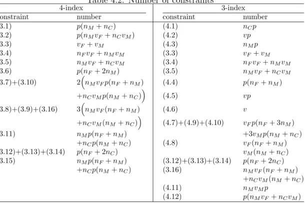
4.2 Number of constraints . . . 46
5.1 Differences of problem instances . . . 48
5.2 Time window tightness . . . 48
5.3 Performance of the valid inequalities . . . 50
5.4 Performance of the two-combination of valid inequalities (Part 1 ) 51 5.5 Performance of the two-combination of valid inequalities (Part 2 ) 52 5.6 Performance of the two-combination of valid inequalities (Part 3 ) 53 5.7 Performance of the valid inequalities . . . 54
5.8 Performance of the valid inequalities . . . 54
5.9 Performance of the valid inequalities . . . 56
5.10 Performance of the two-combination of valid inequalities . . . 57
5.11 Performance of the three-combination of valid inequalities . . . . 58
5.12 Performance of the three-combination of valid inequalities . . . . 59
5.13 Performance of the three-combination of valid inequalities . . . . 60
5.14 Performance of the valid inequalities . . . 61
5.15 Performance of the valid inequalities . . . 62
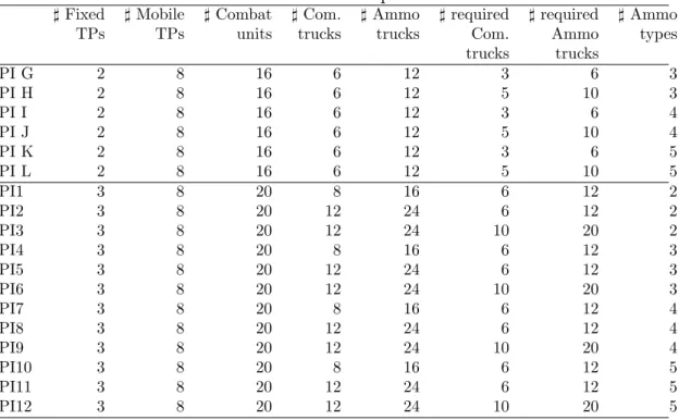
6.1 Characteristics of problem instances . . . 65
6.2 Gaps (%) and costs in 1 hour (small instances) . . . 70
6.3 Results of the base scenario . . . 72
6.4 Gaps of the problem instances with 4-index model and with the first objective . . . 76
6.5 Costs of the problem instances with 4-index model and with the first objective . . . 77
6.6 Gaps of the problem instances with 4-index model and with the second objective . . . 78
6.7 Costs of the problem instances with 4-index model and with the second objective . . . 79
6.8 Gaps of the problem instances with 3-index model and with the second objective . . . 81
6.9 Costs of the problem instances with 3-index model and with the
second objective . . . 82
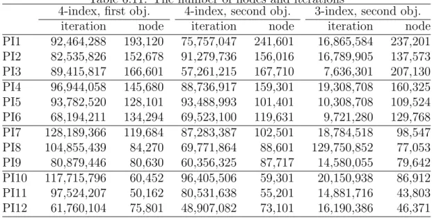
6.10 Summary of the problem instances . . . 83
6.11 The number of nodes and iterations . . . 84
6.12 Linear programming bound of 4-index model with the first objective 85 6.13 Linear programming bound of 4-index model with the second ob-jective . . . 85
6.14 Linear programming bound of 3-index model with the second ob-jective . . . 86
6.15 Computational results of the 4-index and 3-index models . . . 89
8.1 Run times (seconds) of heuristic 1 with the first objective . . . 117
8.2 Run times (seconds) of the problem instances with heuristic 1 and with the second objective . . . 118
8.3 Run times (seconds) of heuristic 2 with the first objective . . . 120
8.4 Run times (seconds) of the problem instances with heuristic 2 and with the second objective . . . 121
8.5 Run times (seconds) of the problem instances with heuristic 1 and with the second objective . . . 123
8.6 Run times (seconds) of the problem instances with heuristic 2 and with the second objective . . . 124
8.7 Summary of 4-index model with the first objective . . . 125
8.8 4-index model cost structure with the first objective . . . 126
8.10 4-index model cost structure with the second objective . . . 127
8.11 Summary of 3-index model with the second objective . . . 128
8.12 3-index model cost structure with the second objective . . . 129
A.1 Sets . . . 159
A.2 Parameters . . . 160
A.3 Decision variables of the 4-index formulation . . . 160
Introduction and Motivation
A soldier on the battlefield will be; hungry without food, thirsty without water but dead without ammunition.
The success of any type of combat operation depends on the availability of ammunition (henceforth called ammo), because a combat unit can fight so long as it receives ammo in the proper quantity, when and where it is needed. Hence, ammo is the dominant factor in determining the outcome of combat and any failure to supply the required amount of ammo may result in tactical defeat.
Previously, land forces of most countries relied upon heavy forces that were equipped with large number of heavy weapons for their lethality. The more heavy weapons a land force has, the more fire power it has and the more lethal it is. However, when equipped with such numbers and types of weapons, land forces lose their ability to move fast, and they need to keep enormous ammo inventories stocked at huge depots. Hence, ammo distribution system of these land forces is designed to support a heavy and slow moving force. It usually consists of different types of various depots most of which are underground storage facilities, bunkers or fortified storage areas.
In general, this distribution system is a continuous replenishment system in
which ammo flows from 1st level depots to combat units. Ammo, which is
pro-duced or procured, is first received by 1st level depots. From there it is
trans-ported to 2nd level depots typically by rail networks. From 2nd level depots ammo
is shipped to 3rd level depots mostly by trucks and if possible by rail. Then
com-bat units draw their ammo requirements from 3rd level depots with their own
trucks. In general, this system is a push system from 1st level depots to 3rd level
depots and a pull system from 3rd level depots to combat units, i.e. it is pushed
down to 3rd level depots and pulled from there by combat units.
With the end of Cold War, most of these traditional heavy land forces have moved towards a smaller, more agile, deployable and lethal force. Such a force does not depend solely on its firepower, but also on its mobility. This character-istic enables newly structured forces to move further and faster on the battlefield. To supply such a fast moving force, an effective and efficient distribution system is needed.
Current distribution system of most countries’ land forces may face some problems in supporting newly structured agile forces in their variety of missions and rapidly changing combat environments. Therefore, as land forces of most countries change their structure, their ammo distribution systems should be con-verted to a more mobile and flexible distribution process to provide more effective support.
To realize this request for an effective and flexible support system, we propose Mobile Ammunition Distribution System (Mobile-ADS). Our main objective is to deliver ammo as close to the combat units as possible, and do this in a timely manner. To do so, we suggest Fixed Transfer Points (Fixed-TPs) and Mobile Transfer Points (Mobile-TPs), that – after proper positioning – will cease the need for the remaining depots. Fixed-TPs are either railheads where the rail network ends or suitable locations on rail network where ammo can be transported safely as far as possible on the battlefield. Ammo is transferred from trains to commercial trucks at Fixed-TPs. Mobile-TPs are mostly forward staging areas where ammo trucks or stocks of ammo are kept for a short period of time before being moved further forward to support front line combat units. They are located
as close to combat units as possible to provide the least supply time. Ammo is transferred from commercial trucks to ammo trucks at Mobile-TPs. With their small and mobile structure Mobile-TPs can support agile land forces by moving with them accordingly.
The rest of this dissertation is organized as follows: Chapter 2 describes Mobile-ADS design problem, reviews the related literature and compares the characteristics of our problem with those of the majority of the literature. Chap-ter 3 demonstrates the 4-index static arc-based product flow mixed integer pro-gramming formulation of the design problem and derives several valid inequalities to improve the solution time. Chapter 4 presents the static 3-index node-based product flow mixed integer programming formulation of the design problem and derives several valid inequalities. Chapter 5 analyzes the effectiveness of the valid inequalities for both 4-index and 3-index formulations in some test problem instances and determines the ones that help reduce the solution time of the mod-els. Chapter 6 tests the 4-index and 3-index formulations in several realistic size problem instances. Chapter 7 introduces two heuristic approaches of which the first is a ”VRP first-LRP second“ and the second is a ”LRP first-VRP second“ heuristic. Chapter 8 evaluates the performance of the two heuristics in the same realistic scenarios. Chapter 9 extends the static 4-index formulation over time and presents a dynamic formulation to cover entire battle duration. Chapter 10 discusses how the static model can assist in a multi-period combat operation, and also how it can help the logistics planners when faced with unplanned combat situations. Chapter 11 presents the summary and the conclusions.
Problem Definition and Related
Literature
In this chapter, we first define the Mobile-ADS design problem. We, then, develop a classification scheme with 17 problem characteristics and classify 78 articles from the literature. Next, we give the classification of the problem we study. Finally, we highlight how our Mobile-ADS design problem differs from the existing studies in the literature.
2.1
Problem definition
Mobile-ADS is a continuous replenishment and a true push system. Highest level depots are the first to receive ammo that is produced or procured. Ammo is then moved forward as far as possible with rail networks. Where and how far we can carry ammo depends on the available rail network structure. We will assume those locations, where the rail network ends (rail heads), as potential Fixed-TP locations.
Within the context of this study we do not analyze the flow from the highest level depots to Fixed-TPs. We assume that the required amount of ammo can
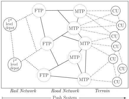
Rail Network Road Network Terrain FTP FTP FTP MTP MTP MTP MTP MTP CU 1st level depot 1st level depot CU CU CU CU CU CU Push System
Figure 2.1: Mobile ammo distribution system on the battlefield
be carried from the highest level depots to Fixed-TPs on time by rail. This assumption imposes no constraint on the system since there is enough ammo at the highest level depots and current rail network structure and equipment is sufficient to handle that amount.
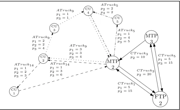
Ammo is moved from Fixed-TPs to Mobile-TPs by commercial trucks on road networks. Then Mobile-TPs issue ammo to their attached units with ammo trucks which have the capability to move on terrain and to load and unload themselves with their own crane. In such a system, combat units will not take the logistic burden of drawing their ammo by themselves, on the contrary, ammo will be pushed down to them. Figure 2.1 shows an example of a Mobile-ADS on the battlefield. Solid (dotted) circles represent fixed (potential) locations, respectively. Ammo is distributed from the highest level depots to Fixed-TPs (denoted by FTP in the figure) on rail networks by trains, from Fixed-TPs to Mobile-TPs (denoted by MTP in the figure) on road networks by commercial trucks, and from Mobile-TPs to combat units (denoted by CU in the figure) on terrain by ammo trucks.
In order to model Mobile-ADS we will take a snapshot of the battlefield and freeze the location of combat units at a particular point in time. Hence, the location of combat units will be fixed and the remaining decisions will be the locations of Fixed-TPs and Mobile-TPs in order to provide a bridge between the highest level depots and combat units.
A Mobile-TP can not be located anywhere on the battlefield. Such a site should possess characteristics to allow technical support operations as well as tactical defense against enemy threats. Logistics planners consider these char-acteristics and perform on-site or map reconnaissance to determine potential Mobile-TP locations before battle commences. As already explained, potential Fixed-TP locations are the rail heads that are close to battlefield.
In light of above explanations our problem is to supply combat units with correct types and quantities of ammo when and where it is needed. To do so, we need to consider the following planning requirements; (a) number and location of Fixed-TPs and Mobile-TPs, (b) vehicle routes and schedules to distribute ammo from Fixed-TPs to combat units via Mobile-TPs.
Solving above problems separately may lead to suboptimal decisions (see, for example, [75] for interdependency between location and routing). Therefore, these decisions must be made simultaneously. Hence, Mobile-ADS design prob-lem, which combines the location, routing and scheduling problems into a single model, is a Location Routing Problem (LRP).
2.2
Literature review
As stated in [59], LRPs solve the combined problem of (1) determining the opti-mal number and location of facilities that serve more than one demand point and (2) finding the optimal set of vehicle routes and schedules. In an LRP some loca-tion(s) must be decided among potential locations otherwise the problem becomes a sole routing problem. Likewise, tours must be allowed among facilities/demand points otherwise the problem would be reduced to a location problem.
If we follow the framework of [41] we can represent the distribution system in an LRP as layers. In this study, Fixed-TPs, Mobile-TPs and combat units exist at the first, second and third layers, respectively. Moreover, in this framework a tour is a round trip through several Mobile-TPs and/or combat units, making multiple deliveries.
There are several earlier studies that introduce LRP or review LRP literature, see for example [13], [41], [53], [59] and most recently [64]. An unpublished study, [1], also deserves considerable attention. In this study; authors review the LRP literature extensively including all problem variants (structure location or extensive facility location problems, etc.) according to a three-characteristic classification scheme: (1) deterministic or stochastic demand and supply, (2) central (pull type) or anticentral (push type) facilities and (3) single or multiple objectives. They explain some milestone studies that have longer lasting impact on LRP research, and state some untouched areas that require further study.
In [59] 12 (including solution methods) problem characteristics, and in [64] 9 (including solution methods) problem characteristics are used to classify the literature. Both classifications have 5 problem characteristics in common: (1) de-terministic or stochastic location-routing parameters (demand, supply size, etc.), (2) single or multiple facilities, (3) single or multiple periods and (4) single or multiple objectives (5) exact and heuristic methods ([59] investigates this char-acteristic separately).
In addition to above characteristics [59] has 7 distinct characteristics: (1) single-stage (only delivery routes) or two-stage (delivery and pick up routes), (2) single or multiple vehicles, (3) capacitated or uncapacitated vehicles, (4) capaci-tated or uncapacicapaci-tated facilities, (5) primary (origin or destination of a vehicle) or secondary (intermediate or transshipment node) facilities, (6) none or loose or strict time deadlines and (7) hypothetical or real data.
Likewise, [64] uses 4 distinct characteristics: (1) standard (no routes between facilities) or non-standard hierarchical structure, (2) exact or heuristic solution methods, (3) discrete or network or continuous solution space and (4) single or homogeneous or heterogeneous vehicle fleet.
While problem characteristics of [59] and [64] cover most of the key elements of the LRP framework, they do not fully address some elements that we believe are important. In addition, recent developments in logistics systems necessitate the alteration of some of their elements and employment of the new dimensions of distribution logistics into the classification. These alterations and additions of problem characteristics are described next.
A distribution system may consist of two layers (facilities and customers) or three/four layers (primary facilities, secondary facilities and customers). In todays just-in time environment a distribution system should address the time restrictions of customers. Customers may invoke no time restrictions (very un-likely), soft time restrictions (for example, one-sided time windows or time limits on driving times) or hard time restrictions (for example, two-sided time win-dows). Note that both loose and strict time deadlines of [59] are in the soft time restriction category. In a two-layer LRP (assuming customers are located at fixed and known locations at the second layer) we need to locate facilities at the first layer. In a three-layer LRP (with the same fixed customer location assumption at the third layer) we need to locate facilities at the first and/or second layers. In general, in a two or three/four-layer LRP locational decisions may exist at a single layer or at two different layers. LRPs may seek to distribute either a single product or multiple products. In an LRP with single sourcing each customer is to be supplied by exactly one vehicle or depot. On the contrary, customers may be supplied by more than one vehicle or depot which is referred to as multi sourcing. In an LRP there may exist inventories at the facilities that are to be located or there may not exist any inventory.
In light of above explanations we use a classification scheme consisting of 17 problem characteristics a summary of which is depicted in Table 2.1. Briefly, our classification shares the same 4 common characteristics with [59] and [64]: (1) deterministic or stochastic location-routing parameters (demand, supply size, etc.), (2) single or multiple facilities, (3) single or multiple periods and (4) single or multiple objectives.
Table 2.1: Classification scheme
1. Hierarchical level 7. Number of layers 13. Locational decision
a. Delivery or pickup a. Two a. At one layer
b. Delivery and pickup b. Three/Four b. At two layers
2. Nature of demand 8. Planning period 14. Product
a. Deterministic a. Single a. Single
b. Stochastic b. Multiple b. Multiple
3. Number of facilities 9. Time restriction 15. Sourcing
a. Single a. No a. Single
b. Multiple b. Soft b. Multiple
4. Vehicle fleet c. Hard 16. Inventory
a. Single 10. Objective function a. Exist
b. Homogeneous a. Single b. Not exist
c. Heterogeneous b. Multiple 17. Solution method
5. Vehicle capacity 11. Data a. Exact
a. Capacitated a. Real b. Heuristic
b. Uncapacitated b. Hypothetical
6. Facility capacity 12. Solution space
a. Capacitated a. Continuous
b. Uncapacitated b. Discrete
routes) or two-stage (delivery and pick up routes), (2) capacitated or uncapac-itated vehicles, (3) capacuncapac-itated or uncapacuncapac-itated facilities, (4) none or loose or strict time deadlines and (5) hypothetical or real data. Three of our characteris-tics exist in the classification of [64]: (1) exact or heuristic solution methods, (2) discrete or network or continuous solution space and (3) single or homogeneous or heterogeneous vehicle fleet.
In addition to above characteristics, we have 5 distinct characteristics that are not used by [59] or [64]: (1) two or three-four layers, (2) location at one layer or two layers, (3) single or multiple products, (4) single or multiple sourcing and (5) inventory exists or not exist.
We classify 78 studies according to the explained scheme. The details of our classification are presented in Tables 2.2 through 2.4 in chronological order.
T able 2.2: Classification of the literature (Part 1: A rticles fr om 1976 to 1989 ) 1 2 3 4 5 6 7 8 9 10 11 12 13 14 15 16 17 a b a b a b a b c a b a b a b a b a b c a b a b a b a b a b a b a b a b [22] X X X X X X X X X X X X X X X X X [26] X X X X X X X X X X X X X X X X X [27] X X X X X X X X X X X X X X X X X [35] X X X X X X X X X X X X X X X X X [67] X X X X X X X X X X X X X X X X X [37] X X X X X X X X X X X X X X X X X [44] X X X X X X X X X X X X X X X X X [65] X X X X X X X X X X X X X X X X X [46] X X X X X X X X X X X X X X X X X [56] X X X X X X X X X X X X X X X X X [70] X X X X X X X X X X X X X X X X X [39] X X X X X X X X X X X X X X X X X [71] X X X X X X X X X X X X X X X X X [14] X X X X X X X X X X X X X X X X X [45] X X X X X X X X X X X X X X X X X [15] X X X X X X X X X X X X X X X X X [18] X X X X X X X X X X X X X X X X X [47] X X X X X X X X X X X X X X X X X [81] X X X X X X X X X X X X X X X X X [16] X X X X X X X X X X X X X X X X X [42] X X X X X X X X X X X X X X X X X X [43] X X X X X X X X X X X X X X X X X [49] X X X X X X X X X X X X X X X X X [66] X X X X X X X X X X X X X X X X X X [89] X X X X X X X X X X X X X X X X X
T able 2.3: Classification of the literature (Part 2: A rticles fr om 1990 to 1999 ) 1 2 3 4 5 6 7 8 9 10 11 12 13 14 15 16 17 a b a b a b a b c a b a b a b a b a b c a b a b a b a b a b a b a b a b [19] X X X X X X X X X X X X X X X X X X [83] X X X X X X X X X X X X X X X X X [52] X X X X X X X X X X X X X X X X X [72] X X X X X X X X X X X X X X X X X [80] X X X X X X X X X X X X X X X X [29] X X X X X X X X X X X X X X X X X [78] X X X X X X X X X X X X X X X X X [82] X X X X X X X X X X X X X X X X X [84] X X X X X X X X X X X X X X X X X [8] X X X X X X X X X X X X X X X X X [10] X X X X X X X X X X X X X X X X X [34] X X X X X X X X X X X X X X X X X [36] X X X X X X X X X X X X X X X X X X [38] X X X X X X X X X X X X X X X X X [9] X X X X X X X X X X X X X X X X [13] X X X X X X X X X X X X X X X X X [21] X X X X X X X X X X X X X X X X X [77] X X X X X X X X X X X X X X X X X [58] X X X X X X X X X X X X X X X X X X [61] X X X X X X X X X X X X X X X X X [62] X X X X X X X X X X X X X X X X X [73] X X X X X X X X X X X X X X X X X [33] X X X X X X X X X X X X X X X X X [63] X X X X X X X X X X X X X X X X X [32] X X X X X X X X X X X X X X X X X [60] X X X X X X X X X X X X X X X X X [74] X X X X X X X X X X X X X X X X X [85] X X X X X X X X X X X X X X X X X
T able 2.4: Classification of the literature (Part 3: A rticles fr om 2000 to 2009 ) 1 2 3 4 5 6 7 8 9 10 11 12 13 14 15 16 17 a b a b a b a b c a b a b a b a b a b c a b a b a b a b a b a b a b a b [28] X X X X X X X X X X X X X X X X X [50] X X X X X X X X X X X X X X X X X [87] X X X X X X X X X X X X X X X X X [48] X X X X X X X X X X X X X X X X X [54] X X X X X X X X X X X X X X X X X [24] X X X X X X X X X X X X X X X X X [86] X X X X X X X X X X X X X X X X X [2] X X X X X X X X X X X X X X X X X [7] X X X X X X X X X X X X X X X X X [17] X X X X X X X X X X X X X X X X X [40] X X X X X X X X X X X X X X X X X X [57] X X X X X X X X X X X X X X X X X [3] X X X X X X X X X X X X X X X X X [76] X X X X X X X X X X X X X X X X X [51] X X X X X X X X X X X X X X X X X X [5] X X X X X X X X X X X X X X X X X [11] X X X X X X X X X X X X X X X X X X [23] X X X X X X X X X X X X X X X X X [68] X X X X X X X X X X X X X X X X X [4] X X X X X X X X X X X X X X X X X [79] X X X X X X X X X X X X X X X X X [88] X X X X X X X X X X X X X X X X X [12] X X X X X X X X X X X X X X X X X [30] X X X X X X X X X X X X X X X X X [6] X X X X X X X X X X X X X X X X X X
2.3
Comparison
To better reflect the characteristics of our Mobile-ADS design problem, to express where it stands in the LRP literature and to highlight how it distinguishes from the previous studies, we further explain some specifics pertaining to Mobile-ADS design problem and compare its classification with that of the majority of the LRP literature. The classification of Mobile-ADS design problem can be stated as follows:
• 1a. In Mobile-ADS we only consider the delivery of ammo to combat units. • 2a. All parameters (travel times, capacities, depot and transportation costs,
etc.) in the problem are assumed to be fixed and known. Here, the most problematic issue is daily ammo demand of combat units. Today, military services of almost all countries generally use three approaches to estimate the amount of ammo expected to be consumed daily (consumption rate) in combat. In the first method, we predict the number of targets a weapon will encounter on a daily basis, and multiply it with the required amount of ammo to destroy each target. In the second method, we predict the life of a weapon in combat before it is destroyed by enemy. Then, we predict the number of engagements in its lifetime, and multiply it with the expected ammo expenditure per engagement. In the third method, we use mathe-matical programming models. We define a combat scenario consisting of friendly and enemy weapons. We input several weapon and target charac-teristics, such as probability of hit, probability of kill, etc. Then the model gives the amount of ammo expended by each friendly weapon to defeat al-located enemy weapons. Most parameters used in these three methods (ex-pected target number, ex(ex-pected ammo expenditure per engagement, etc.) are based on historical data and actual field experiments or tests. However, they are constantly adjusted as new data is collected. In addition, to make the predictions more accurate, these parameters change depending on the type of mission (offense, defense, etc.), terrain (desert, forest, etc.), day of the combat (first day, second day, etc.) and anticipated operational tempo. Although, there is no visible way to predict daily requirements certainly
ahead of time, we are not totally in the dark either. Hence, we consider an-ticipated daily consumption rates, calculated as explained above, and treat them as fixed demands for the sake of our model’s tractability. Therefore, we assume that demand is fixed and known. Hence, Mobile-ADS design problem is a deterministic LRP.
• 3b. We locate multiple fixed and mobile transfer points.
• 4c. We have two different groups of vehicles, namely commercial and ammo
trucks. In addition, in each group we have various types of trucks that have different capacities which in turn have different acquisition and operation costs. For example, there exist 20, 30 and 40-ton commercial trucks and 5, 8 and 10-ton ammo trucks.
• 5a. Both commercial and ammo trucks are capacitated.
• 6a. Due to man power, terrain, enemy threat and fire safety considerations,
all transfer points have capacities.
• 7b. Three layers exist and Fixed-TPs/Mobile-TPs/combat units are located
at the first/second/third layers, respectively.
• 8ab. The problem of designing Mobile-ADS is very complex if we want
to capture all realities at once. Hence, to be able to better explain the problem and its formulation, we introduce the following limitation. Since battles generally continue for days, weeks or months, we need to consider several consecutive planning periods in our problem. However, due to the complexity, the dynamic version of the problem is presented following the consideration of the single planning period. Overall, we consider consecutive 24-hour planning periods since each combat unit possesses a specific amount of ammo on hand to initiate and continue combat operations for 24 hours until it is supplied from the rear.
• 9c. Battlefield is open to unexpected circumstances. At different times
of combat, depending on the combat type and enemy threat, some ammo types may become more valuable and combat units may require them more urgently than other types of ammo. Therefore, there are different time
deadlines for each type of ammo and for each combat unit. Not supplying a unit by this deadline with the necessary ammo means the unit continues combat without the required ammo type – a potentially lethal situation for a unit engaged with the enemy in combat – between the unit’s time deadline and the supply time. In addition, as combat continues, units change their locations and resupply becomes even more difficult. Supplying a unit with ammo requires the unit to halt for some time and take the required precautions such as perimeter security, etc. A combat unit can not always halt in battle especially when it is actively engaged with the enemy. Hence, after combat starts, units need some time to gain a position that renders them available for supply and this time constitutes the earliest time that a unit can be supplied. In summary, we have two-sided time windows, i.e. hard time restrictions in our problem.
• 10a. Total Mobile-ADS cost consists of three separate components, namely,
fixed cost of opening transfer points, acquisition cost of vehicle fleet and transportation cost of ammo. Hence, we have a single objective function that unifies multiple cost components.
• 11b. Since this is a military application on a sensitive topic all data we
present in this dissertation is hypothetical.
• 12b. As already explained, before battle starts, logistics planners
deter-mine potential locations for each type of transfer point on the battlefield. Therefore, transfer points can only be located at these predefined potential locations and hence the solution space of our problem is discrete.
• 13b. In Mobile-ADS design problem our aim is to locate Fixed-TPs at the
first layer and Mobile-TPs at the second layer properly to supply combat units on time. Hence, locational decisions exist at two different layers in our problem.
• 14b. On the battlefield, combat units need and use several types of ammo.
They need them at different locations, in different times and at different rates. Therefore, in Mobile-ADS we distribute multiple ammo types.
• 15b. In an LRP with single sourcing, each customer is to be supplied by
exactly one vehicle or depot. In our problem, even the same ammo type may be brought to a unit by two or more different trucks. Hence, multi sourcing exists in our model.
• 16b. We do not hold inventory at transfer points.
• 17ab. We solve the model exactly by a commercial solver and heuristically
by two methods that are developed in this dissertation.
Table 2.5 summarizes the classification of the 78 studies we examined and compares the classification of the proposed Mobile-ADS design problem with that of the majority of the literature. We utilize a capacitated heterogeneous vehicle fleet whereas the studies in the literature generally use capacitated homogeneous fleet. Majority of the previous studies consider uncapacitated facilities but we consider capacitated ones. In the literature majority of the models are two layers whereas Mobile-ADS has three layers.
T able 2.5: Summary of LRP studies 1. Hierarc hical lev el 7. Num b er of la yers 13. Lo cational decision a. Deliv ery or pic kup 73 a. Tw o 61 a. A t one la yer 75 b. Deliv ery and pic kup 5 b. Three/F our 17 b. A t tw o la yers 3 2. Nature of demand 8. Planning p erio d 14. Pro duct a. Deterministic 61 a. Single 72 a. Single 74 b. Sto chastic 17 b. Multiple 7 b. Multiple 4 3. Num b er of facilities 9. Time restriction 15. Sourcing a. Single 19 a. No 63 a. Single 77 b. Multiple 59 b. Soft 14 b. Multiple 1 4. V ehicle fleet c. Hard 1 16. In ven tory a. Single 12 10. Ob jectiv e function a. Exist 4 b. Homogeneous 52 a. Single 72 b. Not exist 74 c. Heterogeneous 14 b. Multiple 7 17. Solution metho d 5. V ehicle capacit y 11. Data a. Exact 25 a. Capacitated 47 a. Real 23 b. Heuristic 55 b. Uncapacitated 31 b. Hyp othetical 57 6. F acilit y capacit y 12. Solution space a. Capacitated 31 a. Con tin uous 4 b. Uncapacitated 48 b. Discrete 74 Majority : 1a, 2a, 3b, 4b, 5a, 6b, 7a, 8a, 9a, 10a, 11b, 12b, 13a, 14a, 15a, 16b, 17b. Mobile-ADS : 1a, 2a, 3b, 4c, 5a, 6a, 7b, 8a,b, 9c, 10a, 11b, 12b, 13b, 14b, 15b, 16b, 17a,b.
Except for 7 studies, the literature solve static LRP problems, while we solve both a single-period static and a multi-period dynamic case. Time restriction issue is rarely incorporated within the context of LRP models in the literature. 14 studies include soft time restrictions and only one study (time windows are used in [78] however no mathematical formulation is given) includes hard time restrictions. We utilize hard time restrictions in Mobile-ADS design problem. Locational decisions exist at only one layer in all studies except three. In other words, almost all three layer models locate facilities only at the second layer and facility locations at the first layer are assumed to be known a priori. We locate facilities at two different layers.
To the best of our knowledge, there are only 4 studies that distribute multiple products and the rest deals with single product. However, single-product formu-lations can hardly help model complex real world distribution systems with many number of types of products to be distributed. In Mobile-ADS design problem we distribute multiple products. Last of all, except one study all previous mod-els compel single sourcing and no study allows multiple sourcing (a customer is allowed to be served by at most two vehicles in the model of [63], but one for pickups and one for deliveries). We utilize multiple sourcing which may help to reach better solutions in large distribution systems.
This brief analysis illustrates that some characteristics of the Mobile-ADS design problem are rarely included in the previous models. This dissertation is aimed directly to handle these aspects and to incorporate them into a single model. To the best of our knowledge this is the first attempt to construct such an inclusive real world LRP model.
Static 4-Index Model
Development
In this chapter we present the mathematical formulation of Mobile-ADS design problem for a fixed period and derive several valid inequalities to speed up the solution time.
We model the battlefield as a network of three types of nodes, i.e. potential Fixed-TP and Mobile-TP locations and fixed combat unit locations. With this representation we consider the Mobile-ADS, shown in Figure 2.1, as a directed and connected network G = (N, A) that is defined by a set N of nodes and a set A of arcs. N is partitioned into three mutually exclusive subsets such that
N = NF
S
NM
S
NC where NF (NM) is the set of potential Fixed-TP
(Mobile-TP) locations respectively and NC is the set of combat unit locations. Moreover,
we let NF M = NF
S
NM and NM C = NM
S
NC. A consists of two types of
road networks that is A = A1
S
A2. A1 is the two-way road network, on which
commercial trucks can travel between Fixed-TPs and Mobile-TPs and among Mobile-TPs. A2 is the two-way trace network on the battle terrain, on which
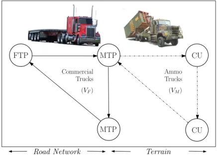
ammo trucks can travel between Mobile-TPs and combat units and among combat units. Figure 3.1 shows an example of a route of a commercial and ammo truck.
V is the set of all vehicles consisting of two subsets, V = VF
S
VM, where VF
Road Network Terrain MTP MTP FTP CU CU (VF) Trucks Commercial Trucks Ammo (VM)
Figure 3.1: Routes of commercial and special ammo trucks
is the set of commercial trucks that are stationed at Fixed-TPs, and VM is the
set of ammo trucks that are stationed at Mobile-TPs. P is the ammo type set.
D = [Dij] is the distance matrix where the distance Dij between two nodes
i and j is the length of the shortest path from i to j on G. We assume that
the matrix D of shortest distances is known in advance. We also assume that all travel on G occur on the shortest paths and at two different constant speeds.
speedc and speeda denote the constant speeds of commercial and ammo trucks,
respectively where speedc > speeda. Then T = [T Iij] is the travel time matrix
where (1) if i ∈ NF and j ∈ NM or i, j ∈ NM, i 6= j then T Iij = Dij/speedc and
(2) if i ∈ NM and j ∈ NC or i, j ∈ NC, i 6= j then T Iij = Dij/speeda.
We also present all sets, parameters and decision variables that are used throughout this study in the Appendix.
We introduce a 4-index commodity flow mixed integer programming formu-lation for the Mobile-ADS design problem. Note that only the nonnegative com-modity flow variable has 4 indices and all binary variables have three or less indices. We use the following parameters in the formulation. Qip is the demand
of combat unit i for ammo type p. Each transfer point i has a nonnegative ca-pacity represented by CDip for ammo type p. Each vehicle v has a nonnegative
capacity CVvp for ammo type p and in addition all vehicles also have total
capac-ities represented by CTv. As explained above there are different time deadlines
for each type of ammo and for each combat unit and each unit has a different earliest time after which that unit can be supplied. T Eip is the earliest and T Lip
is the latest time that combat unit i be supplied with ammo type p. T Mp is
the maximum latest arrival time of ammo type p among combat units, that is
T Mp = maxi∈NC{T Lip}. T M = maxp∈P{T Mp} represents the maximum of the
latest arrival times of all ammo types. T Cvp is the cost of transporting one unit
of ammo type p on vehicle v per hour. V Cv is the cost of acquiring vehicle v.
F Ci is the fixed cost of establishing/opening transfer point i.
The Mobile-ADS design problem can be summarized as follows. We have a fi-nite number of combat units engaged with enemy on the battlefield. We also have a finite set of potential Fixed-TP and potential Mobile-TP locations (two sets are disjoint). Ammo flows from Fixed-TPs to Mobile-TPs by commercial trucks and from Mobile-TPs to combat units by special ammo trucks. We have to decide on (1) the number and location of Fixed-TPs and Mobile-TPs to be established and (2) the number, home transfer point and route of commercial and ammo trucks to serve combat units while minimizing transfer point establishment, truck ac-quisition and ammo transportation costs, such that the following conditions are satisfied;
• Total demand of combat units is satisfied within the given time window, • Transfer point and truck capacity restrictions are respected,
• Each commercial (ammo) truck is dispatched from its home transfer point
and returns to that point after serving the Mobile-TPs (combat units) on its route,
3.1
Constraints
We employ the following notational rules throughout the formulation. We enu-merate separate constraints as usual such as 3.1, 3.2, ... If we write the same constraint several times for disjoint index sets then we enumerate them such as 3.1a, 3.1b, ... or 3.2a, 3.2b, ... and so on.
3.1.1
Product flow balance constraints
We use nonnegative decision variable fijvp to denote the amount of flow of ammo
type p carried from node i to node j by vehicle v.
X v∈VF µ X j∈NF M j6=i fjivp− X j∈NM j6=i fijvp ¶ = X v∈VM X j∈NC
fijvp ∀i ∈ NM, p ∈ P (3.1a)
X v∈VM µ X j∈NM C j6=i fjivp− X j∈NC j6=i fijvp ¶ = Qip ∀i ∈ NC, p ∈ P (3.1b) X j∈NF M j6=i fjivp ≥ X j∈NM j6=i
fijvp ∀i ∈ NM, v ∈ VF, p ∈ P (3.2a)
X j∈NM C j6=i fjivp ≥ X j∈NC j6=i fijvp ∀i ∈ NC, v ∈ VM, p ∈ P (3.2b)
Ammo enters the network from Fixed-TPs and it is consumed by combat units. Constraints (3.1) ensure that inflow to a Mobile-TP or combat unit is equal to the sum of the total outflow from that node and the demand of that node. Constraints (3.2) guarantee that vehicles can not pick up ammo at intermediate nodes on their routes by forcing that a vehicle does not leave a node with more amount of an ammo type than the amount it was carrying while it was entering that node.
Note that constraints (3.1b) declare the problem infeasible if the total demand can not be satisfied for some reason, such as lack of ammo or trucks or transfer points, tight time windows, etc. In such situations, instead of giving no solution, we may want to provide the best solution that can be obtained with available resources. To do so, we need to allow the demand satisfaction limitation to be overruled at a certain cost by rewriting hard constraints (3.1b) as soft constraints as follows Pv∈VM µ P j∈NM C j6=i fjivp− P j∈NC j6=i fijvp ¶ + uip = Qip where uip is a
non-negative decision variable, indicating the amount of unmet demand of ammo type
p at combat unit i, with a high enough positive cost coefficient in the objective
function.
3.1.2
Vehicle flow balance constraints
We use binary decision variable xijv, where xijv = 1 if vehicle v travels from node
i to node j and xijv = 0 otherwise.
X i∈NF X j∈NM xijv ≤ 1 ∀v ∈ VF (3.3a) X i∈NM X j∈NC xijv ≤ 1 ∀v ∈ VM (3.3b) X j∈NM xjiv = X j∈NM
xijv ∀i ∈ NF, v ∈ VF (3.4a)
X j∈NC xjiv = X j∈NC xijv ∀i ∈ NM, v ∈ VM (3.4b) X j∈NF M j6=i xjiv = X j∈NF M j6=i
xijv ∀i ∈ NM, v ∈ VF (3.5a)
X j∈NM C j6=i xjiv = X j∈NM C j6=i xijv ∀i ∈ NC, v ∈ VM (3.5b)
Recall that commercial trucks can be allocated only to Fixed-TPs and ammo trucks only to Mobile-TPs. Constraints (3.3) indicate that a vehicle can not be allocated to more than one transfer point. From another point of view, they maintain that a vehicle can start its route from one and only one transfer point. Constraints (3.4) force each vehicle to turn back to its home transfer point where it is allocated. Constraints (3.5) require that each vehicle leaves the node that it enters. Constraints (3.3)-(3.5) together also maintain that each route contains only one transfer point and they guarantee that a vehicle can not go from a node to two or more nodes at the same time.
3.1.3
Capacity constraints
We use binary decision variable yi, where yi = 1 if transfer point i is established
and yi = 0 otherwise.
X
v∈VF
X
j∈NM
fijvp ≤ CDip· yi ∀i ∈ NF, p ∈ P (3.6a)
X v∈VM X j∈NC fijvp ≤ CDip· yi ∀i ∈ NM, p ∈ P (3.6b) X v∈VF X j∈NM j6=i fijvp ≤ µ X l∈NC Qlp ¶ · yi ∀i ∈ NM, p ∈ P (3.6c)
fijvp ≤ CVvp· xijv ∀i ∈ NF, j ∈ NM, v ∈ VF, p ∈ P (3.7)
∀i, j ∈ NM, i 6= j, v ∈ VF, p ∈ P
∀i ∈ NM, j ∈ NC, v ∈ VM, p ∈ P
∀i, j ∈ NC, i 6= j, v ∈ VM, p ∈ P
X
p∈P
fijvp ≤ CTv· xijv ∀i ∈ NF, j ∈ NM, v ∈ VF (3.8)
∀i, j ∈ NM, i 6= j, v ∈ VF
∀i, j ∈ NC, i 6= j, v ∈ VM
Constraints (3.6) ensure that transfer points can not send/receive ammo type
p more than their capacity for that ammo type. They also guarantee that there
is no flow from/through any closed transfer point. Constraints (3.7) require that vehicle capacities are not exceeded and maintain that unused vehicles can not carry any flow. All vehicles also have total capacities that are respected by constraints (3.8).
3.1.4
Relation constraints
We use binary decision variable wijp, where wijp= 1 if ammo type p travels from
node i to node j and wijp= 0 otherwise.
X
p∈P
fijvp ≥ xijv ∀i ∈ NF, j ∈ NM, v ∈ VF (3.9)
∀i, j ∈ NM, i 6= j, v ∈ VF ∀i ∈ NM, j ∈ NC, v ∈ VM ∀i, j ∈ NC, i 6= j, v ∈ VM µ X l∈NC Qlp 
· wijp≥ fijvp ∀i ∈ NF, j ∈ NM, v ∈ VF, p ∈ P (3.10)
∀i, j ∈ NM, i 6= j, v ∈ VF, p ∈ P
∀i ∈ NM, j ∈ NC, v ∈ VM, p ∈ P
∀i, j ∈ NC, i 6= j, v ∈ VM, p ∈ P
X
v∈VF
fijvp ≥ wijp ∀i ∈ NF, j ∈ NM, p ∈ P (3.11a)
X
v∈VM
fijvp ≥ wijp ∀i ∈ NM, j ∈ NC, p ∈ P (3.11b)
∀i, j ∈ NC, i 6= j, p ∈ P
Constraints (3.9) require that a vehicle carries some type and amount of ammo if it is dispatched. Note that these constraints do not force vehicles to carry ammo on their way back to their home transfer points. They also guarantee that if a vehicle does not carry anything from node i to node j then it should not travel between these two nodes. Constraints (3.10) and (3.11) set the correct logical relationships between the decision variables f and w. They maintain that if ammo type p does not travel between nodes i and j then no flow of p should exist between these nodes and reversely if ammo type p does travel from i to j then there must exist some positive flow of p in between.
Note that in constraints (3.9) and (3.11), ammo flow is measured in undefined units. Hence, one needs to be careful about defining the unit of flow, because these constraints do not permit a truck to carry an ammo type less than 1 unit. If one wants to do so, then the right hand sides should be multiplied with an appropriate multiplier. For example, if our unit is 1 ton, and if we do not want to carry an ammo type less than 0.2 tons with a single truck, then our multiplier would be 0.2.
3.1.5
Time related constraints
We use nonnegative decision variable tpipto denote the arrival time of ammo type
p at node i.
tpip ≥ T Eip ∀i ∈ NC, p ∈ P (3.12)
tpip ≤ T Lip ∀i ∈ NC, p ∈ P (3.13)
tpip = 0 ∀i ∈ NF, p ∈ P (3.14)
∀i, j ∈ NM, i 6= j, p ∈ P
∀i ∈ NM, j ∈ NC, p ∈ P
∀i, j ∈ NC, i 6= j, p ∈ P
Constraints (3.12) and (3.13) impose the time window requirements of combat units on the model for all ammo types. Constraints (3.14) define the initial condition by setting the arrival time of all ammo types at Fixed-TPs to time zero. Constraints (3.15) compute the arrival times of ammo types at nodes.
In fact, since constraints (3.15) refer to the latest ammo arrival, constraints (3.12) ensure that the latest ammo arrival respects the time windows of units. Note that waiting of ammo at combat units is allowed, and in the context of this dissertation, a time window indicates the time interval in which a unit can halt in battle, and receive the waiting or newly arrived supplies. Hence, ammo is allowed to reach a unit before the earliest time, and wait there until the unit actually takes it.
Recall that the decision variable wijp does not carry any information about
vehicles. Hence constraints (3.12)-(3.15), which are written for wijp’s, can not
prevent sub-tours of vehicles. To remedy this condition we introduce subtour elimination constraints of [25] as constraints (3.16). Note that we use nonnegative decision variable tviv to denote the arrival time of vehicle v at node i.
tviv+ T Iij · xijv − T M · (1 − xijv) ≤ tvjv ∀i ∈ NF, j ∈ NM, v ∈ VF (3.16)
∀i, j ∈ NM, i 6= j, v ∈ VF
∀i ∈ NM, j ∈ NC, v ∈ VM
3.2
Objective function
In Mobile-ADS design problem two different objectives exists each of which could be applicable depending on the situation. The first objective considers the costs of transfer point establishment, vehicle acquisition, and ammo distribution. The second one considers again the costs of transfer point establishment and vehi-cle acquisition plus the cost of truck driving. As can be seen, two of the cost components are common to both objectives and are shown below.
X i∈NF M F Ci· yi (3.17) X i∈NF X j∈NM X v∈VF V Cv · xijv+ X i∈NM X j∈NC X v∈VM V Cv· xijv (3.18)
(3.17) is the total fixed cost of opening transfer points, and (3.18) is the total acquisition cost of used trucks. Now, we present the last component of each objective.
Depending on the mission, available forces, enemy threat, country’s economy, etc. different factors may gain more importance or urgency above others on the battlefield. If we put economy and financial concerns over others, then total transportation cost of ammo becomes critical. This cost constitutes the third component of the first objective and is shown below.
X i∈N X j∈N X v∈V X p∈P T Cvp· T Iij · fijvp (3.19)
If enemy has the ability to detect our logistics convoys, then the more traffic we have the more our convoys are exposed to enemy fire. Moreover, we may want to concentrate some of our forces on a particular region of the combat area without enemy’s notice. In such circumstances, stealth becomes a big concern, and we again do not want much traffic on the battlefield. Hence, total driving time of vehicles becomes critical, and constitutes the third component of the second objective that is shown below.
X i∈N X j∈N X v∈V DCv· T Iij · xijv (3.20)
To summarize, our objective functions are as follows.
• z1 = (3.17) + (3.18) + (3.19) • z2 = (3.17) + (3.18) + (3.20)
It is important to note that on the same battlefield and at the same time, different objectives may gain priority for different units. For example, one brigade may move to a different direction in concealment while others keep their positions as they are. Hence, for the first brigade z2 and for the rest z1 may become the objective on the same battlefield at the same time.
3.3
Model
In light of above explanations Mobile-ADS design model is,
min z1 or z2 s.t. (3.1) − (3.16) fijvp ≥ 0 ∀i, j ∈ N, i 6= j, v ∈ V, p ∈ P tpip ≥ 0 ∀i ∈ N, p ∈ P tviv≥ 0 ∀i ∈ N, v ∈ V xijv ∈ {0, 1} ∀i, j ∈ N, i 6= j, v ∈ V wijp∈ {0, 1} ∀i, j ∈ N, i 6= j, p ∈ P yi ∈ {0, 1} ∀i ∈ NF M.
3.4
Valid inequalities
We model the Mobile-ADS design problem as a mixed integer programming model. In this section we present several valid inequalities to improve its perfor-mance in terms of solution time and quality.
3.4.1
Valid inequalities related to product flow balance
X v∈VF X i∈NF X j∈NM fijvp = X i∈NC Qip ∀p ∈ P (V 1a) X v∈VM X i∈NM X j∈NC fijvp = X i∈NC Qip ∀p ∈ P (V 1b)Valid inequalities (V 1) require that outflow from all Fixed-TPs and from all Mobile-TPs be equal to the total demand of all combat units for each ammo type.
3.4.2
Valid inequalities related to vehicle flow balance
X
j∈NF M
j6=i
xijv ≤ 1 ∀i ∈ NM, v ∈ VF (V 2a)
X j∈NM C j6=i xijv ≤ 1 ∀i ∈ NC, v ∈ VM (V 2b) X v∈VF X i∈NF X j∈NM xijv ≥ »P p∈P P i∈NCQip maxv∈VF{CTv} ¼ (V 3a) X v∈VM X i∈NM X j∈NC xijv ≥ »P p∈P P i∈NCQip maxv∈VM{CTv} ¼ (V 3b)
Valid inequalities (V 2) maintain that a vehicle can not travel from a node to two or more nodes in a single planning period. Valid inequalities (V 3) set a lower bound for the total number of vehicles that must be dispatched from transfer points to carry the total demand of all combat units.
3.4.3
Valid inequalities related to variable and logical
re-lations
wijp≤ yi ∀i ∈ NF, j ∈ NM, p ∈ P (V 4) ∀i, j ∈ NM, i 6= j, p ∈ P ∀i ∈ NM, j ∈ NC, p ∈ P X p∈P X j∈NMwijp ≥ yi ∀i ∈ NF (V 5a)
X
p∈P
X
j∈NC
wijp ≥ yi ∀i ∈ NM (V 5b)
Valid inequalities (V 4) ensure that ammo types can not pass through closed transfer points. Valid inequalities (V 5) provide that at least one ammo type must pass through an open transfer point.
wijp≤
X
v∈VF
xijv ∀i ∈ NF, j ∈ NM, p ∈ P (V 6a)
∀i, j ∈ NM, i 6= j, p ∈ P wijp≤ X v∈VM xijv ∀i ∈ NM, j ∈ NC, p ∈ P (V 6b) ∀i, j ∈ NC, i 6= j, p ∈ P X p∈P
wijp≥ xijv ∀i ∈ NF, j ∈ NM, v ∈ VF (V 7)
∀i, j ∈ NM, i 6= j, v ∈ VF
∀i ∈ NM, j ∈ NC, v ∈ VM
Valid inequalities (V 6) state that if an ammo type travels from node i to node
j then there must exist at least one vehicle travelling between these two nodes.
Valid inequalities (V 7) maintain the reverse condition by preventing any vehicle from traveling between nodes i and j if no ammo type travels between these two nodes.
X
j∈NM
xijv ≤ yi ∀i ∈ NF, v ∈ VF (V 8a)
X j∈NF M j6=i xijv ≤ yi ∀i ∈ NM, v ∈ VF (V 8b) X j∈NC xijv ≤ yi ∀i ∈ NM, v ∈ VM (V 8c) X v∈VF X j∈NM
xijv ≥ yi ∀i ∈ NF (V 9a)
X v∈VM X j∈NC xijv ≥ yi ∀i ∈ NM (V 9b) X v∈VF X j∈NM
xijv ≤ |VF| · yi ∀i ∈ NF (V 10a)
X
v∈VM
X
j∈NC
xijv ≤ |VM| · yi ∀i ∈ NM (V 10b)
Valid inequalities (V 8) provide that no vehicle can be dispatched from or pass through a closed transfer point. Valid inequalities (V 9) require that an open transfer point must dispatch at least one vehicle. Valid inequalities (V 10) guarantee that no transfer point can dispatch more vehicles than there exist in the system. X i∈NF yi ≤ |NF| (V 11a) X i∈NM yi ≤ |NM| (V 11b)
X i∈NF yi ≥ » P p∈P P i∈NCQip maxp∈P,i∈NF{CDip} ¼ (V 12a) X i∈NM yi ≥ » P p∈P P i∈NCQip maxp∈P,i∈NM{CDip} ¼ (V 12b)
Valid inequalities (V 11) and (V 12) set the upper and lower bounds for the number of opened transfer points.
3.4.4
Valid inequalities related to time
X i∈NM C i6=j X j∈NC T Iij · xijv ≤ T M − min i∈NF,j∈NM {T Iij} ∀v ∈ VM (V 13)
Consider the tours of ammo trucks an example of which can be seen in Figure 3.1 and consider deleting the returning arc of each tour from combat units to Mobile-TPs. Valid inequalities (V 13) set the upper bound for the total traveling time of these modified routes of ammo trucks. The total traveling time of the modified route of ammo truck v is represented byPi∈NM C
i6=j
P
j∈NCT Iij·xijv. In fact
this summation also defines the serving time of the last combat unit on the tour of ammo truck v. Now, let the maximum of the latest arrival times of all ammo types at combat units be 24, that is T M = 24. In other words, all ammo types must be delivered to combat units in 24 hours. Suppose, minimum traveling time between Fixed-TPs and Mobile-TPs is 7, that is mini∈NF,j∈NM{T Iij} = 7. Hence,
the earliest time that a Mobile-TP can dispatch an ammo truck is 7. However, all ammo types must arrive at combat units before 24. Combining these two observations, all ammo trucks have at most 14 hours to serve all combat units. Mathematically, we havePi∈NM C
i6=j
P
j∈NCT Iij·xijv ≤ 14 meaning that each ammo
truck should deliver the demand of the last combat unit on its tour in at most 14 hours.
Static 3-Index Model
Development
In Chapter 3 we present a 4-index mathematical formulation of Mobile-ADS design problem with an arc-based product flow approach. In this chapter we develop a 3-index mathematical formulation of the same problem with a node-based product flow approach.
As in the 4-index model, we still have the same directed and connected network
G = (N, A) with N = NF S NM S NC and A = A1 S
A2. We also have the same
vehicle set V = VF
S
VM and travel time matrix T . In addition, we use the same
parameters as we did in the 4-index model. Finally, our problem definition and the answers we are expecting from the 3-index model are the same.
In the 4-index model we consider vehicle and product flows on the arcs of the network. We indicate the traversal of vehicle v ∈ V on arc (i, j) ∈ A using the binary decision variable xijv. We also denote the flow of product p ∈ P on arc
(i, j) ∈ A with vehicle v ∈ V by the positive decision variable fijvp.
In the 3-index model we still use the same indicator variables for vehicle traversals on arcs. However, rather than product flow on arcs we consider product flow on the nodes of the network. To do so, we consider the product flow on arc