Manoeuvring-target tracking with the Viterbi algorithm in the presence of interference

(1)

Manoeuvring-target tracking with the Viterbi

algorithm in the presence of interference

Kerim Demirbag

Indexing terms: Radar, Algorithms, Interference, Signal processing, Target tracking, Air traflc control

Abstract: The Viterbi algorithm is used to track a target in the presence of random interference, such as jamming. A nonlinear target motion and an observation which is modelled in a spherical co- ordinate system are considered. The observation model is a nonlinear function of interference. The components of the state vector are the range, bearing angle, and elevation angle of the target location. The state vector is estimated, component-by-component, by a parallel use of the Viterbi algorithm in blocks. Simulation results, some of which are presented, have shown that the proposed estimation scheme performs well, whereas classical estimation schemes, such as the extended Kalman filter, cannot, in general, handle target tracking in the presence of random interference.

model containing an arbitrary random interference and an observation noise, where the state vector is estimated as a vector.

Recently, Demirbag [2] has used multiple hypothesis testing to track a manoeuvring target, using an observation model which does not contain any random interference, i.e. contains only an observation noise. The state vector (whose components represent the range, bearing angle, and elevation angle) is estimated component-by- component. The tracking scheme used avoids the errors in the state estimate which result from the model linear- isation [6] required by the use of the extended Kalman filter to track a target, since the scheme presented in Ref- erence 2 does not require any model linearisation.

In this paper, the scheme for manoeuvring-target tracking, as proposed by Demirbag [2], is extended to the case where an observation contains an arbitrary nonlinear random interference as well as an observation noise.

1 Introduction

Manoeuvring-target tracking with the (extended) Kalman filter has been extensively considered in the literature. The use of the (extended) Kalman filter requires an observation model containing only an additive white noise. If the noise is not additive, then the (extended) Kalman filter cannot be used for target tracking unless the observation model is approximated by a model containing an additive white noise [4].

In target tracking in the presence of random interference, an observation contains an observation noise and also a random interference, such as jamming, which can arbitrarily affect the observation. Hence, the observation in the presence of interference may be modelled by a nonlinear function of the interference. In this case, classical estimation techniques, such as the (extended) Kalman filter, may not be used to estimate the states of the target motion due to nonlinear interference contained in the observation [4]. If the classical estimation schemes were used by assuming zero interference, the state estimates would diverge from the actual state values [l].

State estimation with an observation model containing an additive white observation noise and a Markov chain, which may represent the interference, has been considered in the literature [lo, 111. Moreover, Demirbag

[ 11 has considered state estimation with an observation

Paper 6837F (E15), first received 5th October 1988 and in revised form 26th June 1989

The author is with the Department of Electrical Engineering and Com- puter Science (M/C 154), University of Illinois at Chicago, PO BOX 4348, Chicago, IL 60680, USA

The work reported in this paper was camed out while the author was visiting Bilkent University, Ankara, Turkey

262

2 Statement of the problem

In this paper, the motion of a manoeuvring target is assumed to be described by the nonlinear models for range, bearing angle, and elevation angle which are derived in Reference 2 and stated in Section 7.1.

Let x(k)T = [x,(k), x,(k), x3(k)] be the transpose of the state vector whose components x,(k), x2(k) and x3(k) rep- resent the range, bearing angle and elevation angle of the target location at time k, respectively. Throughout this paper, the superscript T indicates the transpose, and boldface letters denote vectors. The model of each state component, say the ith state component, is given by

xXk

+

1) 4 fiCU(k), xi(k), xLkL xXkL f(k), w(k)I (1) where i # j # 1 and i, j , 1 E [l, 2, 31, and the subscript i

denotes the component label; w(k)T = [w,(k), w,(k), w3(k)] is a zero-mean disturbance noise vector wlth

known statistics; ~ ( k ) ~ = [u,(k), u,(k), U&)] is a known

deterministic pilot command vector whose components u,(k), u2(k) and u3(k) affect the target motion at time k in the range, bearing angle, and elevation angle directions, respectively; f(k) is the derivative of the state vector x(k)

with respect to time;fi[.

.

.] is a nonlinear function whose explicit expression is given in Section 6.1. This function defines the ith state component at time k

+

1 in terms of the pilot command vector, disturbance noise vector, state vector, and derivative of the state vector at time k. The function

fi[.

.

.] is sometimes referred to as the ith state component defining-function or the ith state component model of the target motion in the spherical co-ordinate system.

In target tracking in the presence of random interference, observations (which are made by a radar in a spherical co-ordinate system) contain an observation

(2)

noise and also an arbitrary random interference. This interference can represent jamming or any other random phenomena (except for the observation noise) affecting the observation. If there were no interference, the observation model for each state component would be a linear function of this state component and an observation noise [SI. However, in the presence of interference, the observation for each state component can be a nonlinear function of interference. This paper assumes that the observation for the ith state component is a nonlinear function of the ith state component, and of the interference and observation noise affecting the observation. This is the case in practice. As an example, consider the observation taken by a radar for the range. This is a function of only the range, of the interference (e.g. jamming) affecting the range, and of the observation noise. Hence in this paper the observation model for the ith state component is assumed to be given by

zXk) = giCxi(k), Zdk), ~ i ( k l l i = 1,293 (2) where s i [

...I

is a given nonlinear function of xXk), Zdk)

and oik). z,(k), z2(k) and z3(k) are the observations; Zl(k),

Z2(k) and Z,(k) are interference vectors with known sta-

tistics; and u,(k), u,(k) and U&) are the observation

noises with known statistics in the range, bearing angle, and elevation angle directions, respectively. It is also assumed that the initial state vector and all samples of the interferences, and disturbance and observation noises are independent.

It is of interest to estimate the state component sequences

X i = {xdo), xi(1),

...,

xAk), ...} by using the observation sequence

Zi = {zi(l), zi(2), ..., zi(k), ..}

i = 1, 2, 3

i = 1, 2, 3 This is discussed next.

3 Estimation scheme

State vector x( .) is estimated in blocks. Without loss of generality, each block is assumed to have a length of B,

except for the first block which has a length of B

+

1. In a block, the implementation of the proposed scheme requires a memory increasing exponentially with time. Hence B is preselected, according to the desired estimation accuracy and the available memory.

In each block, the estimation of the state vector is carried out sequentially, component-by-component, and in parallel. Models of each state component and observation component are first approximated by a finite state model (or machine) and an approximate observation model, respectively. This finite state model is represented by a trellis diagram. The estimation of each state component is treated as multiple composite hypothesis testing [3], owing to the random interference in the

observation model for the component. Then the state component is estimated by the Viterbi algorithm [ 7 , 9 ] .

The finite state model for the ith state component is obtained from the model of eqn. 1 as follows. First the state vector at time zero, its derivative and the disturbance noise vector are replaced by discrete random vectors approximating to them. The jth and Ith state components and the derivative of the state vector at time

k, where k > 0, are replaced by estimates of these state components and an approximate value of the derivative, respectively. This approximate value is expressed in terms

of estimates of the state components. Then the ith state component is quantised. Furthermore, an estimate of the ith state component at the end of a block is used as the beginning of the next block. This process results in a finite state model for the ith state component which is defined by

xiq(k i- 1)

e

Q{f;:Cu(k), aXk), %j(k

I

k), 2dk

I

k),

E(k),

W d ( k ) l } ( 3 ) where i # j # I and i, j , 1 E [l, 2, 31; xiq(0) is a discrete random variable with i i o possible values which approx-

imates the ith state component at time zero, and its pos- sible values are denoted by xiql(0), xiq?(0), . . . , and xiqriO(O), which are called the initial quantisation levels of the ith state component or the quantisation levels at time zero of the ith state component; xiq(k), k > 0, is the quantised ith state component at time k, whose quantisation levels are indicated by xiq,(k), xiq2(k), ..., and xiqrik(k) (where the subscript q stands for the quantised state component and the subscript i i k shows the number of possible quantisa-

tion levels); Q{

-

} is the quantiser defined by Demirba?

[l]; and wdk) is a discrete disturbance noise vector with n k possible values which approximates the disturbance noise vector w(k), and its possible values are denoted by wdl(k), wd?(k), . . . , and Wd,,,(k) (where the subscript d indi- cates a discrete random variable or vector). In the finite state model for the ith state component, ZXk) is defined by

2,(k

1

k) if k = B, 2B, 3B, .

. .

2dk)

{xi#) otherwise

where 2(k

I

k) is the estimate of the ith state component at time k given the observation sequence from time one to time k except for jzi(O(0) 4 xiq(0). i(k)T =

[a,@),

x2(k), 5,(k)] is an approximation of the derivative of x(k), and its jth component is defined by

[ n j ( k ( k) - 2,(k - 11 k ) ] / A t if k > 0

i f k = O

I j ( k ) 4

{

ijAo)

where j E [l, 2, 31; At is the observation interval; 2,(k - 1

I

k) is the estimate of the jth state component at time k - 1 given the observation sequence from time 1 to time k ; and jcja(0) is a discrete random variable which approximates the derivative of the jth state component at time zero. Hence,

idO)T

= [kl&O), i2A0), i 3 6 0 ) ] 4 i(0)'

is a discrete random vector with m, possible values which approximates the derivative of the state vector at time zero. Its possible values are denoted by i d I ( O ) , Ed2(O), . . . , and xdmo(0).

The observation model for the ith state component is approximated by

(4) zdk) = SiCZXk), Zidk), oi(k)l i = 1, 2, 3

where Zi&) is a discrete random vector with Sik possible

values which approximates the interference Zdk), and these possible values are denoted by zidl(k), lid&), . . . , and zidsa(k).

The finite state model for the ith state component, given by eqn. 3, has a diagram representation. This diagram is referred to as the trellis diagram of the ith state component (Fig. 1). The quantisation levels of the ith state component at time k are denoted by nodes at the (k

+

1)th column of the trellis diagram, and tran- sitions between quantisation levels (or nodes) are indicated by directed lines, called branches. The trellis diagram in the nth block originates from the node

(3)

jZd(n - l)Bl(n - l)B) except for the trellis diagram in the first block which originates from the initial quantisation

-block 1 -block -2

time 0 t i m e 1 time B t i m e B+1 t i m e 2 8

7 I L Y

Fig. 1

levels of the ith state component. The following metrics are assigned to each node, branch and path of the trellis diagram of the ith state component. The metric of a node (or quantisation level) is defined as zero except for an initial quantisation level whose metric is the natural logarithm of its occurrence probability. Let xi&) be a node at time k, where the first subscript i indicates the state component label, the second subscript q stands for a quantised state component, and the third subscript 1 shows the quantisation level label. In other words, xiqdk) is the Ith quantisation level of the quantised ith state component at time k. Then the metric of the node xi&) can be written as

Trellis diagram of ith state component

In [Prob {xiq(0) = xiqdO)}] if k = 0

i o

i f k > O

MCxiqdkII 4

where In stands for the natural logarithm. Consider two nodes xiqm(k - 1) and xi,#). The transition probability from the node xi,& - 1) to the node x,,(k) is denoted by ~ [ x ~ , , , ( k - 1) + xi&)] and defined as the probability of

x,(k) being equal to xi&) when xi,@ - 1) = xi,& - l), namely

4xiqrn(k - 1) + xiqr(kl1

4 Prob {xiq(k) = xi&)

I

x,(k - 1 ) = x,,(k - l)} This is the probability that xiqm(k - 1) is mapped to xiqr(k) through the finite state model of eqn. 3. In other words, it is the Occurrence probability of the possible values of the discrete random variables and vectors in eqn. 3 which map x,,(k - 1) to xi&). Hence, for k = 1, the transition probability from xiq,(k - 1) to x,(k), namely x[xiq,(0) -, xiqr( l)] is the occurrence probability of the possible values of the discrete random variables xjq(0) and x,,(O), and vectors 30) and wd(O), since in eqn. 3

2x0

I

0) = xjq(0), and

xiq(0) = xiqm(0). However, for k > 1, z[xiqm(k - l ) - , x i q , ( k ) ] is the occurrence probability of the pos- sible values of wdk) which map xiqm(k - 1) to x,,(k) since in eqn. 3 only wdk - 1) is random; jZXk - 1

I

k - l), 2,(k - I l k - l), and $(k- 1) are known at time k - 1; xiq(k) = xiqr(k); and x,(k - 1) = xiq,(k - 1). Thus the transition probability from xiqm(k - 1) to xi&) can be expressed as

jZd0

I

0) = x,,(O), xb( 1) = xiqr( l),

The metric of the branch connecting the node xiq,(k

-

1) to the node xiqr(k) is denoted by M[xiq,(k - 1) +.xiqr(k)]

and defined by

MCxiqm(k - 1) + xiq,(k)]

In {"Cxiqrn(k - 1) +. xiqr(k)I~CzAk)

I

xiq(k) = xiqr(k)~)

where

~Czdk)

I

xiq(k) = xiqr(k)I

S i t

= _PCZi(k)

_I

_xiq(k)₌_{xiqr(k)r ZiAk)}₌_zidn(k)] n = 1

x Prob {Zid(k) = Zid,,(k)}

which is the conditional density function of the ith observation component given that the quantised ith state component xi#) is equal to xqir(k), where the upper limit of the summation is the number of possible values of the discrete interference vector Zi,,(k), and p[zXk)

I

xi#). =

xiqr(k), I&) = zid,,(k)] is the conditional density function of zdk) given that xiq(k) = Xi&) and Zid(k) = lid,,&); and

Zidn(k) is the nth possible value of Zi,,(k).

The metric of a path is the sum of metrics of the nodes and branches along the path. Let x z ( k ) denote the node at time k along the mth path, where the superscript m denotes the path label. The metric of the mth path in the nth block of the trellis diagram of the ith state com- ponent is denoted by MY" and is given by

B

M [ x z ( O ) ]

+

C

M[x%(k - 1) + x c ( k ) ] if n = 1

c

M C x y ( - 1 ) -, x?p)l i f n > l The trellis diagram of the ith state component shows possible paths along which the quantisation levels can be taken by the ith state component with time. Then the component estimation involves finding a path through this trellis diagram by using the observation sequence. The quantisation levels along this path are the estimates of the ith state component in time. Choosing a path through a trellis diagram is a multiple composite hypothesis testing problem since there exist multiple paths through the trellis diagram and the observation model for the ith component contains a random interference as well as an observation noise. It can be shown [l] that, in a block, the optimum rule which minimises the overall error probability is to choose the path with the greatest metric in the block (if there exist more paths than one with the same greatest metric, then to choose any one of these). In other words, choose the rnth path in the nth block if M:" > MYj for all j # m.

In a block, the path with the greatest metric is chosen by the Viterbi algorithm (VA), which is explained in Section 7.2. The Viterbi algorithm searches all the paths through the trellis diagram and yields the path having the greatest metric [ l ] . The nodes along this path are the

k = 1

MY" A

1

k = ( n - l ) B + 1

I F F P R n r F F n I N C P Vnl 1 ? 6 P t F N n 6 n F r F M R F P 1ORO 264

(4)

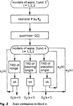
estimates of the state component in the block. The estimates of three state components are obtained sequentially, component-by-component, and in parallel by using the Viterbi algorithm since the quantisation levels of a state component at time k

+

1 depend upon the estimates of the other state components at time k. Fig. 2 shows a

replace Y byYd

55

quantiser Q{.}

k4

1

elevation angle O l ( k + l ) 0 2 ( k + l ) 0 3 ( k + l ) Fig. 2

VA: Viterbi algorithm; TRD: trellis diagram State estimation in block n

block diagram of the sequential state estimation of three state components (range, bearing angle, and elevation angle) in parallel in the nth block, where

ei(k)

a

{%dl

I

k): 1 = k - 1, k}

o J k + 1 ) P { 2 i ( l l k + 1 ) : ( n - 1 ) B < l < k + 1 and (n - l)B < k

-=

nB} Y {w(k), Zi(k), x,(O), x2(0), x3(0),

i l ( O ) , i 2 ( 0 ) , n3(0)1

{ w A ~ ) ,

ZiAk), x,q(O), x2q(O), x3q(O),

i i A O ) , i 2 A % i 3 A O ) )

5

where i = 1,2, 3. The estimates of a state component in a desired interval are the union of the estimates of the component in preselected blocks of the interval.

The performance of the proposed scheme is determined by the performances of the Viterbi algorithms used in parallel to estimate three state components in blocks. The performance of a Viterbi algorithm may not be exactly determined, but can be quantified by a Gallager- type ensemble upper bound [l, 8,9], since the evaluation of the exact error probability or error probability bound for choosing the correct path through the trellis diagram of a state component is complex. Such an ensemble upper bound is presented in Reference 1. However, one should note that ensemble bounds do not exactly determine the performance of the new approach since they are bounds averaged over ensembles [ 13.

4 Simulations

The range, bearing angle and elevation angle models which are given by eqns. 5-7 of Section 7.1, and many 1EE PROCEEDINGS, Vol. 136, Pt. F , No. 6, DECEMBER 1989

observation models containing white Gaussian interferences and observation noises were simulated for differ- ent parameters on an IBM 3081 K main-frame computer. The states of these models were estimated by the proposed estimation scheme. They cannot, in general, be estimated by the extended Kalman filter, owing to nonlinear interferences contained in the observation models; hence, the proposed scheme is superior to the extended Kalman filter.

In target tracking in the presence of interference, if a tracker were to be employed which used the extended Kalman filter and which was designed for target tracking in a clear environment (i.e. no interference), the state estimates would diverge from the actual state values. This has been demonstrated by estimating the states of the models of eqns. 5-7 with eqn. 2 by using the extended Kalman filter (EKF) assuming zero interference. For state estimation with the (extended) Kalman filter assuming zero interference, the approximate spherical models of the range, bearing angle and elevation angle which are presented in Reference 5 were used. The resulting estimates are said to be the EKF estimates of the states.

In state estimation with the proposed scheme, the dis- crete random variables given by Demirbas [l] were used to approximate the random variables in the state and observation models. These discrete random variables were assumed to be stationary. Two blocks with B = 4

were used for state estimation.

The simulation results of two example sets of observation models containing white Gaussian interferences and observation noises are presented in Figs. 3 and 4. Set 1 (Fig. 3) shows an example of the cases where only the state components are multiplied by nonlinear inter- ferences. Set 2 (Fig. 4) shows an example of the cases where both state components and observation noises are multiplied by nonlinear interferences. Figs. 3u-c present the actual values, EKF estimates, and the proposed estimation scheme estimates (SDSA) of the range, bearing angle, and elevation angle when the observation component models are given by

z2(k) = x2(k){ 1

+

0.2 sin [ 1 2 ( k ) ] }

+

u2(k) z , ( k ) = x,(k){l

+

0.5 sin [ Z , ( k ) ] }

+

o,(k)

z J ~ ) = x3(k){ 1

+

0.2 sin [ I , ( k ) ] }

+

4)

where the variances of the observation noises, the disturbance noises, the interferences, the components of the known deterministic pilot command vector, and the expected values of the interferences in the range, bearing angle, and elevation angle directions are (5.5 km2, 0.025 rad2, 0.025 rad2), (6.0 km2/s4, 2.5 km2/s4, 2.5 km2/

s4), (0.5, 0.3, 0.3), (1.5 kmz/s4, 0.06 km2/s4, 0.07 km2/s4), and (0.7, 0.4, 0.4), respectively. The variances, the derivatives, and the expected values of the initial range, bearing angle, and elevation angle are (5.0 km2, 0.02 rad2,

0.02 rad2), (2.0 km/s, 0.15 rad/s, 0.15 rad/s), and (55.0 km, 1.250 rad, 1.250 rad), respectively. The quantiser gate

sizes for the range, bearing angle and elevation angle are

0.01 km, 0.002 rad, 0.002 rad, respectively. The sampling

interval is 0.1 s. The viscous drag coefficient is 0.5 s-'. The initial range, bearing angle, elevation angle, interferences and disturbance noises were approximated by the random variables with three possible values [ 11.

Fig. 4 shows the actual values, EKF estimates and SDSA estimates of the range, bearing angle and elevation angle when the observation component models are given

(5)

1.6 3.0 4.8 6.4 8.0 1 C 521 I 1 I I 1 0 0 1.6 3.0 4.8 6.4 8.0 time, s a

S

_:

I

,

0.8 0 1.6 3.2 4.8 6.4 8.0 time, s b 2 0 . 8 8 0 1.6 3.2 4.8 6.4 8.0 time, s C Fig. 3

(c) elevation angle with set I observation component models

0 actual; A EKF; x SDSA

Actual and estimated values of (a) range, (b) bearing angle and

time, s a 3.0 time, s b - %

2

4 - 0 > 3 E .- c m 1.6 3.2 4.8 6.4 8.0, 0 time, s c Fig. 4

(c) elevation angle with set 2 observation component models

0 actual; A EKF; x SDSA

Actual and estimated values of (a) range, (b) bearing angle and

(6)

+

{exp C12(k)l)%(k) Set 2

1

Z 2 ( N = x , ( k ) { l + I 2 ( 4 sin CIZ(k)l)

Z 3 ( k ) = x3(k){l

+

I J k ) COS CI,(k)I)

+

(exP [13(k)l}h(k)

where the variances of the observation noises, the disturbance noises, the interferences, the components of the known deterministic pilot command vector, and the expected values of the interferences in the range, bearing angle, and elevation angle directions are (9.8 km2,

0.3 rad2, 0.3 rad2), (11.0 km2/s4, 1.9 km2/s4, 1.9 km2/s4),

(0.15, 0.2, 0.2), (3.3 km2/s4, 0.09 km2/s4, 0.09 km2/s4), and (0.33,0.2,0.2), respectively. The variances, the derivatives, and the expected values of the initial range, bearing angle, and elevation angle are (3.0 km2, 0.01 rad2, 0.01 rad2), (3.8 km/s, 0.02 rad/s, 0.02 rad/s), and (59.0 km,

0.35 rad, 0.28 rad), respectively. The rest of parameters are the same as in Set 1.

It should be noted that the observation models of Sets

1 and 2 are nonlinear functions of white Gaussian interferences. Hence, state estimation of the component models of eqns. 5-7 with these observation models cannot be done by using the extended Kalman filter, whereas the proposed scheme can be used for this estimation. The models of eqns. 5-7 and observation sets above are better approximated by the models of eqns. 3 and 4 for smaller gate sizes, greater block lengths, or greater numbers of possible values of the discrete random variables and vectors in eqns. 3 and 4. However, the imple- mentation complexity of the proposed scheme increases with these gate sizes, block lengths, or numbers. Thus, while preselecting these gate sizes, block lengths, and numbers a compromise has to be made between a desired estimation accuracy with available memory and the implementation complexity of the proposed scheme. Good state estimates can be obtained by the proposed scheme by choosing appropriate values for these gate sizes, block lengths and numbers. Simulation results showed that, when discrete random variables with three possible values were used in eqns. 3 and 4, good estimates of state components were obtained. In Figs. 3 and 4 the

SDSA estimates closely follow the actual component values, whereas the divergence of the Kalman estimates are caused by the zero interference assumption and linearisation errors of the models of eqns. 5-7.

5 Conclusions

A new suboptimum estimation scheme has been presented. This can be used to track a target in the presence of an arbitrary random interference, whereas estimation schemes based upon the extended Kalman filter may not. The implementation of the proposed scheme requires much more memory and computation than does the implementation of the extended Kalman filter. In state estimation with the proposed scheme the state (or motion) and observation models are not limited to models which are linear functions of the disturbance and observation noise, whereas in state estimation with the extended Kalman filter these models must be linear functions of the disturbance noise and observation noise. The observation model for each state component for the pro- I E E PROCEEDINGS, Vol. 136, Pt. F , N o . 6, DECEMBER 1989

posed scheme must be a function of this state component only. However, this model can be any function of interference. The only assumption made with regards to the initial state, disturbance noise, observation noise and interference is independency from time to time. The implementation of the proposed scheme requires a memory which increases exponentially with time in a block, even though it is independent of the number of blocks used. Hence, an approximate block size should be chosen for a satisfactory estimation accuracy with available memory.

6 References

1 DEMIRBAS, K.: ‘New smoothing algorithms for dynamic systems with or without interference’. The NATO AGARDOgraph advances in the techniques and technology of applications of nonlinear filters and Kalman filters, No. 256, AGARD, March 1982, pp. 19-1/66 2 DEMf RBAS, K. : ‘Maneuvering target tracking with hypothesis

testing’, IEEE Trans., 1987, AFS-23, (6), pp. 757-766

3 WHALEN, A.D.: ‘Detection of signals in noise’ (Academic Press, New York, 1971)

4 SAGE, A.P., and MELSA, J.L.: ‘Estimation theory with applications to communications and control’ (McGraw-Hill, New York, 197 1)

5 GHOLSON, N.H., and MOOSE, R.L.: ‘Maneuvering target track- ing using adaptive state estimation’, ZEEE Trans., 1977, AES-13, (3), pp. 31&317

6 MILLER, K.S., and LESKIW, D.M.: ‘Nonlinear estimation with radar observation’, IEEE Trans., 1982, AES18, (2), pp. 192-200 7 FORNEY, JR., G.D.: ‘Convolution codes 11. Maximum likelihood

decoding’, In$ & Control, 1974,25, pp. 222-266

8 GALLAGER, R.G.: ‘A simple derivation of the coding theorem and some applications’, IEEE Trans., 1965, IT-11, (l), pp. 3-18 9 VITERBI, A.J., and OMURA, J.K.: ‘Principles of digital communi-

cation and coding’ (New York, McGraw-Hill, 1979)

10 NAHL, N.E.: ‘Optimal recursive estimation with uncertain observa- tion’, IEEE Trans., 1969, IT-15, (4), pp. 457-642

11 MONZINGO, R.A.: ‘Disease optimal linear smoothing for systems with uncertain observation’, ZEEE Trans., 1975, IT-21, (3), pp. 271-275

7 Appendix

7.1 State component models

This Section states the models for the range, bearing angle and elevation angle of the location of a manoeuvring target. These models are derived in Reference 2. Let the components x,(k), x2(k) and x3(k) of the state vector x(k) represent the range, bearing angle and elevation angle of the target location at time k, respectively. The models for these components are given by

x,(k

+

1)

%CW,

x,(k), XAk), X3(k),

f(4,

441

= ( { X l ( k )

+

a 1 W d

+

azCu,(k)

+

W1(k)N2

+

{“1Xi(k)22(k) COS Cx3(k)I

+

a2CUz(k)

+

w2(k)l)2

+

{aiXi(k)23(k)

+

a2CUdk)

+

W3(k)I)2>1’2 ( 5 ) which is the range model,

x2(k

+

1) + f 2 C W , x 2 ( k ) , x,(k), X3(k),

f(4

441

(7) 267

(7)

which is the elevation angle model, where (1 - e-””? p At - 1

+

e-”*‘ E l - CL P Z a t -

In these equations p is the viscous drag coefficient; the overdot denotes the derivative with respect to time; At is the observation interval; w,(k), wZ(k), and w3(k) are the

components of a zero-mean white Gaussian disturbance noise vector w(k); and u,(k), u,(k), and uj(k) are the com-

ponents of a known deterministic pilot command vector u(k) affecting the target motion at time k in the range, bearing angle and elevation angle directions, respectively. time 0 time 1 time 2 time0 time1 time 2 time0

The nonlinear functions fl[.], fz[.] and f3[.] (defined

by eqns. 5-7) describe the components of the state vector at time k

+

1 in terms of the disturbance noise vector, pilot command vector and state vector at time

k.

It should be noted that these models are nonlinear functions of the state vector x(k) and disturbance noise vector

w(4.

7.2 Viterbi algorithm

This section describes the Viterbi algorithm which sys- tematically examines the metrics of all paths to find the path with the greatest metric through a trellis diagram, say from time zero to time L. Steps of the Viterbi algorithm are as follows :

Step k (k = 1, 2 , 3 , . . . , L): Consider each node at time k. Find the metrics of all the paths terminating at this node. Choose the path with the greatest metric (if more than one paths with the same greatest metric exist, then choose anyone of these at random), and discard the rest of the paths terminating at the node at time k. This process yields a new trellis diagram, which has only one path terminating at each node at time k. This new trellis diagram is called the trellis diagram at step k.

Final step (step L): Find the trellis diagram at step L.

Then find the path with the greatest metric through this trellis diagram (if there are more than one paths with the same greatest metric, then choose anyone of these at random). This path is the one having the greatest metric through the trellis diagram from time zero to time L.

As an example, consider the trellis diagram given in Fig. 5a. In this diagram, for convenience, the quantisation levels are denoted by integers. Let the integer sequence

u1a2a3, ..., a, and M [ a l a z u 3 , ..., aJ denote the path connecting the quantisation levels a,, u 2 ,

. .

. , a, and the metric of this path, respectively. At step 1, assume that

M[23] 2 M[13] and M[14] 2 MC241. This result in the

trellis diagram of Fig. 5b. At step 2, assume that

M[257] 2 MC1471 and MC2371. This result in the trellis

diagram of Fig. 5c. Finally assume that A411461 2 M[257]. Then the path 146 is the path with the greatest metric. time1 time 2

e 3 6e,,.

Fig. 5 Trellis diagrams

a Of state

b At stem 1

a b

268

C c At step 2