934
|
© 2018 International Society for Magnetic Resonance in Medicine wileyonlinelibrary.com/journal/mrm Magn Reson Med . 2019;81:934–946.F U L L PA P E R
bSSFP phase correction and its use in magnetic resonance
electrical properties tomography
Safa Ozdemir
|
Yusuf Ziya Ider
Department of Electrical and Electronics Engineering, Bilkent University, Ankara, Turkey Correspondence
Yusuf Ziya Ider, Department of Electrical and Electronics Engineering, Bilkent University, Ankara, Turkey. Email: [email protected] Funding information
This study was supported by TUBITAK 114E522 research grant. Experimental data were acquired using the facilities of UMRAM, Bilkent University, Ankara.
Purpose: Balanced steady‐state free precession (bSSFP) sequence is widely used
because of its high SNR and high speed. However, bSSFP images suffer from “band-ing artifact” caused by B0 inhomogeneity. In this article, we propose a method to
remove this artifact in bSSFP phase images and investigate the usage of the corrected phase images in phase‐based magnetic resonance electrical properties tomography (MREPT).
Theory and Methods: Two bSSFP phase images, obtained with different excitation
frequencies, are collaged to get rid of the regions containing banding artifacts. Phase of the collaged bSSFP image is the sum of the transceive phase of the RF system and an error term that depends on B0 and T2. By using B0 and T2 maps, this error is
elimi-nated from bSSFP phase images by using pixel‐wise corrections. Conductivity maps are obtained from the uncorrected and the corrected phase images using the phase‐ based cr‐MREPT method.
Results: Phantom and human experiment results of the proposed method are
illus-trated for both phase images and conductivity maps. It is shown that uncorrected phase images yield unacceptable conductivity images. When only B0 information is
used for phase correction conductivity, reconstructions are substantially improved, and yet T2 information is still needed to fully recover accurate and undistorted
con-ductivity images.
Conclusions: With the proposed technique, B0 sensitivity of the bSSFP phase
im-ages can be removed by using B0 and T2 maps. It is also shown that corrected bSSFP
phase images are of sufficient quality to be used in conductivity imaging.
K E Y W O R D S
banding artifact, bSSFP, conductivity, MREPT, phase‐based
1
|
INTRODUCTION
Impedance imaging aims at reconstructing conductivity, σ,
and permittivity, ϵ, of the tissues. Earlier methods of
imped-ance imaging are electrical impedimped-ance tomography (EIT)1,2
and magnetic induction tomography (MIT)3 that are used to induce currents in the object by using either surface electrodes (EIT) or external coils (MIT). However, these methods yield
images that have low spatial resolution in interior regions be-cause the measurements (i.e., surface potentials) are not very sensitive to electrical property perturbations relatively far from the surface. To overcome this weakness, magnetic res-onance electrical impedance tomography (MREIT) has been introduced.4-9 In MREIT, current is induced by using surface
electrodes in the frequency range of 10 Hz–10 kHz and the resulting magnetic field is measured by MRI to reconstruct
(γ = σ + iωϵ) can be derived as follows :
With the assumption of locally constant electrical proper-ties, known as “local homogeneity assumption” (LHA), the gradient term (
∇γ
γ ×(∇ × B + 1
)) is eliminated and admittivity
becomes:
Although Equation (2) is widely used for obtaining elec-trical property images, this method suffers greatly from boundary artifacts, because of the elimination of the gradient term in Equation (1). To solve this issue, as also reviewed in Liu et al.13 and Katscher and van der Berg,14 several
ap-proaches are followed.15-17 The approach of Hafalir et al.15 introduces the convection–reaction partial differential equa-tion (PDE)‐based method (cr‐MREPT), which is, in fact, the solution of Equation (1) using numerical techniques. The approach of Liu et al.16 uses similar formulation in their method called gradient‐based electrical properties tomogra-phy (gEPT). In this method, with the knowledge of B+1 that
is obtained by using a multi‐channel transceiver RF coil, gra-dient of the electrical properties is obtained. Through spatial integration starting from a seed‐point, both conductivity and permittivity are obtained. Contrast source inversion‐based EPT (CSI‐EPT) views the object as a scatterer placed in the field generated by the RF coil.17 EPs are updated until the measured RF field matches closely the field calculated by the solution of the integral–equation‐based forward problem expressing the magnetic field as a function of the EPs.
For the aforementioned methods, both the phase and magnitude of B+1 are to be measured. Although there are
well‐established techniques to obtain the magnitude of
B+1,18-20 phase of B+1 cannot be measured directly in MRI. For
birdcage‐like quadrature volume coil configurations, trans-mit phase is roughly taken as half of the transceive phase.
to find conductivity where is the transceive phase (if trans-mit phase is used, the factor 2 in the denominator is otrans-mit- omit-ted).21 Although this “standard” phase‐based formulation is
free from TPA and does not require B+1 mapping, it assumes
low B+1 magnitude gradients, in addition to using LHA. While
LHA causes well‐known tissue‐boundary artifacts in the conductivity images as mentioned before, assuming low B+1
magnitude gradient causes errors in the reconstructed conduc-tivity values (up to 10% for 3 T systems)21 especially toward
the boundary of the imaged object.24 Recently, a phase‐based
EPT method that does not require LHA, but still assumes low B+1 gradients, was introduced by Gurler and Ider.25 With
this approach, called “phase‐based cr‐MREPT technique,” boundary artifacts in the conductivity images are significantly reduced. (Note that the methods mentioned in the previous paragraph in reference to Hafalir et al.,15 Liu et al.,16 and
Balidemaj et al.17 aim at reducing boundary artifacts in full B+1 ‐based methods that use both the phase and the magnitude
of B+1. Gurler’s approach, on the other hand, is similar in
con-cept to Hafalir et al.15 but uses only the phase of B+ 1).
To reconstruct conductivity using the phase‐based ap-proach, any MR sequence that provides B+1 phase can be
used. Commonly used sequences are spin‐echo,23 gradient
echo,26 UTE/ZTE,27,28 and balanced steady‐state free
preces-sion (bSSFP).29 Spin‐echo suffers from eddy current effects
and lengthy acquisition time. Gradient echo suffers from off‐ resonance effect, which needs to be corrected by additional
B0 mapping. In addition to this, eddy currents and
acquisi-tion time are still problematic. UTE/ZTE, despite being fast sequences, suffer from streaking artifacts that deteriorate the phase images, and such artifacts can be amplified through Laplacian operation and distort the final conductivity image. bSSFP is favorable to obtain phase images because it has high speed, high SNR, motion insensitivity, and automatic eddy current compensation because of balanced gradients.14,29 On
the other hand, it suffers greatly from B0 inhomogeneity and
the concomitant “banding artifact.” In regions of banding ar-tifact, MR signal reduces significantly and also phase errors occur. As shown later, for low T2 values, these phase errors
are even more prominent. (1) −∇2B+ 1= ∇γ γ ×(∇ × B + 1) − iωμ0γB + 1. (2) γ = ∇ 2B+ 1 iωμ0B+1.
The purpose of this study is to correct the phase errors in images obtained by the bSSFP sequence to make it an accept-able sequence for phase‐based MREPT. In general, a method that makes use of B0 and T2 maps, and 2 bSSFP runs with an
excitation frequency difference of (2TR)−1 is developed to
correct the phase distribution obtained by bSSFP. Following the sections that explain the theory and the rational of the method, phantom image reconstructions and head data re-sults using phase‐based cr‐MREPT technique are presented.
2
|
THEORY
2.1
|
Dependence of bSSFP phase on ΔB
0and T
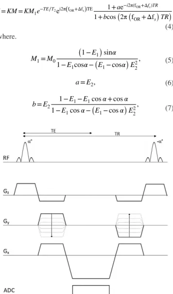
2bSSFP sequence using alternating RF pulses is shown in Figure 1. In bSSFP imaging, the complex image value at an arbitrary pixel in the slice of interest, can be expressed as30,31:
where.
T1 and T2 represent longitudinal and transversal relaxation
times, TE and TR are echo time and repetition time, α is flip
angle, M0 is equilibrium magnetization, fOR is off‐resonance
frequency because of ΔB0, Δfs is the frequency shift in the
excitation frequency as controlled by the user, and K is the
complex valued factor the phase of which is the transceive phase of the RF system (sum of transmit phase and receive phase). Although magnitude of S is dependent on many
pa-rameters, phase of it, which is the measured bSSFP phase, is relatively simple and can be expressed as:
where
In Equation (10), ∠(K) is what we are interested in and ∠(M) can be viewed as a phase error term. In the
expres-sion for the phase error term, the independent variables are T2 (through E2), the off‐resonance frequency fOR, TE, TR,
and the excitation frequency shift Δfs. Among these, TE, TR,
and the excitation frequency shift are determined by the user. Therefore, by making use of methods for determining the off‐ resonance frequency and T2 values for each pixel, we can
ob-tain the correct value of transceive phase for each pixel using Equations (10) and (11). Note that, if E2= 1 (infinite T2), then ∠(M) is either 0 or π (see Appendix).
Figure 2 demonstrates magnitude and phase of M with
re-spect to off‐resonance as obtained from Equation (4). Figure 2A and B are for a large T2 (T2 = 1000 ms), and the graphs
are given for two cases: (1) frequency shift Δfs equals 0 (blue
lines), and (2) frequency shift Δfs equals 1/2TR (red lines).
Concentrating on the magnitude graph for 0 frequency shift (the blue line in Figure 2A), we see that, for 0 off‐resonance, the magnitude of M is maximum, and as off‐resonance
in-creases, the magnitude begins to decrease and the decrease becomes substantial as the off‐resonance approaches (2TR)−1
(banding artifact). The magnitude increases again with further increase in off‐resonance, and this off‐resonance dependent behavior is periodic with a period of (TR)−1. The
off‐resonance frequency range is divided into 2 parts, called the “pass‐band” and the “stop‐band” regions.32 The pass‐
band region corresponds to a region in which magnitude is high, and stop‐band region corresponds to the region where magnitude is low. These 2 regions are non‐intersecting and their union covers the whole range. The exact definitions of these regions depend on the application and the purpose of (4) S= KM = KM1e−TE∕T2ei2π(fOR+Δfs)TE 1+ ae−i2π(fOR+Δfs)TR 1+ bcos(2π (fOR+ Δfs) TR) , (5) M1= M0 (1 − E1) sin𝛼 1− E1cos𝛼−(E1− cos𝛼) E2 2 , (6) a= E2, (7) b= E2 1− E1− E1cos 𝛼+ cos 𝛼 1− E1cos 𝛼−(E1− cos 𝛼) E 2 2 , (8) E1= e− TR T1, (9) E2= e− TR T2. (10) ∠(S) = ∠(K) + ∠(M), (11) Δ(M) = 2π(fOR+ Δfs) TE + Δ ( 1+ E2e−i2π(fOR+Δfs)TR ) .
FIGURE 1 Pulse sequence diagram for the RF alternating balanced steady‐state free precession (bSSFP) sequence used in this study
the study.32 In our case, we have decided to determine them
as follows: in the base period [
−2TR1 < f < 2TR1 ] , pass‐band is defined as [ − 1 4TR < f < 1 4TR ]
, and the stop‐band is the rest
of the period. The boundaries of these regions are shown in Figure 2 for the base period and also for the adjacent periods. For the graph for which excitation frequency shift is equal to (2TR)–1 (the red lines in Figure 2A and B), we observe that
the magnitude and phase graphs shift exactly by an amount
of (2TR)–1 with respect to the blue lines. Therefore, using the
same definition of pass‐band and stop‐band regions for these red graphs reveal regions such that the pass‐band region of the blue graphs corresponds exactly to the stop‐band region of the red graph and vice versa. The reason why stop‐band and pass‐band regions are selected as explained above will be apparent later.
When we look at the phase graphs, we observe that in the pass‐band regions, phases are almost constant; however, in the
FIGURE 2 (A) Magnitude and (B) phase of the steady‐state magnetizations as a function of off‐resonance for T2 = 1000 ms, and (C and D)
T2 = 40 ms are shown. Blue lines correspond to the magnetizations that are obtained with bSSFP sequence using alternating RF pulse, whereas
red lines correspond to the same sequence but excitation frequency difference of 50 Hz. Simulation parameters are: T1 = 6000 ms, TE = 5 ms,
middle of stop‐band regions, a jump of π radians is observed. This jump corresponds to the phase jump in the banding arti-fact of bSSFP images. When the blue phase lines and the red phase lines are compared, it is observed that the difference of the phase in the pass‐band region of the red line and the phase in the pass‐band region of the blue line may be either 0 or π radians except for a very narrow transition region. Please note that these observations are made for the case of large T2 (i.e.,
T2= 1000 ms). For infinite T2, the aforementioned narrow
transition region would be infinitesimally small.
Figure 2C and D present the graphs for a small T2 (T2
= 40 ms). One can observe that the magnitude plots do not display a constant plateau behavior, even in the pass‐band re-gion, and begin to decrease at lower off‐resonance frequen-cies. Similarly, the phase graphs also do not display almost constant behavior in the pass‐band regions but display a variation dependent on both ΔB0 and T2. For example, for
small ΔB0, dependence on ΔB0 is almost linear, and the slope
is equal to 1 2−
E2
1+E2. We called this variation of phase in the pass‐band regions “non‐constant plateau effect.”
3
|
METHODS
3.1
|
Method for correcting phase errors
because of
𝚫B
0and T
2The method comprises the acquisition of 2 bSSFP images, 1
B0 map, and 1 T2 map. Using the information contained in the
B0 map, a bSSFP image is segmented into 2 segments (set of
pixels). One segment corresponds to pixels for which ΔB0 lies
in the pass‐band region of the magnetization versus off‐reso-nance curves shown in Figure 2, and the other segment con-tains pixels at which ΔB0 corresponds to the stop‐band region.
The 2 bSSFP images are obtained with different excitation frequencies. Difference between the 2 excitation frequencies is selected as (2TR)−1, because periodicity of regions (pass‐band
and stop‐band) is (TR)−1 (how these excitation frequencies are
determined is explained in Sequence Protocols section). In this way, we have complementary images such that, if 1 pixel lies in the pass‐band segment in 1 bSSFP image, it lies in the stop‐band segment in the other bSSFP image. The boundar-ies between the pass‐band and stop‐band segments are called “the band transition boundaries.” A third image is generated by combining the pass‐band segments extracted from each of the bSSFP images. In other words, this “collaged” image is formed by making use of the banding artifact‐free segments of each of the 2 bSSFP images. However, the phase of the collaged image still has contributions from the phase error term explained in Equations (10) and (11). Phase error is cal-culated for any pixel by ∠(M) as given in Equation (11), using
the T2 and ΔB0 values of that pixel. Calculated phase error
is subtracted from the collaged image to obtain ΔB0 and T2
corrected phase maps. If T2 map is not available, one can take
E2= 1 and make the phase correction accordingly, in which
case the corrected phase image is called “type‐I corrected phase image.” If both ΔB0 and T2 maps are available, E2 is
assigned to its correct value for each pixel and the corrected phase image is called “type‐II corrected phase image.”
3.2
|
Phase based cr‐MREPT
Instead of the standard phase‐based MREPT method ex-pressed by Equation (3), the approach by Gurler and Ider is used to obtain conductivity from the phase maps.25 This
method is based on the convection–reaction PDE for resistiv-ity, ρ, as given below:
where ρ = 1∕σ, and ϕ is the transceive phase. The
convec-tion term (∇φ × ∇ρ) helps to combat the boundary artifact problem. For regularization purposes, and also to minimize spurious oscillations occurring along the internal tissue boundaries, an artificial diffusion term is added to this equa-tion as follows25,33:
where c is the constant diffusion coefficient. Because the dif-fusion term also has a low‐pass filter effect, higher values of
c result in loss of resolution, whereas lower values of c are not
sufficient to eliminate oscillations. To find optimum value of
c, different values from 0.001 to 0.05 are tried, and 0.015 is
selected by visual inspection.
This method can be applied to any 3D region of interest (ROI). Given the 3D phase map, a 2D ROI is selected visu-ally from any z‐slice and the ROI is extended to a 3D vol-ume ROI by specifying the number of slices to be included above and below the initial slice. For z‐independent ρ
dis-tributions, such as in the experimental phantom explained below, the PDE can be reduced to its 2D form and solved in a 2D ROI in the slice of interest.25 The pixels lying on
the boundary of the ROI are used to specify a Dirichlet boundary condition of ρ = 0.5 S/m. It is known that the use
of artificial diffusion, as shown in Equation (13), makes the solution not so sensitive to the boundary condition for voxels more than few layers inside the ROI. This issue, the numerical solution method, and the various assump-tions inherent in the phase‐based cr‐MREPT method are explained in Gurler and Ider.25
3.3
|
Phantom setup
A cylindrical, z‐independent experimental phantom with di-ameter of 20 cm and height of 25 cm was constructed. For background region, agar‐saline gel (20 g/L agar, 2 g/L NaCl, (12)
(∇φ ⋅ ∇ρ) +(∇2φ)𝜌− 2𝜔𝜇0= 0,
(13)
0.2 g/L CuSO4) was used, and for anomalies, longitudinal
holes were drilled and filled with saline solution (6 g/L NaCl, 0.2 g/L CuSO4). The conductivity values for background and
the anomaly regions are expected to be 0.5 and 1 S/m, re-spectively.15 Anomaly regions have diameters of 0.5, 1.5,
and 2.5 cm, and they are visible in the MR magnitude image of the middle slice of the phantom in Figure 3A.
3.4
|
In vivo human experiment
MRI scans were performed on a healthy, 25‐year‐old male volunteer after obtaining written informed consent in line with the approval of the Institutional Review Board of Bilkent University.
3.5
|
Sequence protocols
For obtaining the B+1 phase, 2 bSSFP sequences are used
(Figure 1). The sequence parameters in the phantom ex-periment were: TE/TR = 5/10 ms, FOV = 225 mm, voxel size = 1.76 × 1.76 × 1.5 mm, FA = 40°, NEX (number
of averages) = 32, number of slices = 20, and duration for each scan = 5:29 min/s. In the human experiment, the pa-rameters were: TE/TR = 5/10 ms, FOV = 225 mm, voxel size = 1.76× 1.76 × 1.5 mm, FA = 40°, NEX = 8, number
of slices = 60, and duration for each scan = 10:14 min/s. For the first bSSFP sequence, the RF excitation frequency, f1, is
determined by the MRI system itself. For the second bSSFP sequence, we have used an RF frequency, f2, which is equal
to f1+ 50 Hz. Because TR is equal to 10 ms, the frequency
shift is chosen as (2TR)−1= 50 Hz.
B0 map is the obtained by using the double echo method
that involves 2 gradient echo images with different TEs.34
The sequence parameters in the phantom experiment were: TE = 10 or 15 ms, TR = 3500 ms, FOV = 225 mm, voxel size = 1.76× 1.76 × 1.5 mm, FA = 60°, number
of slices = 20, and duration for each scan = 7/33 min/s. In the human experiment the parameters were: TE = 10 or 15 ms, TR = 3500 ms, FOV = 225 mm, voxel size =
1.76× 1.76 × 1.5 mm, FA = 60°, number of slices = 60,
and duration for each scan = 7/33 min/s. T2 map is obtained
via a series of single echo spin‐echo sequences with differ-ent TEs by using the expondiffer-ential T2 fitting method whose
result is accepted as the ground truth for many investiga-tors.35,36 The sequence parameters in the phantom experiment
were: TE = 13, 30, 50, 75, 100, or 150 ms, TR = 3500 ms, FOV = 225 mm, voxel size = 1.76× 1.76 × 1.5 mm,
num-ber of slices = 20, and duration for each scan = 7/33 min/s. In the human experiment, the parameters were: TE = 13, 40, 75, or 100 ms, TR = 6500 ms, FOV = 225 mm, voxel size =
1.76× 1.76 × 1.5 mm, number of slices = 60, and duration
for each scan = 14/00 min/s. Note that, the gradient echo and the spin echo sequences that we have mentioned above are all multi‐slice sequences in which data are collected from all slices within 1 TR, and therefore the total duration of such multi‐slice scans is dependent on TR and not dependent on the number of slices. Both of the B0 and T2 maps are obtained
by using the RF excitation frequency equal to f1. Experiments
were conducted on 3 T Siemens Tim Trio MR scanner (Siemens, Erlangen, Germany) using a quadrature body coil.
For the human experiments, a Gaussian filter with a kernel size of 5 × 5 × 5 voxels and a SD of 1.06 for each direction
experiment, (A and B) magnitude and (C and D) phase images obtained by the 2 bSSFP sequences. In all images banding artifacts shown by white arrows [Colour figure can be viewed at wileyonlinelibrary. com]
was applied to the transceive phase data. No low‐pass filter is applied to the data obtained in the phantom experiment.
4
|
RESULTS
Magnitude and phase of the phantom images obtained by the 2 bSSFP sequences are shown in Figure 3A–D. Figure 3A and C correspond to the RF alternating bSSFP sequence ap-plied by using the RF frequency that is determined by the MRI system, f1. Figure 3B and D correspond to the RF
al-ternating bSSFP sequence applied using the shifted RF ex-citation frequency, f2= f1+ 50 Hz. Banding artifacts in the
magnitude images, characterized by loss of signal, are shown by white arrows (Figure 3A and B). It is observed that, as expected, banding artifacts lie in the iso‐ B0 lines in both
im-ages (refer to the B0 map in Figure 4B). In the phase maps, as
shown in Figure 3C and D, a phase shift of π, radians is ob-served in the banding artifact region. This shift is not phase‐ wrapping, because it occurs along several pixels as opposed to phase‐wrapping that occurs in a single pixel transition by an amount of 2π.
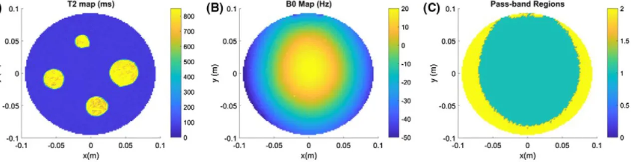
T2 and B0 maps for the phantom are shown in Figure 4A
and B. It is found that T2 values are 70 ms and 850 ms, on
average, for the background and anomaly regions, respec-tively. B0 map demonstrates that there are deviations from
central frequency, from −70 Hz to 30 Hz, indicating the ex-tent of B0 inhomogeneity. The pass‐band segments, which are
determined by using the B0 map, are shown in Figure 4C.
Cyan region corresponds to pixels that are away from band-ing regions in the first image and the yellow region corre-sponds to pixels that are away from banding regions in the second image. Putting it differently, cyan region corresponds to pixels that fall in the pass‐band segment of the first bSSFP experiment and yellow region corresponds to the pass‐band segment of the second bSSFP experiment.
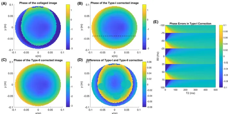
The phase of the collaged image, type‐I corrected phase image, and type‐II corrected phase image are shown in Figure 5A–C. Note that the phase jumps (for an amount of π) that are observed in the collaged image are corrected in the type‐I
corrected phase image as expected. Moreover, phase errors because of finite T2 values (E2 < 1, non‐constant plateau
effect) are also corrected for in the type‐II corrected phase image. To appreciate the extent of the correction based on T2
values, Figure 5D shows the difference of type‐II corrected phase image and type‐I corrected phase image. The range of the difference image is approximately ±0.06 radians (±3.5°). Phase differences between type‐I and type‐II corrections are largest near the band transition boundaries and also are dis-continuous across them. In the error map (Figure 5D), it is found that the phase error is small in the anomalies, and this is because of the fact that they have large T2 values (Figure
4A). Although the phase errors between type‐I and type‐II corrected images may be considered to be small for many applications, it will be shown below that use of type‐II cor-rection is essential, especially when conductivity reconstruc-tions are considered.
Figure 5E displays the expected (theoretical) phase differ-ences between type‐I and type‐II corrections as a function of T2 and ΔB0 as calculated by using Equations (10) and (11).
A phase difference does not occur if ΔB0 is 0 or a multiple
of 1/2TR (as also shown in Figure 2). It is also observed that phase differences between type‐I and type‐II corrections are largest near the boundaries between pass‐band and stop‐band regions and are also discontinuous across them. The reason why the error is largest near the boundaries between pass‐ band and stop‐band regions is that at these boundaries, ΔB0
corresponds to 1 4TR+
n
2TR where n is an integer, and these are
the off‐resonance frequencies at which T2 has maximal
ef-fect. Discontinuity of the error occurs because of the fact that T2 contribution to phase error, ∠(M), changes sign across the
boundary. With similar reasoning, discontinuity of the error in Figure 5D is because of the fact that pixels on either sides of the phase transition boundary are taken from different bSSFP images, and therefore T2 contributions to phase error, ∠(M), has opposite polarities across the boundary.
Conductivity maps that are obtained from uncorrected (original) bSSFP phase images using the phase‐based cr‐ MREPT technique are shown in Figure 6A and B. Severe conductivity artifacts occur in the banding artifact regions
FIGURE 4 For the phantom experiment, (A) T2 map, (B) B0 map, and (C) the pass‐band segments that are determined based on the B0 map
in both figures, even in regions where banding artifact is not fully onset. When the type‐I corrected phase image is used for conductivity reconstruction, significant improve-ment in conductivity image is obtained as shown in Figure 6C. However, in this case, there is still distortion in the con-ductivity reconstruction along the band transition boundary. These are caused by the errors in type‐I corrected images
because of the fact that T2‐based corrections are still not
per-formed, which are most prominent along and near the band transition boundaries (the ring artifact shown in Figure 6C). Although phase errors in type‐I are small, they still distort the conductivity image because their effects are amplified by Laplacian operation. Nonetheless, when the type‐II cor-rected phase image is used to reconstruct the conductivity,
FIGURE 5 For the phantom experiment, (A) phase of the collaged image, (B) phase of the type‐I corrected image, (C) phase of the type‐II corrected image, (D) difference between type‐I and type‐II corrected phase images, and (E) theoretical difference between type‐I and type‐II corrected phases as a function of ΔB0 and T2. The dotted line in (B) indicates the position of the profile plots shown in Figure 7. The unit of phase
in all images is radians [Colour figure can be viewed at wileyonlinelibrary.com]
FIGURE 6 For the phantom experiment, (A) conductivity map obtained from the phase image of the first bSSFP, (B) conductivity map obtained from the phase image of the second bSSFP, (C) conductivity map obtained from type‐I corrected image, and (D) conductivity map obtained from type‐II corrected image. The ring artifact shown in (C) by an arrow is because of the phase ripple observed along the band transition boundary as shown in Figure 7 [Colour figure can be viewed at wileyonlinelibrary.com]
FIGURE 7 For the phantom experiment, (A) phase of the type‐I corrected image drawn as 3D surface plot, (B) phase of the type‐II corrected image drawn as 3D surface plot, (C) phase profile of the type‐I corrected image, (D) phase profile of the type‐II corrected image, (E) conductivity profile of the type‐I corrected image, and (F) conductivity profile of the type‐II corrected image. The profiles are drawn along the line depicted in Figure 5B [Colour figure can be viewed at wileyonlinelibrary.com]
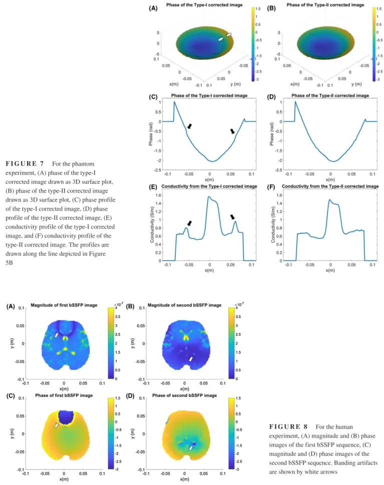
FIGURE 8 For the human experiment, (A) magnitude and (B) phase images of the first bSSFP sequence, (C) magnitude and (D) phase images of the second bSSFP sequence. Banding artifacts are shown by white arrows [Colour figure can be viewed at wileyonlinelibrary.com]
all artifacts are eliminated and a clean conductivity map is obtained (Figure 6D).
Figure 7A and B represent the type‐I and type‐II corrected phase images drawn as 3D surface plot. Small phase devia-tions near the band transition boundaries in type‐I corrected phase images are visible in Figure 7A and are shown by white arrows. Along the line that is depicted in Figure 5B, profiles for phase (Figure 7C and D) and conductivity (Figure 7E and F) for both type‐I and type‐II corrections are shown. Both the small phase deviations and the conductivity ripples cor-responding to the band transition boundaries are shown by black arrows (Figure 7C and E). Clearly, when type‐II cor-rected phase images are used, ripples in the conductivity er-rors are significantly reduced.
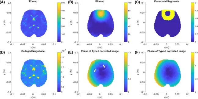
Human experiment results are shown in Figures 8–10. Figure 8 demonstrates the magnitude and phase of both bSSFP runs for a middle axial slice. Banding artifacts are shown by white arrows. T2 map, B0 map and pass‐band
segments, for the same slice, are shown in Figure 9A–C. Collaged magnitude is shown in Figure 9D. Type‐I and type‐ II corrected phase images are shown in Figure 9E and F. Although type‐I corrected phase image suffers from the small deviations and jumps because of non‐constant plateau effect (shown by white arrows), those errors are eliminated in the type‐II corrected phase image. 3D version of phase‐based cr‐ MREPT is used to obtain conductivity maps for 10 slices, and 2 different slices are shown in Figure 10. Because of band-ing artifact, there are severe distortions on conductivity maps
FIGURE 10 For the human experiment, reconstructed conductivities for 2 different slices of the brain for the human experiment. For the first slice, (A) conductivity map obtained from the first bSSFP phase image, (B) conductivity map obtained from the second bSSFP phase image, (C) conductivity map obtained from type‐I corrected phase image, (D) conductivity map obtained from type‐II corrected phase image, and (E) collaged magnitude image. (F–J) Corresponding images for the second slice. Although (A), (B), (F), and (G) suffer from banding artifact, (C) and (H) suffer from non‐constant plateau effect, (D) and (I) are free from such disturbances [Colour figure can be viewed at wileyonlinelibrary.com]
FIGURE 9 For the human experiment, (A) T2 map, (B) B0 map, (C) the images of the pass‐band segments that are determined based on the
B0 map, (D) collaged magnitude, (E) phase of the type‐I corrected image, and (F) phase of the type‐II corrected image. Small phase ripples at the
obtained from both bSSFP runs (Figure 10A, B, F, and G), and the effect of the non‐constant plateau is seen in Figure 10C and H, but conductivity images that are obtained from type‐II corrected phase (Figure 10D and I) do not include such distortions. Collaged bSSFP magnitudes for the 2 slices are also shown (Figure 10E and J) for comparison with the reconstructed conductivity images.
5
|
DISCUSSION AND
CONCLUSIONS
It has been argued that bSSFP is the most favorable phase‐ measuring method for MREPT because of its speed, motion insensitivity, automatic eddy current compensation, and high SNR.14,29 However, bSSFP phase is susceptible to
off‐reso-nance and T2 effects, and it is vulnerable especially in
cer-tain regions where banding artifact occurs. In this study, we have addressed this problem and have developed a method for obtaining correct RF phase throughout the object. It has also been shown that the correction method provides phase distributions that have sufficient quality for obtaining con-ductivity images.
We have demonstrated the use of our proposed bSSFP phase correction method in experiments performed in a 3 T scanner. The method proposed in this work is not dependent on the static magnetic field strength, but because, to our knowledge, high field systems have higher B0
inhomogene-ity, the use of the proposed method is even more indicated for high field systems.
The method that we have developed requires the acqui-sition of T2 and B0 maps as well as 2 bSSFP runs. In this
article, the T2 and B0 mapping techniques that we have used
take 45 min and 15 min, respectively, for the phantom ex-periment. In this study, we have preferred to use a reliable T2 mapping technique that is considered to be a golden
truth by many investigators,35,36 although there are faster
methods that may provide considerable reduction in the acquisition time. For example, a method based on multi‐ spin‐echo sequence is proposed in Ben‐Eliezer et al.,35 and
an involved compensation technique for the interfering stimulated echoes is used. Another method36 using 1 single
scan based on a triple echo steady‐state (TESS) sequence makes use of modeling the relation between the echoes and an iterative numerical solution for obtaining the T2 map.
MIRACLE37 is similar to TESS and merges TESS with a
balanced acquisition scheme for motion‐insensitive rapid configuration relaxometry. All these methods can be used to decrease T2 mapping time to 5–10 min. However, they
need to be carefully optimized for SNR and artifacts so that they are acceptable for MREPT. Other approaches that are based on estimating T1, T2, ΔB0, and potentially also
RF phase simultaneously from a model of the bSSFP data,
such as LORE31 and PLANET,38 can also be implemented
for obtaining the RF phase directly and within 5–10 min. Although these methods are implemented in Björk et al.31
and Shcherbakova et al.,38 results for RF phase are not
explicitly presented. Therefore, these methods need to be assessed for their performance with respect to RF phase and its use in MREPT. By introducing the aforementioned methods, scanning time might be reduced significantly, and therefore bSSFP may still maintain its comparative ad-vantages for obtaining conductivity images.
Conductivity reconstructions obtained for the experi-mental phantom have well‐defined internal boundaries and reasonably accurate conductivity values. Conductivity re-constructions of the in vivo human brain correlate with the bSSFP magnitude images that roughly correspond to the an-atomical structures. However, there are several approaches by which they can be improved. As for any multi‐scan‐based method, our proposed method would also be affected from the patient motion between scans. Although algorithms can be devised for correcting motion errors, we think one should be cautious in using them because they may result in jumps and distortions in conductivity reconstructions because of the Laplacian operation involved. Rather, by taking precau-tions against motion and by using faster data acquisition techniques, which are discussed above, conductivity errors caused by motion might be reduced. There may be phase off-set between scans, for example, if the excitation frequency for each scan is not set accurately. We have paid attention to scanner adjustments, and we have not encountered phase offsets while working with Siemens 3 T Tim Trio scanner. In addition, several pre‐ and post‐processing techniques may also be used for further improvement: better estimation of the Laplacian of the phase,28 use of proper combination of
multi‐channel data,39 using adaptive regularization,40 and
increasing the number of acquisitions for signal averaging are some of the possibilities. In our experiments, to obtain banding artifact with even smaller ΔB0 values, and therefore
be able to demonstrate the effectiveness of our algorithms, high values for TE/TR pair are used (5/10 ms). Using lower TE values (e.g. TE/TR = 2.5/5 ms) would increase SNR and would also reduce the acquisition time. As mentioned before, using phase‐based formulation rather than complex
B+1 ‐based formulation generates additional bias in the whole
conductivity image, especially toward the boundary of the imaged object.24 Therefore, the phase correction method
pro-posed in this study may also be used in complex B+1 ‐based
MREPT techniques.
In this article, we have used different excitation frequen-cies—the difference being equal to (2TR)−1 —for the 2
bSSFP sequence applications. However, instead of shifting the excitation frequency, one can also use RF phase cycling. In such a case, the formula for the complex image value, at an arbitrary pixel in the slice of interest becomes:
this π/2 offset.
It has been argued in the Methods section that by mak-ing use of methods for determinmak-ing the off‐resonance and T2 values for each pixel, one can obtain the correct value
of transceive phase for each pixel using Equations (10) and (11). This would even be possible with only 1 bSSFP run therefore avoiding the additional scan time of the sec-ond run. However, there is a fundamental drawback of Equations (10) and (11) for fOR values close to the
bound-aries between pass‐band and stop‐band regions. In these boundary regions, fOR dependence of phase is very steep,
and therefore even a small error in the measured fOR value
would result in an overly erroneous phase value. To avoid these ill‐conditioned regions of the magnetization versus off‐resonance graphs, we have chosen to use 2 bSSFP runs and use the pass‐band regions of either of them.
REFERENCES
1. Barber C, Brown B, Freeston I. Imaging spatial distributions of resistivity using applied potential tomography. Electron Lett. 1983;19:933.
2. McEwan A, Cusick G, Holder D. A review of errors in multi‐fre-quency EIT instrumentation. Physiol Meas. 2007;28:S197‐S215. 3. Griffiths H. Magnetic induction tomography. Meas Sci Technol.
2001;12:1126‐1131.
4. Woo EJ, Lee SY, Mun CW. Impedance tomography using internal current density distribution measured by nuclear magnetic res-onance. In: Proceedings of SPIE 2299, Mathematical Methods in Medical Imaging III; 1994; San Diego, CA, pp. 377–385. 5. Ider YZ, Birgul O. Use of the magnetic field generated by the
internal distribution of injected currents for electrical impedance tomography (MR‐EIT). Elektrik. 1998;6:215‐225.
6. Seo JK, Yoon JR, Woo EJ, Kwon O. Reconstruction of con-ductivity and current density images using only one compo-nent of magnetic field measurements. IEEE Trans Biomed Eng. 2003;97:1121‐1124.
7. Ider YZ, Onart S. Algebraic reconstruction for 3D magnetic reso-nance‐electrical impedance tomography (MREIT) using one com-ponent of magnetic flux density. Physiol Meas. 2004;25:281‐294.
13. Liu J, Wang Y, Katscher U, He B. Electrical properties tomog-raphy based on B1 maps in MRI: principles, applications, and challenges. IEEE Trans Biomed Eng. 2017;64:2515‐2530. 14. Katscher U, van den Berg C. Electric properties tomography:
biochemical, physical and technical background, evaluation and clinical applications. NMR Biomed. 2017;30:e3729.
15. Hafalir F, Oran O, Gurler N, Ider Y. Convection‐reaction equation based magnetic resonance electrical properties tomography (cr‐ MREPT). IEEE Trans Med Imaging. 2014;33:777‐793.
16. Liu J, Zhang X, Schmitter S, Van de Moortele P, He B. Gradient‐ based electrical properties tomography (gEPT): a robust method for mapping electrical properties of biological tissues in vivo using magnetic resonance imaging. Magn Reson Med. 2014;74:634‐646.
17. Balidemaj E, van den Berg C, Trinks J, et al. CSI‐EPT: a contrast source inversion approach for improved MRI‐based electric prop-erties tomography. IEEE Trans Med Imaging. 2015;34:1788‐1796. 18. Stollberger R, Wach P. Imaging of the active B1 field in vivo.
Magn Reson Med. 1996;35:246‐251.
19. Yarnykh V. Actual flip‐angle imaging in the pulsed steady state: a method for rapid three‐dimensional mapping of the transmitted radiofrequency field. Magn Reson Med. 2006;57:192‐200. 20. Sacolick L, Wiesinger F, Hancu I, Vogel M. B1 mapping by
Bloch‐Siegert shift. Magn Reson Med. 2010;63:1315‐1322. 21. Katscher U, Kim D, Seo J. Recent progress and future challenges
in MR electric properties tomography. Comput Math Methods
Med. 2013;2013:1‐11.
22. van Lier A, Brunner D, Pruessmann K, et al. B1+ Phase mapping at 7 T and its application for in vivo electrical conductivity map-ping. Magn Reson Med. 2011;67:552‐561.
23. Voigt T, Katscher U, Doessel O. Quantitative conductivity and permittivity imaging of the human brain using electric properties tomography. Magn Reson Med. 2011;66:456‐466.
24. van Lier A, Raaijmakers A, Voigt T, et al. Electrical properties tomography in the human brain at 1.5, 3, and 7T: a comparison study. Magn Reson Med. 2013;71:354‐363.
25. Gurler N, Ider Y. Gradient‐based electrical conductivity imaging using MR phase. Magn Reson Med. 2017;77:137‐150.
26. Kim D, Choi N, Gho S, Shin J, Liu C. Simultaneous imaging of in vivo conductivity and susceptibility. Magn Reson Med. 2013;71:1144‐1150.
27. Gho S, Shin J, Kim M, Kim D. Simultaneous quantitative map-ping of conductivity and susceptibility using a double‐echo
ultrashort echo time sequence: example using a hematoma evolu-tion study. Magn Reson Med. 2015;76:214‐221.
28. Lee S, Bulumulla S, Wiesinger F, Sacolick L, Sun W, Hancu I. Tissue electrical property mapping from zero echo‐time magnetic resonance imaging. IEEE Trans Med Imaging. 2015;34:541‐550.
29. Stehning C, Voigt TR. Katscher U. Real‐time conductivity
map-ping using balanced SSFP and phase‐based reconstruction.
In: Proceedings of the 19th Annual Meeting of ISMRM; 2011; Montreal, Canada. p. 128.
30. Lauzon M, Frayne R. Analytical characterization of RF phase‐cy-cled balanced steady‐state free precession. Concepts Magn Reson
A. 2009;34A:133‐143.
31. Björk M, Ingle R, Gudmundson E, Stoica P, Nishimura D, Barral J. Parameter estimation approach to banding artifact reduction in balanced steady‐state free precession. Magn Reson Med. 2013;72:880‐892.
32. Scheffler K, Heid O, Hennig J. Magnetization preparation during the steady state: fat‐saturated 3D TrueFISP. Magn Reson Med. 2001;45:1075‐1080.
33. Li C, Yu W, Huang S. An MR‐based viscosity‐type regulariza-tion method for electrical property tomography. Tomography. 2017;3:50‐59.
34. Jezzard P, Balaban R. Correction for geometric distortion in echo planar images from B0 field variations. Magn Reson Med. 1995;34:65‐73.
35. Ben‐Eliezer N, Sodickson D, Block K. Rapid and accurate T2 mapping from multi‐spin‐echo data using Bloch‐simulation‐ based reconstruction. Magn Reson Med. 2014;73:809‐817. 36. Heule R, Ganter C, Bieri O. Triple echo steady‐state (TESS)
re-laxometry. Magn Reson Med. 2013;71:230‐237.
37. Nguyen D, Bieri O. Motion‐insensitive rapid configuration relax-ometry. Magn Reson Med. 2017;78:518‐526.
38. Shcherbakova Y, van den Berg C, Moonen C, Bartels L. PLANET: an ellipse fitting approach for simultaneous T1 and T2 mapping using phase‐cycled balanced steady‐state free precession. Magn
Reson Med. 2018;79:711‐722.
39. Lee J, Shin J, Kim D. MR‐based conductivity imaging using mul-tiple receiver coils. Magn Reson Med. 2016;76:530‐539.
40. Ropella K, Noll D. A regularized, model‐based approach to phase‐based conductivity mapping using MRI. Magn Reson Med. 2017;78:2011‐2021.
APPENDIX 1
Phase error for the special case of E
2= 1
Phase error, ∠(M), is investigated for a specific case where E2= 1. To make Equation (11) more tractable, new
defini-tions are made:
where,
With these definitions:
Because the tangent function is periodic with π,
relation-ship between θ� and ϕ� becomes:
where k is any integer. Therefore,
We conclude that for the pixels that have infinite T2 value, ∠(M) is effectively either 0 or π.
How to cite this article: Ozdemir S, Ider YZ. bSSFP
phase correction and its use in magnetic resonance electrical properties tomography. Magn Reson Med. 2019;81:934–946. https://doi.org/10.1002/mrm.27446 ∠(M) = ϕ�+ θ� ϕ�= 2π(f OR+ Δfs) TE, 2ϕ�= 2π(fOR+ Δfs) TR, andθ�= ∠(1 + 1e−i2ϕ� ). tan(θ�) = sin(−2ϕ �) 1+ cos( − 2ϕ�)= 2sin(− ϕ�)cos(− ϕ�) 2cos2(− ϕ�) = tan( − ϕ � ). θ�= kπ − ϕ�, ∠(M) = ϕ�+ kπ − ϕ�= kπ.