LIMITED STOCK
a thesis
submitted to the department of industrial engineering
and the institute of engineering and science
of bilkent university
in partial fulfillment of the requirements
for the degree of
master of science
By
Salih ¨
Oztop
September, 2005
Prof. Dr. ¨Ulk¨u G¨urler(Advisor)
I certify that I have read this thesis and that in my opinion it is fully adequate, in scope and in quality, as a thesis for the degree of Master of Science.
Asst. Prof. Alper S¸en
I certify that I have read this thesis and that in my opinion it is fully adequate, in scope and in quality, as a thesis for the degree of Master of Science.
Asst. Prof. Emre Berk
Approved for the Institute of Engineering and Science:
Prof. Dr. Mehmet B. Baray Director of the Institute
TWO PRODUCTS WITH LIMITED STOCK
Salih ¨Oztop
M.S. in Industrial Engineering Supervisor: Prof. Dr. ¨Ulk¨u G¨urler
September, 2005
In this study, we consider the stochastic modeling of a retail firm that sells two types of perishable products in a single period not only as independent items but also as a bundle. Our emphasis is on understanding the bundling practices on the inventory and pricing decisions of the firm. One of the issues we address is to decide on the number of bundles to be formed from the initial product inventory levels and the price of the bundle to maximize the expected profit. Product demands follow a Poisson Process with a price dependent rate. Customer reservation prices are assumed to have a joint distribution. We study the impact of reservation price distributions, initial inventory levels, product prices, demand arrival rates and cost of bundling. We observe that the expected profit decreases as the correlation coefficient increases. With negative correlation, bundling cost has a significant impact on the number of bundles formed. When the product prices are low, the retailer sells individual products as well as the bundle (mixed bundling), when they are high, the retailer sells only bundles (pure bundling). The expected profit and the number of bundles offered decrease as the variance of the reservation price distribution increases. For high starting inventory levels, the retailer reduces bundle price and offers more bundles. The number of bundle sales decreases and the number of individual product sales increases when the arrival rate increases since the need for bundling decreases. Impacts of substitutability and complementarity of products are also investigated. The retailer forms more bundles, or charges higher prices for the bundle or both as the products become more complementary and less substitutable.
Keywords: Bundling, Pricing, Stochastic Demand, Revenue Management. iii
KISITLI STO ˘
GA SAH˙IP ˙IK˙I ¨
UR ¨
UNDEN OPT˙IMAL
PAKET OLUS
¸TURULMASI VE F˙IYATLANDIRILMASI
Salih ¨Oztop
End¨ustri M¨uhendisli˘gi, Y¨uksek Lisans Tez Y¨oneticisi: Prof. Dr. ¨Ulk¨u G¨urler
Eyl¨ul, 2005
Bu ¸calı¸smada, iki t¨ur ¨ur¨un¨un, sadece ba˘gımsız ¨ur¨unler olarak de˘gil karma paket olarak da satı¸sını yapan bir firmanın envanter ve fiyatlandırma kararlarında paketleme uygulamalarının rassal modellemesi incelenmi¸stir. Beklenen kˆarı en ¸coklayacak ¸sekilde ba¸slangı¸c ¨ur¨un envanter seviyesinin ne kadarından paket olu¸sturulması ve paketin fiyatının belirlenmesi kararları ¨uzerinde durulmu¸stur.
¨
Ur¨un talepleri, oranı fiyata ba˘glı Poisson s¨urecini takip etmektedir. M¨u¸steri rezervasyon fiyatlarının birle¸sik da˘gılıma sahip oldu˘gu varsayılmı¸stır. Rezer-vasyon fiyat da˘gılımlarının, ba¸slangı¸c envanter seviyelerinin, ¨ur¨un fiyatlarının, talep geli¸s oranlarının ve paketleme maliyetlerinin beklenen kˆara, paketlenen ¨ur¨un sayılarına ve paket fiyatlarına olan etkileri sayısal bir ¸calı¸smayla ara¸stırılmı¸stır. Ba˘gımlılık katsayısı arttık¸ca beklenen kˆarın azaldı˘gı g¨ozlemlenmi¸stir. Negatif ba˘gımlılıkta paketleme maliyeti, olu¸sturulan paket sayısında anlamlı bir etkiye sahiptir. ¨Ur¨unlerin yanlız ba¸sına olan fiyatları d¨u¸s¨uk iken, firma tek tek ¨ur¨unlerle birlikte paket de satmaktadır (karı¸sık paketleme); ¨ur¨un fiyatları y¨uksek iken, firma sadece paket satmaktadır (saf paketleme). Rezervasyon fiyat da˘gılımının de˘gi¸skenli˘gi arttık¸ca beklenen kˆar ve sunulan paket sayısı azalır. Y¨uksek ba¸slangı¸c envanteri i¸cin, firma paket fiyatını d¨u¸s¨ur¨ur ve daha ¸cok paket sunar. Paketlem-eye olan ihtiya¸c azaldı˘gı i¸cin geli¸s oranı arttık¸ca paket satı¸s miktarı azalır ve tek tek ¨ur¨un satı¸sı artar. B¨ut¨un bunlara ilave olarak, ¨ur¨unlerin yerine ge¸cme ve tamamlayıcılıklarının etkisi de incelenmi¸stir. ¨Ur¨unler daha ¸cok tamamlayıcı daha az yerine ge¸cen oldu˘gunda, firma daha ¸cok paket olu¸sturur ya da paketi daha y¨uksek fiyatlandırır ya da her ikisini birden yapar.
Anahtar s¨ozc¨ukler : Paketleme, Fiyatlandırma, Rassal Talep, Gelir Y¨oentimi. iv
I would like to express my sincere gratitude to Prof. Dr. ¨Ulk¨u G¨urler and Asst. Prof. Alper S¸en for their supervision and encouragement during my graduate study. Their vision, guidance and leadership were the driving force behind this thesis. Their endless patience and understanding let this thesis come to an end.
I am indebted to Asst. Prof. Emre Berk for accepting to read and review this thesis and also for his valuable comments and recommendations.
I would like to express my appreciation to Z¨umb¨ul Bulut and Banu Y¨uksel ¨
Ozkaya for their support, guidance and the time to answer all of my questions. I am most thankful to Ay¸seg¨ul Altın, Mehmet O˘guz Atan, Mustafa Rasim Kılın¸c, Yusuf Kanık, Mustafa Cumhur ¨Ozt¨urk, Sema ¨Oncel, Hilal Esen ¨Ulke and Ay¸se Se¸cil Bozg¨uney for their patience and friendship.
I would like to express my deepest gratitude to my roommate Cemil Sezer and my brother Barı¸s ¨Oztop for the delightful pizza nights and breakfasts.
I would like to thank to my friends from Bilkent Esra B¨uy¨uktahtakın, K¨ur¸sad Derinkuyu, Damla Erdo˘gan, G¨une¸s Erdo˘gan, Bala G¨ur, Emre Karamano˘glu, Em-rah Zarifo˘glu and from CyberSoft Didem K¨ostem, Burcu Sultar, K¨ubra Tahtasız, Engin Talay, Umut Or¸cun Turgut and Hatice T¨ureg¨un for their morale support.
And all my friends I failed to mention, thank you all . . .
Finally, I would like to thank to mom, dad and my cousins ¨Ozg¨ur and Serap for their endless love and understanding.
1 INTRODUCTION AND LITERATURE REVIEW 1
1.1 Introduction . . . 1
1.2 Related Literature . . . 7
1.3 Scope of Our Study . . . 13
1.4 Summary of Our Results . . . 14
2 MODEL and THE ANALYSIS 17 2.1 Problem Definition . . . 18
2.2 Problem Formulation . . . 20
2.2.1 Purchasing Probabilities . . . 20
2.2.2 Switching Probabilities . . . 22
2.3 Sales Probabilities and the Objective Function . . . 28
2.4 Superadditivity and Subadditivity of Reservation Prices . . . 39
2.4.1 Purchasing Probabilities . . . 40
2.4.2 Switching Probabilities . . . 41
3 NUMERICAL STUDY 48
4 CONCLUSION 62
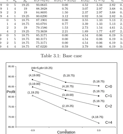
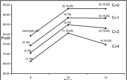
3.1 Base case - Profit vs. correlation . . . 51
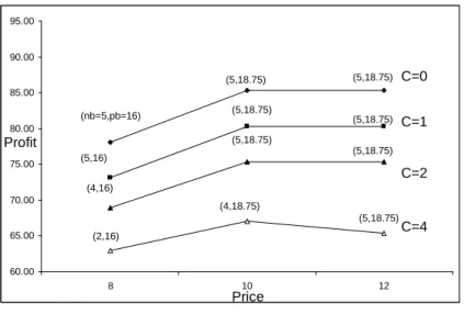
3.2 Profit vs. product price for ρ = −0.9 . . . . 53
3.3 Profit vs. product price for ρ = 0 . . . 53
3.4 Profit vs. product price for ρ = 0.9 . . . 54
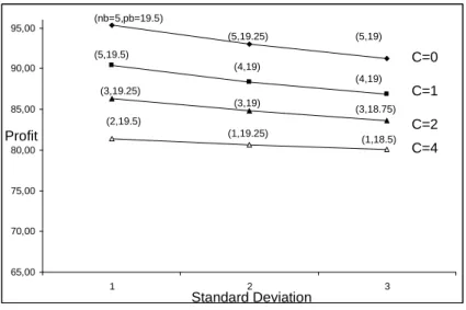
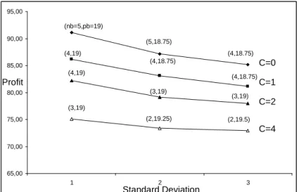
3.5 Profit vs. standard deviation for ρ = −0.9 . . . . 55
3.6 Profit vs. standard deviation for ρ = 0 . . . 56
3.7 Profit vs. standard deviation for ρ = 0.9 . . . 56
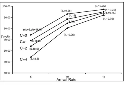
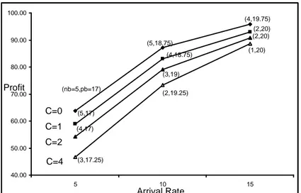
3.8 Profit vs. arrival rate for ρ = −0.9 . . . . 57
3.9 Profit vs. arrival rate for ρ = 0 . . . 58
3.10 Profit vs. arrival rate for ρ = 0.9 . . . 58
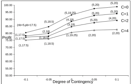
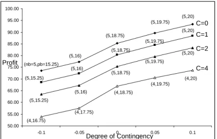
3.11 Profit vs. degree of contingency for ρ = −0.9 . . . 60
3.12 Profit vs. degree of contingency for ρ = 0 . . . 60
3.13 Profit vs. degree of contingency for ρ = 0.9 . . . 61
2.1 Cases of realizations to derive the expected profit . . . 29
3.1 Base case . . . 51
A.1 The impact of product prices on the expected profit . . . 66 A.2 The impact of initial inventory levels on the expected profit . . . 67 A.3 The impact of variance of reservation price distributions on the
expected profit . . . 68 A.4 The impact of arrival rate on the expected profit . . . 69 A.5 The impact of degree of contingency on the expected profit for
ρ = −0.9 . . . 70 A.6 The impact of degree of contingency on the expected profit for ρ = 0 70 A.7 The impact of degree of contingency on the expected profit for
ρ = 0.9 . . . 71
INTRODUCTION AND
LITERATURE REVIEW
1.1
Introduction
One of the main objectives of a firm is to maximize its profits. Profits can be increased through decreasing costs or increasing revenues or both. While most of the operational activities of a firm and academic literature in operations research focus on reduction of costs, significant profit improvements are also possible by managing demand and increasing revenue. Recently, several industries and many researchers are turning their attention to the demand side of the equation under the concept of Yield Management.
Yield Management, also known as Revenue Management, is described as “the process of managing the sales of perishable assets by controlling price and inven-tory so as to maximize profit”(Swann [26]). In this study we incorporate product bundling to the practice of Yield Management. We consider the optimal bun-dle pricing of two products that face stochastic demand during a finite selling horizon.
We consider the bundle formation and pricing problem of a retailer that sells 1
two products facing random demand, under inventory constraints over a finite selling horizon. Before providing a more detailed description of our model and findings we would like to introduce and discuss main concepts related to revenue management and pricing.
The revenue management literature is also referred to as Perishable Asset Revenue Management (PARM) by Weatherford and Bodily [29]. Some examples of perishable goods are airline seats, hotel rooms, seasonal and fashion goods, high technology goods, seats for the theater and sporting events and traffic on network lines. The main characteristics of Revenue Management given by Swann [26] are listed as:
• Limited Capacity: The capacity of the firm is considered limited since extra capacity has a high cost and replenishment takes long time. It is also referred to as “fixed number of product units”.
• Market Segmentation: A company can differentiate the product’s markets via timing of purchase, timing of delivery, etc.
• Perishable Inventory: Products considered in revenue management perish after a specific date.
• Product Sold in Advance: Time of purchase is often used to differentiate products and as a result, in the airline case, the firm should decide the number of seats reserved for low prices and the date of offering only high price seats.
• Variable Demand: Demand varies seasonally, weekly or even daily for prod-ucts. Revenue management is used to smooth the demand variability. As an example, increasing the price during periods of high demand and decreasing the price during periods of low demand can smooth the demand.
By the help of fast and cheap electronic communication and internet, dy-namic pricing is now easily applicable. Companies that successfully implement dynamic pricing to match their and demand include fashion retailer Marks and
Spencer that offers markdowns for its swimsuits before the end of summer season. Delta Airlines offers last-minute cheap tickets to capture the customers with low reservation prices. They categorize fares as five groups (First, Business, Flexible, Discounted, Deeply-discounted). Low fares have more restrictions. (You cannot change your flight date or you can with high penalties compared to others). As the airplane’s seat capacity is fixed, when to offer those tickets and with what price is a valuable research area of dynamic pricing.
Now we review the general pricing concepts.
Noble and Gruca [20] classify the existing theoretical pricing research into a two level framework for industrial goods pricing. The first level consists of four pricing situations: New Product, Competitive, Product Line and Cost-based and the second level contains the pricing strategies appropriate for those situations. The pricing environments and the corresponding strategies are briefly explained below:
1) New Product pricing applies to the early life of a product. Strategies of new product pricing are listed as:
a) Price Skimming: The initial price is set high and systematically reduced over time. Customers expect prices to eventually fall. The main objective is to attract customers who are insensitive to the initial high price. After this segment gets saturated, the price is lowered to increase the demand of the product.
b) Penetration Pricing: In this strategy, the price of the product is set low. The aim is to accelerate the product adoption among customers.
c) Experience Curve Pricing: The initial price is set low again to increase the volume of production and reduce costs through accumulated experience. As a result the unit product cost will be down.
2) Competitive pricing is used when pricing decision is given considering the pricing decisions of competitors. The employed strategies are:
others in the industry will apply price adjustments in the similar direction. In general, the price of an identical product is higher if the leader company sells it due to the brand advantage.
b) Parity Pricing: The firm matches the price set by the overall market or the price leader firm.
c) Low Price Supplier : The firm sets the price lower than its competitors and it aims to have higher demand than the others.
3) Product Line pricing is appropriate when the price of the core product is influenced by the other related products or services of the same company. The pricing strategies are:
a) Complementary Product Pricing: The price of the core product is set low and the complementary items such as accessories, supplies, spare parts, services etc. have prices with a higher premium.
b) Price Bundling: The product is offered as a part of a bundle that contains several products, usually at a total price that gives customers an attractive savings over the sum of individual products.
c) Customer Value Pricing: One version of the product is offered at a very competitive price level; however the product contains fewer features than the main version.
4) Cost-based pricing focuses on the internal costs of the firm including fixed and variable costs and contribution margins.
As mentioned before, bundling is an effective tool for pricing. Bundling does not have a consistent and universally accepted definition. Adams and Yellen [1] define bundling as “selling goods in package” and Guiltinan [13] defines it as “the practice of marketing two or more products and/or services in a single package for a special price”. The definition by Stremersch and Tellis [25] is the “sale of two or more separate products in one package”. They consider separate products as products with separate markets exist and products include both
goods and services. A well-known example of bundling is encountered at fast food restaurants. Burger King’s Whopper Menu contains a big Whopper, fried potatoes and a bottle of Coke. Offering a hotel room and a breakfast is another bundling practice applied in the service industry. Two-way tickets of airline companies are another form of bundling.
Nalebuff [19] provides a good review of bundling concepts and the motivations behind bundling. The author discusses two main reasons for bundling: efficiency reasons and strategic reasons. It is noted that since bundling improves efficiency, even a monopolist firm would have an incentive to offer bundle. The efficiency reasons are listed as:
a) Economies of scale: This is the most apparent reason. For example deliv-ering a suite of software on a single CD is cheaper than sending each one on a separate CD.
b) Improving quality: Through the same example, a suite of software can offer integration and improved functionality.
c) Reducing pricing inefficiencies: The majority of economics literature has developed the theory of how bundling can be used as a price discrimination tool by a multi-good monopoly. (Stigler [24], Adams and Yellen [1], McAffe, McMillan and Whinston [18]). Bundling leads to more homogenous valuations among cus-tomers, thus, the monopolist can capture more consumer surplus. They set the individual prices inefficiently high. Customers evaluate those products with total price, they buy both or neither. Bundling reduces the total price and increases the total profit.
On the other hand, strategic reasons of bundling are given as:
a) Entry deterrence and mitigation of competition: Bundling complementary products prevents the rivals to enter the market. Colgate Motion battery-powered toothbrush and Colgate Total toothpaste are owned by Colgate-Palmolive and they make a promotion bundle to increase the battery-powered toothbrush market share. It is hard for a company, producing toothbrushes, to price as high as
Colgate toothbrushes, since customers buy the complementary toothpaste from Colgate.
b) Gain competitive advantage: Nestle introduced its new product Nescafe Ice through bundling it with its well known product Nescafe. It uses the market power of Nescafe to gain a competitive advantage.
c) Hiding prices: Bundling can hide the individual product prices. It is not easy for a customer to calculate the products’ prices individually.
Bundling is categorized as Product bundling and Price bundling. Stremer-sch and Tellis [25] refer to price bundling as “the sale of two or more separate products in a package at a discount, without any integration of products” and to product bundling as “the integration and sale of two or more separate prod-ucts or services at any price”. Price bundling is a pricing and promotional tool whereas product bundling is more of a strategic tool used to create added value. The integration in product bundling provides added value, such as compactness (multimedia PC), seamless interaction (cars), nonduplicating coverage (all-in-one insurance), reduced risk (mutual fund) or interconnectivity (Bluetooth phone and headset).
Following Adams and Yellen [1], bundling strategies can be classified as pure bundling, mixed bundling and unbundling. Unbundling is “a strategy in which a firm sells the products separately only, not as a bundle”. Pure Bundling is “a strategy in which a firm sells the products only as a bundle but not separately”. Pure bundling is sometimes called tying in the economics and law literature. Mixed Bundling is “a strategy in which a firm sells the products both as a bundle and separately”.
Reservation price is defined as “the maximum price a customer is willing to pay for the product” by Stremersch and Tellis [25]. Purchasing decision is determined by costumer surplus value, which is the total gain of the customer through that purchase (the difference between his reservation price and the product price). If the reservation price is greater than or equal to the product price then he purchases the product, otherwise he does not. In literature, reservation price
behavior of a customer group is modeled as a random variable having mostly a continuous distribution.
Another factor in bundling is the degree of contingency (degree of substi-tutability and complementarity) of the products in the bundle. If the products are substitutable, customers are inclined to buy only one of them at a time. Then, a customer’s reservation price for the bundle would be subadditive (less than the sum of the reservation prices). As an example, different brands of toothpastes Signal White and Colgate Total are substitutes of each other. An increase at the sales amount of one can cause a decrease for the other. When the products are complements, a customer’s reservation price for the bundle is superadditive (more than the sum of the reservation prices). Nestle’s cream, Coffeemate is a comple-ment of Nestle’s coffee, Nescafe. An increase at the sales amount of one product can also cause an increase at the sales of other. As noted in Venkatesh and Kamakura [28], “correlation in reservation prices and the degree of contingency are two distinct notions. While the degree of contingency parameter, θ, captures perceived value enhancement or reduction within each consumer, the correlation in reservation prices of two products, ρ, shows how stand-alone reservation prices relate to each other across consumers”.
Next we want to discuss the pricing and bundling literature related to our study.
1.2
Related Literature
In the literature there are only a few studies combining bundling and pricing issues and mostly these issues are considered separately. Hence, we also divide the literature section into two main parts. The first part focuses on the pricing issues of perishable products and the second part contains bundling and bundle pricing literature.
Pricing Literature
Gallego and van Ryzin [12] is one of the first studies related to dynamic pricing of perishable inventories when demand is price sensitive and the firm’s objective function is to maximize the expected revenues. The authors formulate the problem using intensity control and obtain structural monotonicity results for optimal intensity as a function of the stock level and the length of the selling season. For a particular exponential family of demand functions, they find the optimal pricing policy in closed form. For general demand functions, they find an upper bound on the expected revenue based on analyzing the deterministic version of the problem. They extend their results to the case where demand is compound Poisson; only a finite number of prices is allowed; the demand rate is time dependent; holding cost is incurred and the initial stock level is the decision variable. Feng and Xiao [11] comment on this paper as the model cannot work for short remaining lives and small inventory amounts.
Rajan, Rakesh and Steinberg [21] study the relationship between pricing and ordering decisions of a monopolist retailer facing a known demand function where the products may exhibit physical decay or decrease in market value. They investigate the linear and nonlinear demand cases and provide results on the optimal price changes and optimal cycle length.
Yıldırım, G¨urler and Berk [30] study the dynamic pricing of perishable prod-ucts with random lifetimes and a general distribution. Demand comes from a Poisson Process with a price dependent rate. There is a fixed cost of a price change. They maximize the expected profit with the optimal pricing policy and optimal initial inventory level. They conclude that single price policy results in significantly lower profits through their model.
Feng and Gallego [10] consider the optimal timing of the price change from the initial price to a lower or higher price. They conclude that switching to a lower price as soon as time-to-go falls below a threshold level that depends on the number of stocks at hand. They develop an algorithm to compute the optimal value function and the optimal pricing policy.
Bitran and Caldentey [3] examine the studies on dynamic pricing policies and their relation to Revenue Management. The survey paper is based on a generic Revenue Management problem in which perishable and non-renewable set of resources satisfy stochastic price-sensitive demand processes over a finite period of time.
Bitran and Mondschein [5] study intertemporal pricing policies when selling seasonal products in a retail store. They present a continuous time model where a seller faces a stochastic arrival of customers with different valuation of the product. In this model, they characterize the optimal pricing policies as functions of time and inventory and that model is used as a benchmark for the periodic pricing model. Their model proves the procedures obtained in practice such as retail stores successively discount the product during the season and promote a liquidation sale at the end of the planning horizon. They give some economical insights as uncertainty in the demand of new products leads to higher prices, larger discounts and more unsold inventory.
Bitran, Caldentay and Mondschein [4] propose a methodology to set prices of perishable items in the context of a retail chain with coordinated prices among its stores. The authors formulate a stochastic dynamic programming problem and develop heuristic solutions that approximate optimal solutions.
Federgruen and Heching [9] consider the pricing decision with the inventory decision to maximize profit under a single item, periodic review model. Price dependent stochastic demand function is utilized. They study both finite and infinite horizon models under the assumption that prices can be adjusted ar-bitrarily or that they can only be decreased. Through numerical studies, the authors characterize various qualitative properties of the optimal strategies and corresponding optimal profit values.
Elmegraby and Keskinocak [7] provide a survey of the literature and cur-rent practices about dynamic pricing. Although dynamic pricing is applicable to most markets, their focus is on the dynamic pricing in the presence of inventory considerations.
After giving related pricing literature, now we present a brief discussion on bundle pricing.
Bundling and Bundle Pricing Literature
Stigler [24] is the first study that provides a clear recognition of bundling as a price discrimination tool and is based on stylized examples with a discrete number of customers. In these examples, the reservation values for the components of the bundle are negatively correlated.
Similarly, Adams and Yellen [1] investigate the use of bundling as a price discrimination device. Their study is an important and widely cited essay. They consider a monopolist producing two products with constant unit cost and facing independent demands of customers with different tastes. Customers can buy only one unit of product. The two goods are independent in demand for all customers. Hence customer’s reservation price for one product is independent of the market price of the other. Therefore the maximum amount a customer is willing to pay for a bundle is the sum of the two reservation prices (strict additivity of reservation prices). The reservation prices of the products are negatively correlated. They consider three different sales strategies (unbundling, mixed bundling and pure bundling). They discuss the effects of switching between those strategies. They observe that one strategy generates more profit than others depending on the prevailing level of costs and on the distribution of customers’ reservation prices. They argue that mixed bundling at least dominates pure bundling when the customer’s reservation prices are negatively correlated since the customers with negatively correlated reservation prices prefer the individual products while the others prefer the bundle.
Schamelensee [23] relaxes the negative correlation assumption of Adams and Yellen [1] and adds an additional assumption that customers’ reservation price pairs follow a bivariate normal distribution. Profitability of bundling is examined as a function of production costs, the mean and variance values of customer reser-vation prices for each product and the correlation between the reserreser-vation prices of those products. One of the findings of the study is that even though the profit function is not globally concave, a unique profit-maximizing price always exists,
and it depends on unit cost and the mean of the reservation price distribution. In addition, the effects of changes in standard deviation of reservation price are explored. The author compares mixed bundling case with pure bundling and unbundling cases. It is shown explicitly that pure bundling operates by reducing the effective dispersion of customers’ tastes. As long as the reservation prices are not perfectly correlated, the standard deviation of reservation prices for the bundle is less than the sum of the standard deviations for the two component goods. The increase in profit caused by pure bundling is apparently greater than the fall in consumer surplus, as a result pure bundling increases net welfare. The author mentions that mixed bundling combines the advantages of pure bundling and unbundled sales. Hence mixed bundling is a powerful price discrimination device. A surprising result of analysis is that bundling can be profitable even when demands are uncorrelated or even positively correlated. Two comments are written to this study by Long [17] and Jeuland [16].
Jeuland [16] states that profitability ranking of the bundling strategies (pure bundling, mixed bundling and unbundling) depends on the distribution of the customers’ reservation prices. Long [17] takes a continuous reservation price dis-tribution without restricting it to any particular form for his comments and he states that profitable bundling has a necessary condition of the heterogeneity in customer tastes. If an increase in products’ prices results in individual prod-uct sales, bundling will increase the profit. Another comment of the author is that if the reservation prices of individual products are not positively correlated, bundling increases the profit. The author states that bundling is more powerful as a price discrimination device when the individual products are substitutes of each other.
Salinger [22] provides a graphical analysis of bundling with two products. Additive reservation prices are assumed and main finding of the study is that if bundling does not cause a decrease in cost, then it tends to be profitable when reservation prices are negatively correlated. However if it lowers cost and costs are higher than reservation prices, bundling is profitable when demands for the components are highly positively correlated and component costs are high.
Telser [27] stresses the importance of complementarity between products as a source for bundling. Complementarity between components yields a valuation for the bundle which is super-additive, and this clearly enhances the chances that bundling is profitable.
These early studies do not focus on optimizing bundle prices. Hanson and Martin [14] broaden the bundling studies to find an optimal bundle price to maximize the profit. They investigate how a single monopolist firm, facing a segmented customer demand and product specific cost, can determine optimal product line selection and pricing. They relax the strict additivity of reservation prices. Their formulated problem is a deterministic mixed integer linear pro-gramming model. Deciding optimal number of components included in a bundle is exponentially growing problem as the number of possible components in a prod-uct line increases. Through their computational studies, they give an algorithm for deciding the optimal contents of bundles and their prices.
Stremersch and Tellis [25] combine the bundling concepts referred in market-ing, economics, law and engineering literature into the same terminology. There-fore they remove the inconsistencies and ambiguity in the use of terms. The article clearly and consistently defines the bundling terms and enables a compre-hensive classification of bundling strategies. They give twelve propositions that suggest which bundling strategy is optimal in various contexts.
Ernst and Kouvelis [8] study a newsboy type modeling framework, the com-mon practice of retail firms to sell products not only as independent items but also as part of a bundle. They study a problem similar to ours, in which their focus is the inventory decisions, taking the price set as a given parameter. They also examine the switching between the individual products and the packaged good in the stock out situations. Through the numerical studies, they provide some economical insights. Positive correlation of original demands favors increased stocking levels of a multi-product package, while negative correlation tends to have opposite effect. Demand correlation of individual items and bundle, either positive or negative, results in higher profitability of the inventory system as compared to the uncorrelated case. The higher the negative correlation of the
original demands, the more profitable the inventory system. The stronger the substitution pattern, the higher the optimal stocking level of bundle.
Bulut, Gurler and Sen [6] study the single period pricing of two perishable products which are sold individually and as a bundle. Their customer demand has a Poisson distribution with a price dependent arrival rate. Assuming a general reservation prices distribution, they determine the optimal product prices that maximize the expected revenue. They also compare the performance of three bundling strategies under different conditions such as different reservation price distributions, demand arrival rates and starting inventory levels. Their numer-ical study demonstrates that, when individual product prices are fixed to high values, the expected revenue is a decreasing function of the correlation coeffi-cient, while for low prices the expected revenue is an increasing function of the correlation coefficient. They indicate that, bundling is least effective in case of limited supply and their numerical studies show that the mixed bundling strat-egy outperforms the others, especially when the customer reservation prices are negatively correlated.
In the next section we will give the scope and the motivation of our study.
1.3
Scope of Our Study
Most of the studies done in the bundling literature search for the conditions and strategies where bundling is profitable. These studies usually assume that the products are available in unlimited amounts and the prices are fixed. However, in real life, supply may be constrained and retailers have control over prices. This gap in the literature has motivated our study.
Specifically, we consider a retail firm that sells two types of perishable products over a finite selling season. The starting inventory levels of these two products are fixed and at the beginning of the season, the retailer uses all or a portion of these initial stocks to form product bundles. The retailer then sells the bundles as well as the individual products (mixed bundling) by charging fixed prices over
the selling season. We determine the optimal number of product bundles that the retailer should form and the optimal individual and bundle prices that the retailer should charge so as the maximize his expected profit over the selling season. No replenishments are allowed during the selling season.
As previously explained nearly all bundling papers investigate the performance of pure and mixed bundling strategies. We also give similar strategy comparisons and give some managerial insights about inventory and pricing decisions under bundling.
In our model we consider product bundling and assume that bundles are formed at the beginning of the selling horizon and separation of bundles into individual items is not allowed. We also investigate the effect of cost of forming bundles, as these costs could be non negligible in some industries. For example, combining separate PC components into a PC requires technicians to work on, which adds a labor cost to bundling (See Ansari et al. [2] for a model to determine the number of bundles to be formed).
Customer arrivals to the store follow a Poisson Process with a constant arrival rate and their choice of individual products or the product bundle is governed by their reservation prices. “Posted” product prices are used which means prices are known by the customers, however they do not know the available inventory before they actually arrive at the store. When they arrive, if their preferred product do not available, they may switch to another product or not made purchase. These switching probabilities are related to the reservation prices.
1.4
Summary of Our Results
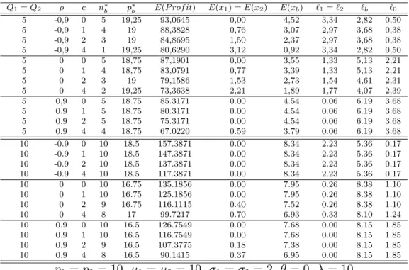
In our numerical study we investigate the effects of various factors on our model, such as the correlation between the reservation price distributions, the variance of the reservation price distributions, initial inventory levels, the unit bundle formation cost, and the intensity of the customer arrivals. We also consider the effects of the degree of product complementarity and substitutability, also known
as the degree of contingency.
We observe from the results of our numerical study that the expected profit decreases as the correlation coefficient increases and increase in bundling cost lowers the profit. With negative correlation, bundling cost has a significant im-pact on the number of bundles formed. However with positive correlation, this effect is negligible.
When the product prices are below the mean value of the reservation price dis-tribution, the optimal bundle price is the maximum of the possible bundle prices, the retailer sells individual products as well as the bundle (mixed bundling). When the individual products are high, the retailer charges a bundle price such that only bundles are sold (pure bundling).
The expected profit and the optimal number of bundles formed decreases as the variance of the reservation price distribution increases. The optimal bun-dle price has different behavior with respect to the correlation coefficient. For negative correlation, optimal bundle price decreases as the standard deviation in-creases. However for positive correlation, the optimal bundle price is an increasing function of the standard deviation. For the uncorrelated case, the optimal bundle price is a decreasing function of the standard deviation for small bundling cost values and it is an increasing function for large bundling cost values.
When the initial inventory levels are high, the retailer reduces bundle price and also offers more bundles for sale as the customer arrival rate is constant. The expected profit is an increasing function of the arrival rate. The number of bundle sales decreases and the number of individual product sales increases when the arrival rate increases since the need for bundling decreases; the retailer can easily sell its products individually.
Finally we perform analysis to investigate the impact of product substitutabil-ity and complementarsubstitutabil-ity. As stated before the products are substitutable when the degree of contingency, θ < 0 (bundle reservation price is subadditive) and complementary when the degree of contingency, θ > 0 (bundle reservation price is superadditive). For all correlation values and bundle formation costs, we see
that the retailer is forming more bundles, or charging higher prices for the bun-dle or both as the degree of contingency increases. As a result, expected profit is an increasing function of degree of contingency. The impact of the degree of contingency is more pronounced when the product prices are uncorrelated and positively correlated.
The rest of the thesis is organized as follows. Chapter 2 formulates the problem investigated and explains the stochastic model used in our study. In Chapter 3 we give results of our numerical studies and in the final chapter we conclude with the discussion of our major findings and the avenues for future research.
MODEL and THE ANALYSIS
As listed in the literature section, most of the studies related to bundle pricing are focused on the determination of optimal inventory levels under a given price set. Our motivation in this study is to combine the pricing decision with the inventory level decision, which is more applicable to the real world business problems. We aim to maximize the expected profit under a mixed bundling strategy for two types of products by determining the optimal number of bundles to be formed and the optimal price set. Our retailer has a finite selling season and a given initial inventory for Product 1 and Product 2. Effect of the bundling cost is also considered in the model.
Before explaining further details of the problem, we mention some of the main assumptions used in our model. The purchasing behaviors of the customers are governed by the reservation prices. Customers decide to buy products by comparing their reservation price and the product price. If their reservation price is higher than the product price they decide to buy the product. Since we do not know the customers’ reservation prices exactly we consider a reservation price distribution to define the customers’ purchasing behavior. We refer the reader to Jedidi and Zhang [15] for further details about estimating the customer reservation prices.
Our model is structured on the main assumption that reservation price for 17
the bundle is the sum of the reservation prices of individual products that form the bundle. This is one of the common assumptions used in the bundling litera-ture such as Adams and Yellen [1], Schmalensee [23] and McAfee [18]. Guiltinan [13] called this assumption as “the assumption of strict additivity”. However Venkatesh and Kamatura [28] added the product substitutability and comple-mentarity to this assumption. If the products that form the bundle are substi-tute products then the reservation price for the bundle is less than the sum of the reservation prices of the individual products as the customers’ willingness to buy both is less. However if the products are complements, customers’ willingness to buy both products at the same time will be higher. At the second part of the study we also investigate the effects of substitution and complementarity among products.
Considering the stock-out situations, we assume the following. When one product incurs shortage, the customer either switches to one of the other products or leaves the store without any purchase. For these cases we assume that switching behavior will follow a Multinomial distribution since there are three possible choices. If two types of products incur shortage, the customer has the alternatives to switch to the available product or to leave without any purchase; therefore binomial distribution is used to calculate the switching probabilities.
2.1
Problem Definition
We consider a retailer with two main product types (Product 1 and Product 2) and a bundle (Product B), formed with the two products, which is sold as a separate product. The aim is to maximize the profit over a single selling season. Stock amounts, Q1 and Q2 of Product 1 and 2 are given and the retailer decides the number of bundles (nb) to be formed with this initial inventory with a unit bundling cost of c. Once the number of bundles to be formed at the beginning of the season, no new bundles are formed and none of them are unbundled to offer individual products during the season.
A customer is allowed to buy only one type of product which means he or she can buy one unit of Product 1, Product 2 or a Bundle but not any combination of products. As in real life situations, a customer can also leave the store without buying any product.
To maximize the profit at the selling season, the prices of Product 1, Product 2 and Bundle (p1, p2 and pb) are optimally decided, where it is assumed that pb ≤ p1+ p2. Product prices are set only at the beginning of the selling season and they are fixed during the period.
Customers’ arrival to the store has a Poisson distribution with a fixed arrival rate, λ customers per season. The decision to buy a product is determined by the comparison of the customer’s reservation price with the product prices. The reservation price for a product is the maximum price that a customer wants to pay for that product. A customer buys a product if its price is less than the customer’s reservation price. Purchase probabilities for Products 1, 2 and the bundle are denoted as m1(p1, p2, pb), m2(p1, p2, pb) and mb(p1, p2, pb) respectively. For brevity, we express mi(p1, p2, pb) as mi for i = 1, 2, b. Then m0 = 1 − m1− m2 − mb is the probability of no purchase. The arrival rates ℓ1, ℓ2 for the two products and the bundle ℓb are then given as ℓi = λ ∗ mi i = 1, 2, b. The difference between the reservation price and the actual price is known as consumer surplus in the economics literature. To maximize the retailer’s profit, consumer surplus should be zero. However, pricing each product differently considering each customer’s reservation price is not an easy task. Therefore bundling can give an alternative way to handle this problem to maximize the profit.
Customers’ reservation prices are random variables. Reservation price of Prod-uct 1 is R1 and reservation price of Product 2 is R2. Mean and variance para-meters of the reservation price distribution are (µ1, σ1) and (µ2, σ2), for Prod-uct 1 and ProdProd-uct 2 respectively. Reservation price of Bundle, Rb, is stated as Rb = R1+ R2.
In the next section, expressions used to calculate expected revenue for a given price set and a fixed number of bundles are presented. These expressions are used to find the optimal number of bundles to be formed and their price to maximize
the expected profit.
2.2
Problem Formulation
2.2.1
Purchasing Probabilities
Let fR1,R2(r1, r2) denotes the joint reservation price density for the two
prod-ucts. When all products are available, purchasing probabilities are calculated by comparing the customer reservation price with the product price. Customer buys either a single product or a bundle or leaves the store without buying any product. Probability expressions of these events are stated below:
Probability of No Purchase: A customer will leave the store without buying any product when his reservation prices for each product and the bundle are lower than their corresponding sales prices. Therefore, the probability of no purchase is stated as,
m0 = P (R1 < p1, R2 < p2, Rb < pb) = P (R1 < p1, R2 < p2, R1+ R2 < pb) = P (R1 < p1, R2 < min {p2, pb− R1}) = Z p1 −∞ Z a1 −∞ fR1,R2(r1, r2)dr1dr2 where a1=min{p2, pb− r1}.
Probability of Purchasing Product 1: Purchase probabilities are calcu-lated by comparing the consumer surplus, which is the difference between the reservation price and the product price. A customer will purchase Product 1 if his surplus from Product 1 is positive and greater than his surplus values from Product 2 and the bundle separately. Thus the probability of purchasing Product 1 is stated as,
= P (R1 > p1, R1− p1 > R2 − p2, R1− p1 > R1+ R2− pb) = P (R1 > p1, R2 < min {R1− p1+ p2, pb− p1}) = Z ∞ p1 Z a2 −∞ fR1,R2(r1, r2)dr1dr2 where a2=min {r1 − p1+ p2, pb− p1} .
Probability of Purchasing Product 2: The probability of purchasing Product 2 is similarly stated as,
m2 = P (R2 > p2, R2− p2 > R1 − p1, R2− p2 > Rb− pb) = P (R2 > p2, R2− p2 > R1 − p1, R2− p2 > R1+ R2− pb) = P (R2 > p2, R1 < min {R2− p2+ p1, pb− p2}) = Z ∞ p2 Z a3 −∞ fR1,R2(r1, r2)dr2dr1 where a3=min {r2 − p2+ p1, pb− p2} .
Probability of Purchasing a Bundle: Using the same reasoning we state the probability of purchasing a bundle as,
mb = P (Rb > pb, Rb− pb > R1− p1, Rb− pb > R2− p2) = P (R1+ R2 > pb, R1+ R2− p2 > R1− p1, R1+ R2− pb > R2− p2) = P (R1 > pb− p2, R2 > max {pb− R1, pb− p1}) = Z ∞ pb−p2 Z ∞ a4 fR1,R2(r1, r2)dr1dr2 where a4=max {pb− r1, pb− p1}
2.2.2
Switching Probabilities
We now consider the situation when one or two product types are not available. One Type of Product Incurs Shortage
Probability of Switching from Product 1 to Bundle or to Product 2
Suppose Product 1 incurs shortage and the customer has the option to switch to the Bundle, Product 2 or to leave without purchase. Let θ1B, θ12 and 1 − θ1B − θ12 be the probability of these events respectively. Since the switching events follow after the first choices of the customers are made, we calculate these probabilities conditional on the event that the first preference of the customer was to buy Product 1. Then we have
θ1B = Pr ( Rb − Pb ≥ R2− p2; Rb ≥ pb R1− p1 ≥ Rb− pb; R1− p1 ≥ R2− p2; R1 ≥ p1 ) = Pr R1+ R2 − pb ≥ R2− p2; R1+ R2 ≥ pb; R1− p1 ≥ R1+ R2− pb; R1− p1 ≥ R2− p2; R1 ≥ p1 /m1 = Pr ( R1 ≥ pb− p2; R2 ≥ pb− R1; pb− p1 ≥ R2; R1− p1+ p2 ≥ R2; R1 ≥ p1 ) /m1 = Pr ( R1 ≥ max (pb− p2, p1) ; min (pb − p1, R1− p1 + p2) ≥ R2 ≥ pb− R1 ) /m1 = Pr ( R1 ≥ max (pb − p2, p1) ; pb− p1 ≥ R2 ≥ pb − R1 ) /m1 = Z ∞ max(pb−p2,p1) Z pb−p1 pb−r1 fR1,R2(r1, r2)dr1dr2/m1 Similarly we have θ12 = Pr ( R2− p2 ≥ Rb − pb; R2 ≥ p2 R1− p1 ≥ Rb− pb; R1 − p1 ≥ R2− p2; R1 ≥ p1 ) = Pr ( R2 − p2 ≥ R1+ R2− pb; R2 ≥ p2; R1− p1 ≥ R1+ R2− pb; R1− p1 ≥ R2 − p2; R1 ≥ p1 ) /m1
= Pr ( pb− p2 ≥ R1; R2 ≥ p2; pb− p1 ≥ R2; p2+ R1− p1 ≥ R2; R1 ≥ p1 ) /m1 = Pr ( pb− p2 ≥ R1 ≥ p1; min(pb− p1, p2+ R1− p1) ≥ R2 ≥ p2 ) /m1 = Pr ( pb− p2 ≥ R1 ≥ p1; p2+ R1− p1 ≥ R2 ≥ p2 ) /m1 = Z pb−p2 p1 Z p2+r1−p1 p2 fR1,R2(r1, r2)dr1dr2/m1
Probability of Switching from Product 2 to Bundle or to Product 1
Similar to the previous case let θ2B, θ21 be the probability of switching to a Bundle or to Product 1 when Product 2 stocks our. We have
θ2B = Pr ( Rb− pb ≥ R1− p1; Rb ≥ pb R2− p2 ≥ Rb− pb; R2− p2 ≥ R1− p1; R2 ≥ p2 ) = Pr R1+ R2− pb ≥ R1− p1; R1+ R2 ≥ pb; R2− p2 ≥ R1 + R2− pb; R2− p2 ≥ R1 − p1; R2 ≥ p2 /m2 = Pr ( R2 ≥ pb− p1; R1 ≥ pb− R2; pb− p2 ≥ R1; R2− p2+ p1 ≥ R1; R2 ≥ p2 ) /m2 = Pr ( R2 ≥ max(pb− p1, p2); min(pb− p2, R2− p2+ p1) ≥ R1 ≥ pb− R2 ) /m2 = Pr ( R2 ≥ max(pb− p1, p2); pb− p2 ≥ R1 ≥ pb− R2 ) /m2 = Z ∞ max(pb−p1,p2) Z pb−p2 pb−r2 fR1,R2(r1, r2)dr2dr1/m2 and θ21 = Pr ( R1− p1 ≥ Rb− pb; R1 ≥ p1 R2− p2 ≥ Rb− pb; R2− p2 ≥ R1− p1; R2 ≥ p2 ) = Pr R1− p1 ≥ R1+ R2− pb; R1 ≥ p1; R2− p2 ≥ R1+ R2− pb; R2− p2 ≥ R1− p1; R2 ≥ p2 /m2
= Pr ( pb − p1 ≥ R2; R1 ≥ p1; pb− p2 ≥ R1; R2− p2+ p1 ≥ R1; R2 ≥ p2 ) /m2 = Pr ( pb− p1 ≥ R2 ≥ p2; R2− p2+ p1 ≥ R1 ≥ p1 ) /m2 = Z pb−p1 p2 Z r2−p2+p1 p1 fR1,R2(r1, r2)dr2dr1/m2
Probability of Switching from Bundle to Product 1 or to Product 2
Now let θB1and θB2be the probability of switching to Product 1 or to Product 2 when Bundle stocks our. We have
θB1 = Pr ( R1− p1 ≥ R2− p2; R1 ≥ p1 Rb − pb ≥ R1− p1; Rb− pb ≥ R2− p2; Rb ≥ pb ) = Pr R1 − p1+ p2 ≥ R2; R1 ≥ p1; R1+ R2− pb ≥ R1− p1; R1+ R2− pb ≥ R2− p2; R1+ R2 ≥ pb /mb = Pr ( R1 − p1+ p2 ≥ R2; R1 ≥ p1; R2 ≥ pb− p1; R1 ≥ pb− p2; R2 ≥ pb− R1 ) /mb = Pr ( R1 ≥ max(p1, pb− p2) R1− p1+ p2 ≥ R2 ≥ max(pb− p1, pb− R1) ) /mb = Pr ( R1 ≥ max(p1, pb− p2) R1− p1+ p2 ≥ R2 ≥ pb− p1 ) /mb = Z ∞ max(p1,pb−p2) Z r1−p1+p2 pb−p1 fR1,R2(r1, r2)dr1dr2/mb and θB2 = Pr ( R2− p2 ≥ R1− p1; R2 ≥ p2 Rb − pb ≥ R1− p1; Rb− pb ≥ R2− p2; Rb ≥ pb ) = Pr R2 − p2+ p1 ≥ R1; R2 ≥ p2; R1+ R2− pb ≥ R1− p1; R1+ R2− pb ≥ R2− p2; R1+ R2 ≥ pb /mb = Pr ( R2 − p2+ p1 ≥ R1; R2 ≥ p2; R2 ≥ pb− p1; R1 ≥ pb− p2; R1 ≥ pb− R2 ) /mb
= Pr ( R2 ≥ max(p2, pb− p1) R2− p2+ p1 ≥ R1 ≥ max(pb− p2, pb− R2) ) /mb = Pr ( R2 ≥ max(p2, pb− p1) R2− p2+ p1 ≥ R1 ≥ pb− p2 ) /mb = Z ∞ max(p2,pb−p1) Z r2−p2+p1 pb−p2 fR1,R2(r1, r2)dr2dr1/mb
Two Types of Products Incur Shortage
Switching probabilities explained in this section are used when dedicated cus-tomer cannot find his preferred product and only one type of the remaining prod-ucts is available. Therefore, customer can decide only to switch to that available product or to leave the store without buying any product.
Product 1 and Product 2 incur shortage: Let θ−
1B, θ −
2B be the probability of switching from Product 1 or Product 2 to Bundle when only Bundle is available. Then we have,
θ− 1B = Pr ( Rb ≥ pb R1− p1 ≥ Rb− pb; R1− p1 ≥ R2− p2; R1 ≥ p1 ) = Pr ( R1+ R2 ≥ pb; R1 − p1 ≥ R1+ R2− pb; R1− p1 ≥ R2− p2; R1 ≥ p1 ) /m1 = Pr ( R2 ≥ pb− R1; pb− p1 ≥ R2; R1− p1+ p2 ≥ R2; R1 ≥ p1 ) /m1 = Pr ( R1 ≥ p1; min(pb− p1, R1− p1+ p2) ≥ R2 ≥ pb− R1 ) /m1 = Z ∞ p1 Z min(pb−p1,r1−p1+p2) pb−r1 fR1,R2(r1, r2)dr1dr2/m1 and θ− 2B = Pr ( Rb ≥ pb R2− p2 ≥ Rb− pb; R2− p2 ≥ R1− p1; R2 ≥ p2 ) = Pr ( R1+ R2 ≥ pb; R2 − p2 ≥ R1+ R2− pb; R2− p2 ≥ R1− p1; R2 ≥ p2 ) /m2
= Pr ( R1 ≥ pb− R2; pb− p2 ≥ R1; R2− p2+ p1 ≥ R1; R2 ≥ p2 ) /m2 = Pr ( R2 ≥ p2 min(R2− p2+ p1, pb − p2) ≥ R1 ≥ pb− R2 ) /m2 = Z ∞ p2 Z min(r2−p2+p1,pb−p2) pb−r2 fR1,R2(r1, r2)dr2dr1/m2
Bundle and Product 2 incur shortage Let θ−
B1, θ −
21 be the probability of switching from Bundle or Product 2 to Product 1 when only Product 1 is available. Then
θ− B1 = Pr ( R1 ≥ p1 Rb− pb ≥ R1− p1; Rb− pb ≥ R2− p2; Rb ≥ pb ) = Pr ( R1 ≥ p1; R1+ R2− pb ≥ R1− p1; R1+ R2− pb ≥ R2− p2; R1+ R2 ≥ pb ) /mb = Pr ( R1 ≥ p1; R2 ≥ pb− p1; R1 ≥ pb − p2; R2 ≥ pb− R1 ) /mb = Pr ( R1 ≥ max(p1, pb − p2) R2 ≥ max(pb− p1, pb− R1) ) /mb = Pr ( R1 ≥ max(p1, pb− p2) R2 ≥ pb− p1 ) /mb = Z ∞ max(p1,pb−p2) Z ∞ pb−p1 fR1,R2(r1, r2)dr1dr2/mb and we have θ− 21 = Pr ( R1 ≥ p1 R2− p2 ≥ Rb − pb; R2− p2 ≥ R1− p1; R2 ≥ p2 ) = Pr ( R1 ≥ p1; R2− p2 ≥ R1+ R2− pb; R2 − p2 ≥ R1− p1; R2 ≥ p2 ) /m2 = Pr ( R1 ≥ p1; pb− p2 ≥ R1; R2 ≥ R1− p1+ p2; R2 ≥ p2 ) /m2 = Pr ( pb− p2 ≥ R1 ≥ p1; R2 ≥ max(R1− p1+ p2, p2) ) /m2
= Pr ( pb− p2 ≥ R1 ≥ p1; R2 ≥ R1− p1 + p2 ) /m2 = Z pb−p2 p1 Z ∞ r1−p1+p2 fR1,R2(r1, r2)dr1dr2/m2
Bundle and Product 1 incur shortage Similar to the previous case let θ−
B2 and θ −
12 be the probability of switching when only Product 2 is available. Then,
θ− B2 = Pr ( R2 ≥ p2 Rb− pb ≥ R1− p1; Rb− pb ≥ R2− p2; Rb ≥ pb ) = Pr ( R2 ≥ p2; R1+ R2− pb ≥ R1− p1; R1+ R2− pb ≥ R2− p2; R1+ R2 ≥ pb ) /mb = Pr ( R2 ≥ p2; R2 ≥ pb− p1; R1 ≥ pb − p2; R1 ≥ pb− R2 ) /mb = Pr ( R2 ≥ max(p2, pb− p1); R1 ≥ max(pb− p2, pb− R2) ) /mb = Pr ( R2 ≥ max(p2, pb− p1); R1 ≥ pb− p2 ) /mb = Z ∞ pb−p2 Z ∞ max(p2,pb−p1) fR1,R2(r1, r2)dr1dr2/mb and θ− 12 = Pr ( R2 ≥ p2 R1− p1 ≥ Rb − pb; R1− p1 ≥ R2− p2; R1 ≥ p1 ) = Pr ( R2 ≥ p2; R1− p1 ≥ R1+ R2− pb; R1 − p1 ≥ R2− p2; R1 ≥ p1 ) /m1 = Pr ( R2 ≥ p2; pb− p1 ≥ R2; R1 ≥ R2− p2+ p1; R1 ≥ p1 ) /m1 = Pr ( pb− p1 ≥ R2 ≥ p2; R1 ≥ max(R2− p2+ p1, p1) ) /m1 = Pr ( pb− p1 ≥ R2 ≥ p2; R1 ≥ R2− p2 + p1 ) /m1
= Z pb−p1 p2 Z ∞ r2−p2+p1 fR1,R2(r1, r2)dr2dr1/m1
After explaining the purchase and switching probability calculations, we explain the probability calculations for different sale realizations in the next section.
2.3
Sales Probabilities and the Objective
Func-tion
Recall that Q1 and Q2 are the initial inventory levels of Product 1 and Product 2, respectively. Let nb be the number of bundles formed and ni i = 1, 2 be the remaining units of Product i, with n1 = Q1− nb and n2 = Q2− nb.
Also let X1, X2 and Xb be the number of dedicated customers for Product 1, Product 2 and the Bundle respectively. We also have the random variables corre-sponding to the number of dedicated customers that switch from one product to another. These variables are denoted as Xij, where i is the dedicated customer’s product type (first preference) and j is the type of the product that the customer switches to (substitutes for i).
The realized values of these random variables will be denoted by x1, x2, xb, x1b, x12, x2b, x21, xb1 and xb2. Let P x1, x2, xb, x1b, x12, x2b, x21, xb1, xb2 ! = P X1 = x1, X2 = x2, Xb = xb, X1b = x1b, X12 = x12, X2b = x2b, X21= x21, Xb1= xb1, Xb2= xb2
denote the joint probability mass function of those random variables. Note that for certain realizations we only need joint marginal probability mass function of only a subset of these variables.
When all dedicated demand can be satisfied, due to the independency property of the Poisson processes, we have
Case 1: Nothing incurs shortage Case 2: Bundle incurs shortage
a) All excess demand of the Bundle is satisfied
b) Product 1 incurs shortage with the excess bundle demand c) Product 2 incurs shortage with the excess bundle demand d) Both products incur shortage with the excess bundle demand Case 3: Product 1 incurs shortage
a) All excess demand of Product 1 is satisfied
b) Product 2 incurs shortage with the excess demand of Product 1 c) Bundle incurs shortage with the excess demand of Product 1
d) Product 2 and Bundle incur shortage with the excess demand of Product 1 Case 4: Product 2 incurs shortage
a) All excess demand of Product 2 is satisfied
b) Product 1 incurs shortage with the excess demand of Product 2 c) Bundle incurs shortage with the excess demand of Product 2
d) Product 1 and Bundle incur shortage with the excess demand of Product 2 Case 5: Product 1 and the Bundle incur shortage
a) All excess demand of Product 1 and the Bundle are satisfied
b) Product 2 incurs shortage with the excess demand of Product 1 and the Bundle Case 6: Product 2 and the Bundle incur shortage
a) All excess demand of Product 2 and the Bundle are satisfied
b) Product 1 incurs shortage with the excess demand of Product 2 and the Bundle Case 7: Product 1 and Product 2 incur shortage
a) All excess demand of the products are satisfied from the Bundle b) Bundle incurs shortage with the excess demand of two products Case 8: All products incur shortage
Table 2.1: Cases of realizations to derive the expected profit
where Xi has a Poisson distribution with rate ℓi = λ ∗ mi, i = 1, 2, b.
For the derivation of the expected profit, π, there are eight possible realization cases when the initial choices are only considered. After this first classification, sub-cases are defined to include the switching customer realizations. All realiza-tion cases are listed in Table 2.1.
Case 1: Nothing incurs shortage (x1 ≤ n1, x2 ≤ n2, xb ≤ nb)
Expected profit in the region where all customers are satisfied by their first choice products is given by π1 which is
π1 = n1 X x1=0 n2 X x2=0 nb X xb=0 (x1p1+ x2p2+ xbpb− nbc) P (x1, x2, xb) = n1 X x1=0 n2 X x2=0 nb X xb=0 (x1p1+ x2p2+ xbpb− nbc)e −ℓ1ℓx1 1 x1! e−ℓ2ℓx2 2 x2! e−ℓbℓxb b xb!
Case 2: Bundle incurs shortage (x1 ≤ n1, x2 ≤ n2, xb > nb)
Initial demand for the bundle is more than the available stock but initial demands for Product 1 and Product 2 are satisfied from the stocks. Excess demand of the Bundle customers can result in four sub-cases.
(a) All excess demand of the Bundle is satisfied
Let xb − nb be the number of excess bundle customers. In this case, xb− nb units are satisfied from the excess inventories of Product 1 and Product 2. That is, we have x1+ xb1 ≤ n1 , x2 + xb2 ≤ n2, x1 ≤ n1, x2 ≤ n2 , xb > nb and the contribution of this case to the total expected profit is given by:
π2a = n1 X x1=0 n2 X x2=0 ∞ X xb=nb xb−nb X xb1=0 xb−nb−xb1 X xb2=0 ((x1+ xb1)p1+ (x2+ xb2)p2+ nbpb − nbc) P (x1, x2, xb, xb1, xb2) = n1 X x1=0 n2 X x2=0 ∞ X xb=nb xb−nb X xb1=0 xb−nb−xb1 X xb2=0 ((x1+ xb1)p1+ (x2+ xb2)p2+ nbpb − nbc) e−ℓ1ℓx1 1 x1! e−ℓ2ℓx2 2 x2! e−ℓbℓxb b xb! (xb− nb)! xb1!xb2!xb0!(θ − B1)xb1(θ − B2)xb2(θ − B0)xb0 where xb0= xb− nb− xb1− xb2 and θB0− = 1 − θ − B1− θ − B2
(b) Product 1 incurs shortage with the excess bundle demand
In this case, original demand for Product 1 is satisfied but the left over is not sufficient to satisfy the overflow from the Bundle customers. All demands for Product 2 are satisfied from the stock. For this case we have x1+ xb1 > n1 , x2+ xb2 ≤ n2, x1 ≤ n1, x2 ≤ n2 , xb > nb and the contribution is given by:
π2b = n1 X x1=0 n2 X x2=0 ∞ X xb=nb xb−nb X xb1=n1−x1 xb−nb−xb1 X xb2=0 (n1p1+ (x2+ xb2)p2+ nbpb− nbc) P (x1, x2, xb, xb1, xb2) = n1 X x1=0 n2 X x2=0 ∞ X xb=nb xb−nb X xb1=n1−x1 xb−nb−xb1 X xb2=0 (n1p1+ (x2+ xb2)p2+ nbpb− nbc) e−ℓ1ℓx1 1 x1! e−ℓ2ℓx2 2 x2! e−ℓbℓxb b xb! (xb− nb)! xb1!xb2!xb0!(θ − B1)xb1(θ − B2)xb2(θ − B0)xb0
(c) Product 2 incurs shortage with the excess bundle demand
This case is similar to the above case, except that Product 2 incurs shortage. Hence we have x1+ xb1 ≤ n1 , x2+ xb2 > n2, x1 ≤ n1, x2 ≤ n2 , xb > nb and the contribution is given by:
π2c = n1 X x1=0 n2 X x2=0 ∞ X xb=nb xb−nb X xb1=0 xb−nb−xb1 X xb2=n2−x2 ((x1+ xb1)p1 + n2p2+ nbpb− nbc) P (x1, x2, xb, xb1, xb2) = n1 X x1=0 n2 X x2=0 ∞ X xb=nb xb−nb X xb1=0 xb−nb−xb1 X xb2=n2−x2 ((x1+ xb1)p1 + n2p2+ nbpb− nbc) e−ℓ1ℓx1 1 x1! e−ℓ2ℓx2 2 x2! e−ℓbℓxb b xb! (xb− nb)! xb1!xb2!xb0!(θ − B1) xb1(θ− B2) xb2(θ− B0) xb0
(d) Both products incur shortage with the excess bundle demand
In this case the excess inventories of Product 1 and Product 2 are not sufficient to satisfy the overflow demand from the bundle customers. That is, we have x1+ xb1 > n1 , x2+ xb2 > n2, x1 ≤ n1, x2 ≤ n2 , xb > nb and π2d = n1 X x1=0 n2 X x2=0 ∞ X xb=nb xb−nb X xb1=n1−x1 xb−nb−xb1 X xb2=n2−x2 (n1p1+ n2p2+ nbpb− nbc)
P (x1, x2, xb, xb1, xb2) = n1 X x1=0 n2 X x2=0 ∞ X xb=nb xb−nb X xb1=n1−x1 xb−nb−xb1 X xb2=n2−x2 (n1p1+ n2p2+ nbpb− nbc) e−ℓ1ℓx1 1 x1! e−ℓ2ℓx2 2 x2! e−ℓbℓxb b xb! (xb− nb)! xb1!xb2!xb0!(θ − B1)xb1(θ − B2)xb2(θ − B0)xb0
Expected profit for the Case 2 is calculated as π2 = π2a+ π2b+ π2c+ π2d Case 3: Product 1 incurs shortage (x1 > n1, x2 ≤ n2, xb ≤ nb)
Initial demand for Product 1 is more than the available stock but initial demands for Product 2 and the Bundle are satisfied from the stocks. Excess demand of Product 1 customers can result in four sub-cases.
(a) All excess demand of Product 1 is satisfied
Demands for Product 2 and Bundle are satisfied including the switching cus-tomers from Product 1. We have x2+ x12 ≤ n2, xb+ x1b ≤ nb, x1 > n1, x2 ≤ n2, xb ≤ nb and π3a = ∞ X x1=n1 n2 X x2=0 nb X xb=0 x1−n1 X x12=0 x1−n1−x12 X x1b=0 (n1p1+ (x2+ x12)p2+ (xb+ x1b)pb− nbc) P (x1, x2, xb, x12, x1b) = ∞ X x1=n1 n2 X x2=0 nb X xb=0 x1−n1 X x12=0 x1−n1−x12 X x1b=0 (n1p1+ (x2+ x12)p2+ (xb+ x1b)pb− nbc) e−ℓ1ℓx1 1 x1! e−ℓ2ℓx2 2 x2! e−ℓbℓxb b xb! (x1− n1)! x12!x1b!x10!(θ − 12)x12(θ − 1B) x1b(θ− 10)x10 where x10= x1− n1− x12− x1b and θ10− = 1 − θ − 12− θ − 1B
(b) Product 2 incurs shortage with the excess demand of Product 1
In this case, we have x2+ x12 > n2, xb+ x1b≤ nb, x1 > n1, x2 ≤ n2, xb ≤ nb and π3b = ∞ X x1=n1 n2 X x2=0 nb X xb=0 x1−n1 X x12=n2−x2 x1−n1−x12 X x1b=0 (n1p1+ n2p2+ (xb+ x1b)pb− nbc)
P (x1, x2, xb, x12, x1b) = ∞ X x1=n1 n2 X x2=0 nb X xb=0 x1−n1 X x12=n2−x2 x1−n1−x12 X x1b=0 (n1p1+ n2p2+ (xb+ x1b)pb− nbc) e−ℓ1ℓx1 1 x1! e−ℓ2ℓx2 2 x2! e−ℓbℓxb b xb! (x1 − n1)! x12!x1b!x10!(θ − 12)x12(θ−1B)x1b(θ − 10)x10
(c) Bundle incurs shortage with the excess demand of Product 1
Hence the overflow Product 1 customers to Bundle are not satisfied with the excess stock of the bundle, but all demands for Product 2 are satisfied from the stock. Then, x2+ x12 ≤ n2, xb+ x1b> nb, x1 > n1, x2 ≤ n2, xb ≤ nb and
π3c = ∞ X x1=n1 n2 X x2=0 nb X xb=0 x1−n1 X x12=0 x1−n1−x12 X x1b=nb−xb (n1p1+ (x2+ x12)p2+ nbpb − nbc) P (x1, x2, xb, x12, x1b) = ∞ X x1=n1 n2 X x2=0 nb X xb=0 x1−n1 X x12=0 x1−n1−x12 X x1b=nb−xb (n1p1+ (x2+ x12)p2+ nbpb − nbc) e−ℓ1ℓx1 1 x1! e−ℓ2ℓx2 2 x2! e−ℓbℓxb b xb! (x1− n1)! x12!x1b!x10!(θ − 12)x12(θ − 1B)x1b(θ − 10)x10
(d) Product 2 and Bundle incur shortage with the excess demand of Product 1 In this case the overflows to Product 2 and the Bundle from Product 1 are not satisfied by the excess inventories. That is, x2 + x12 > n2, xb + x1b > nb, x1 > n1, x2 ≤ n2, xb ≤ nb and π3d = ∞ X x1=n1 n2 X x2=0 nb X xb=0 x1−n1 X x12=n2−x2 x1−n1−x12 X x1b=nb−xb (n1p1+ n2p2+ nbpb− nbc) P (x1, x2, xb, x12, x1b) = ∞ X x1=n1 n2 X x2=0 nb X xb=0 x1−n1 X x12=n2−x2 x1−n1−x12 X x1b=nb−xb (n1p1+ n2p2+ nbpb− nbc) e−ℓ1ℓx1 1 x1! e−ℓ2ℓx2 2 x2! e−ℓbℓxb b xb! (x1− n1)! x12!x1b!x10!(θ − 12)x12(θ1B− )x1b(θ − 10)x10
Case 4: Product 2 incurs shortage (x1 ≤ n1, x2 > n2, xb ≤ nb)
This case is similar to case 3, so we directly write the expressions of sub-cases. (a) All excess demand of Product 2 is satisfied
We have x1+ x21≤ n1, xb+ x2b≤ nb, x1 ≤ n1, x2 > n2, xb ≤ nb and π4a = n1 X x1=0 ∞ X x2=n2 nb X xb=0 x2−n2 X x21=0 x2−n2−x21 X x2b=0 ((x1+ x21)p1+ n2p2+ (xb+ x2b)pb− nbc) P (x1, x2, xb, x21, x2b) = n1 X x1=0 ∞ X x2=n2 nb X xb=0 x2−n2 X x21=0 x2−n2−x21 X x2b=0 ((x1+ x21)p1+ n2p2+ (xb+ x2b)pb− nbc) e−ℓ1ℓx1 1 x1! e−ℓ2ℓx2 2 x2! e−ℓbℓxb b xb! (x2− n2)! x21!x2b!x20! (θ− 21)x21(θ − 2B)x2b(θ − 20)x20 where x20= x2− n2− x21− x2b and θ20− = 1 − θ − 21− θ − 2B
(b) Product 1 incurs shortage with the excess demand of Product 2 x1+ x21> n1, xb+ x2b≤ nb, x1 ≤ n1, x2 > n2, xb ≤ nb π4b = n1 X x1=0 ∞ X x2=n2 nb X xb=0 x2−n2 X x21=n1−x1 x2−n2−x21 X x2b=0 (n1p1+ n2p2+ (xb+ x2b)pb− nbc) P (x1, x2, xb, x21, x2b) = n1 X x1=0 ∞ X x2=n2 nb X xb=0 x2−n2 X x21=n1−x1 x2−n2−x21 X x2b=0 (n1p1+ n2p2+ (xb+ x2b)pb− nbc) e−ℓ1ℓx1 1 x1! e−ℓ2ℓx2 2 x2! e−ℓbℓxb b xb! (x2 − n2)! x21!x2b!x20!(θ − 21)x21(θ−2B)x2b(θ − 20)x20
(c) Bundle incurs shortage with the excess demand of Product 2 x1+ x21≤ n1, xb + x2b > nb, x1 ≤ n1, x2 > n2, xb ≤ nb π4c = n1 X x1=0 ∞ X x2=n2 nb X xb=0 x2−n2 X x21=0 x2−n2−x21 X x2b=nb−xb ((x1+ x21)p1+ n2p2+ nbpb − nbc) P (x1, x2, xb, x21, x2b)
= n1 X x1=0 ∞ X x2=n2 nb X xb=0 x2−n2 X x21=0 x2−n2−x21 X x2b=nb−xb ((x1+ x21)p1+ n2p2+ nbpb − nbc) e−ℓ1ℓx1 1 x1! e−ℓ2ℓx2 2 x2! e−ℓbℓxb b xb! (x2− n2)! x21!x2b!x20! (θ− 21)x21(θ − 2B)x2b(θ − 20)x20
(d) Product 1 and Bundle incur shortage with the excess demand of Product 2 x1+ x21> n1, xb+ x2b> nb, x1 ≤ n1, x2 > n2, xb ≤ nb π4d = n1 X x1=0 ∞ X x2=n2 nb X xb=0 x2−n2 X x21=n1−x1 x2−n2−x21 X x2b=nb−xb (n1p1+ n2p2+ nbpb− nbc) P (x1, x2, xb, x21, x2b) = n1 X x1=0 ∞ X x2=n2 nb X xb=0 x2−n2 X x21=n1−x1 x2−n2−x21 X x2b=nb−xb (n1p1+ n2p2+ nbpb− nbc) e−ℓ1ℓx1 1 x1! e−ℓ2ℓx2 2 x2! e−ℓbℓxb b xb! (x2− n2)! x21!x2b!x20!(θ − 21)x21(θ − 2B) x2b(θ− 20)x20
Expected profit for the Case 4 is calculated as π4 = π4a+ π4b+ π4c+ π4d
Case 5: Product 1 and the Bundle incur shortage (x1 > n1, x2 ≤ n2,
xb > nb)
Initial demands for Product 1 and the Bundle are greater than the respective stock amounts and only initial demand for Product 2 is satisfied from the stock. Excess demands of Product 1 and the Bundle result in two sub-cases.
(a) All excess demand of Product 1 and the Bundle are satisfied
Demand for Product 2 is satisfied including the switching customers from Product 1 and the Bundle. That is, we have x2 + x12 + xb2 ≤ n2, x1 > n1, x2 ≤ n2, xb > nb and π5a = ∞ X x1=n1 n2 X x2=0 ∞ X xb=nb x1−n1 X x12=0 xb−nb X xb2=0 (n1p1+ (x2 + x12+ xb2)p2 + nbpb− nbc) P (x1, x2, xb, x12, xb2) = ∞ X x1=n1 n2 X x2=0 ∞ X xb=nb x1−n1 X x12=0 xb−nb X xb2=0 (n1p1+ (x2 + x12+ xb2)p2 + nbpb− nbc)
e−ℓ1ℓx1 1 x1! e−ℓ2ℓx2 2 x2! e−ℓbℓxb b xb! x1− n1 + x12− 1 x1− n1− 1 ! (θ12)x1−n1 (1 − θ12)x12 xb − nb+ xb2− 1 xb − nb− 1 ! (θB2)xb−nb (1 − θB2)xb2
(b) Product 2 incurs shortage with the excess demand of Product 1 and the Bundle
Initial Product 2 demand is satisfied but excess demand from Product 1 and Bundle cannot be satisfied with the Product 2 stock. We have x2+x12+xb2> n2, x1 > n1, x2 ≤ n2, xb > nb and π5b = ∞ X x1=n1 n2 X x2=0 ∞ X xb=nb X x12,xb2: x12+xb2≥n2−x2 (n1p1+ n2p2+ nbpb− nbc) P (x1, x2, xb, x12, xb2) = ∞ X x1=n1 n2 X x2=0 ∞ X xb=nb X x12,xb2: x12+xb2≥n2−x2 (n1p1+ n2p2+ nbpb− nbc) e−ℓ1ℓx1 1 x1! e−ℓ2ℓx2 2 x2! e−ℓbℓxb b xb! x1− n1+ x12− 1 x1− n1− 1 ! (θ12)x1−n1 (1 − θ12)x12 xb− nb+ xb2− 1 xb− nb − 1 ! (θB2)xb−nb (1 − θB2)xb2
Expected profit for the Case 5 is calculated as π5 = π5a+ π5b
Case 6: Product 2 and the Bundle incur shortage (x1 ≤ n1, x2 > n2,
xb > nb)
Initial demand for Product 2 and Bundle are greater than their respective stock amounts and only initial Product 1 demand is satisfied from the stock. We have again two sub-cases: