ORIGINAL PAPER
AN OPERATIONAL MATRIX METHOD TO SOLVE LINEAR
FREDHOLM-VOLTERRA INTEGRO-DIFFERENTIAL EQUATIONS
YALCIN OZTURK1
_________________________________________________ Manuscript received: 06.03.2020; Accepted paper: 04.04.2020;
Published online: 30.06.2020.
Abstract. In this paper, it is an operational matrix method associating Chebyshev
polynomials to solve linear Fredholm-Volterra integro-differential (FVDE) equations. Using Chebyshev finite series, the method reduces any problem to a system of algebraic equation including unknown Chebyshev coefficients. Comparisons with the exact solution and other numerical techniques are presented to show the efficiency of the proposed method. It is achieved by more Chebyshev terms for morebetter accuracies. Exact solutions are obtained when the solutions are themselves polynomials.
Keywords: Integro-differential equations; numerical approximation; Chebyshev
polynomials; operational matrix method.
1. INTRODUCTION
Integro-differential equations (IDEs) are useful mathematical tool for real-life problems. In particular, IDEs arise in fluid dynamics, biological models, chemical kinetics, industrial mathematics, control theory of financial mathematics, economics, electrostatics, fluid dynamics, heat and mass transfer, oscillation theory, queuing theory, and so forth [1-2]. These types of equations were introduced by Volterra for the first time. Volterra investigated the population growth on the topic of differential equations [2]. Fredholm integro-differential equations (FIDEs) arise from various applications such as engineering, biology, physics, economics and others [1].
The goal of this work is to present a numerical method for approximating the solution of FVID equations of the form:
m
k b a x m k x y x K x t y t dt F x t y t dt f x P 0 0 ) ( ) ( ) ( ) , ( ) ( ) , ( ) ( ) ( (1)with mixed conditions
1 0 ) ( ) ( ) ( ) ( ) ( ) ( m k i k ik k ik k iky a b y b c y c a , i0,1,,m1. (2)where the parameter , and Pk(x), K( tx, ) and f(x) are known and belong to L2[0,1].
) (x
y is the unknown function.
1Ula Ali Koçman Vocational School, Muğla Sıtkı Koçman University, 48000 Muğla, Turkey.
It is well known that it is extremely difficult to analytically solve these types equations. Many more numerical methods have been introduced to approximate the solution of FVIDEs:
In [3], a Taylor expansion method is introduced to solve a class of linear integro-differential equations including those of Fredholm and Volterra types. By means of the nth-order Taylor expansion of an unknown function at any point, a linear integro-differential equation can be converted approximately to a system of linear equations for the unknown function itself and its first n. derivatives under initial conditions.
In [4], by using stochastic computational intelligence technique, a class of nonlinear and linear Volterra–Fredholm integro-differential equations has been solved with mixed conditions.
In [5-6], these studies give us a reliable numerical treatment based on the power series representation via ordinary polynomials for Fredholm integro differential equations and Fredholm-Volterra-Hammerstein integro differeential equations.
In [7-8], the Chebyshev collocation method transforms FVIDE and the conditions into the matrix equations which correspond to a system of linear algebraic equations including unknown Chebyshev coefficients.
In total, in the recent years, numerous works have been focusing on the development of more advanced and efficient methods for NVID equations [9-19].
In this paper, we seek the approximate solution of Eq.(1) with mixed conditions Eq.(2) as the truncated shifted Chebyshev series defined by
N r r L r N x a T x y 0 * , ( ) ) ( , x[ L0, ] (3)where N is any positive integer and * ( )
, x
TLr , r0 ,1, ,N denote the shifted Chebyshev polynomials.
Chebyshev polynomials are the most famous bases of polynomials space, because Chebyshev polynomials (firstkind) is the Fourier cosine series. These polynomials have reliable advantage such as easy to compute, rapid convergence and completeness [20]. From this reasons, we use the first kind shifted Chebyshev polynomials in approximation.
The organization of the rest of this paper is as follows: Section 2 is devoted to the basic formulation of Chebyshev polynomials required for our subsequent development. Section 3 is given representation of the matrix form of differential, Fredholm and Volterra part. In Section 4, we give the numerical method by using operational matrix method. We apply these polynomials, as a basis on [0, 1], to solve Eq. (1). The method is reduce Eq.(1) to a set of algebraic equations by expanding the unknown function as shifted Chebyshev polynomials series with unknown coefficients. In Section 5, the proposed method is applied to several numerical examples and a comparison is made with existing methods in the literature. Section 6 concludes the paper. Note that we have computed the numerical results by Maple programming and have plotted the figures by Matlap.
This article is motivated by the desire to obtain numerical solutions to linear Volterra integro-differential equations via Chebyshev operational matrix method. Operational matrix method was presented for solving differential equations, singular differential equations such as Lane-Emden equation, fractional Bagley-Torvik equation, hyperbolic heat conduction, two-dimensional integral equations of fractional order, distributed order fractional differential equations [21-29].
2. EXPERIMENTAL
In this section, we give the definition of Chebyshev polynomials and some features [30-32]. The Chebyshev polynomials of the first kind Tn(x) is a polynomials in x of degree
n , defined by relation
n x
Tn( )cos , when xcos
If the range of the variable x is the interval [1,1], the range the corresponding variables can be taken [0,]. We map the independent variable t in [0,1] to the variable s in [1,1] by transformation 1 2 x s or ( 1) 2 1 s x
and this lead to the shifted Chebyshev polynomial of the first kind Tn*(x) of degree n in x on ] 1 , 0 [ given by ) 1 2 ( ) ( ) ( * x T s T x Tn n n .
These polynomials have the following properties [32]:
i) T*n1(x) has exactly n1 real zeroes on the interval [0,1]. The i-th zero x is i
n i n i n xi )), 0,1,..., ) 1 ( 2 ) 1 ) ( 2 ( cos( 1 ( 2 1 (4)
ii) It is well known that the relation between the powers xn and the shifted Chebyshev polynomials Tn*(x) is ) ( 2 ' 2 * 0 1 2 x T k n x n k n k n n
, 0x1 (5) where
' denotes a sum whose first term is halved.Any function, y(x)L2[0,1], can be approximated as a sum of shifted Chebyshev polynomials as:
0 * ) ( ) ( n n nT x a x y (6) where
1 0 * * ) ( ) ( ) ( ), (x T x y x T x dx y cn n n , n0,1, (7) In this section, we give the matrix relations the each part of Eq.(1) by using Eqs.(3) and (5).Firstly, we give the matrix forms of each term in the Eq.(1). Let us consider the approximate solution of Eq.(1) expressed in the Chebyshev series form
N n n n N x a T x y 0 * ) ( ) ( (8)where a , n n0,1,2,...,N are unknown shifted Chebyshev coefficients and N is chosen any positive integer and degree yN(x) is N . Then, we put series (8) in the matrix form the approximate solution and its derivatives
A T ( ) ) (x * x yN , yN(k)(x)T*(k)(x)A, k 0,...,m (9) where )] ( ... ) ( ) ( [ ) ( 0* 1* * * x T x T x T x N T A[a0 a1...aN]T .
By using the expression (5) and taking n=0,1,…,N we find the corresponding matrix relation as follows T T T x x and x x DT X T D X( )) ( ( )) ( ) ( ) ( * * (10) where ] 1 [ ) (x x xN X 0 2 2 3 2 2 2 2 2 1 2 2 2 2 0 0 6 2 1 6 2 2 6 2 3 6 2 0 0 0 4 2 1 4 2 2 4 2 0 0 0 0 2 2 1 2 2 0 0 0 0 0 0 2 1 2 1 2 1 2 1 2 2 5 5 5 6 3 3 4 1 2 0 N N N N N N N N N N N n N N D
Then, by taking into account (11) we obtain T x x) ( )( ) ( 1 * D X T (11) and T k k x x)) ( )( ) ( (T* ( ) X( ) D1 , k 0,...,m. (12) It is clearly seen that the relation between the matrix X(x) and its derivatives is
X(1)(x)X(x)BT (13) X(2)(x)X(1)(x)BT X(x)(BT)2
k T T (k) k x x x) ( ) ( )( ) ( ) ( B X B X X (14) where 0 0 0 0 0 0 2 0 0 0 0 1 0 0 0 0 N B
Consequently, by substituting the matrix forms (13) and (15) into (9) we have the matrix relation of the approximate solution and its derivatives
y(Nk)(x)X(x)(BT)k(DT)1A, k 0,..,m. (15)
2.1. MATRIX REPRESENTATION OF VOLTERRA PART
Let assume that K( tx, ) can be expanded to univariate Chebyshev series with respect to t as follows:
N r r r x T t k t x K 0 * ). ( ) ( ) , ( (16)Then the matrix representations of the kernel function K( tx, ) become ) ( ) ( ) , (x t x t K K TT (17) where ] ) ( ) ( ) ( ) ( [ ) (x k0 x k1 x k2 x kN x K .
Substitutig the relations (9) and (17) in integral part, we obtain
dt t t x T x T A D X X D K 1 0 1 ) )( ( ) ( ) (
(18) 2.4. MATRIX REPRESENTATION OF FREDHOLM PARTLet assume that F( tx, ) can be expanded to univariate Chebyshev series with respect to t as follows:
N r r r x T t f t x F 0 * ). ( ) ( ) , ( (19)) ( ) ( ) , (x t x t F F TT (20) where ] ) ( ) ( ) ( ) ( [ ) (x f0 x f1 x f2 x fN x F
Substitutig the relations (9) and (20) in Fredholm integral part, we obtain
dt t t x T b a T A D X X D F( ) 1 ( ) ( )( )1
. (21) 2.2. SOLUTION METHODSubstituting the matrix relations of differential, Volterra and Fredholm integral part and 1 ) )( ( ) ( T T x x f G X D (22)
into Eq.(1) and then simplifying, we obtain the fundamental matrix equation
1 1 1 1 0 1 0 1 ) )( ( ) )( ( ) ( ) ( ) )( ( ) ( ) ( ) ( ) )( ( ) (
T T T b a T T x T m k T k k x dt t t x dt t t x x x D X G A D X X D F A D X X D K A D B X P T (23)Then, the residual RN(x) for Eq.(23) can be written as
1 1 1 1 0 1 0 1 ) )( ( ) )( ( ) ( ) ( ) )( ( ) ( ) ( ) ( ) )( ( ) ( ) (
T T T b a T T x T m k T k k N x dt t t x F dt t t x x x x R D X G A D X X D A D X X D K A D B X P T (24)Applying typical Tau method in [21-26], Eq.(1) can be converted in (N m) linear equations by applying
1 0 * * 0 ) ( ) ( ) ( ), (x T x R x T x dx RN n N n , n0 ,1, ,Nm (25)The m initial conditions are given by
1 0 1 1 1 ( )( ) ( ) ( )( ) ( ) ) ( ) )( ( m k i T k ik T k ik T k ik a b b c c a X BT D X BT D X BT D A (26)Eqs. (25) and (26) give us N1 sets of linear equations. Solving N1equations by using Maple 13 for unknown coefficients of the matrix A and approximate solution yN(x) can be calculated.
2.3. ERROR ESTIMATION AND CONVERGENCE ANALYSIS
Assume that H L2[0,1], where PN
T (x),T (x),...,TN(x)
H* *
1 *
0 be the set of
polynomials of nth degree and W Span(PN). Clearly, W is a finite dimensional vector space. Let f H , then f has the unique best approximation out of W such that g0W, that is [6] 2 2 0 f g g f , gW (27)
where f 22 f,f . There exist unique coefficients A[a0a1...aN]for g such that 0
N k k kT x x a g f 0 * 0 ( ) T( )A (28) where ( )
( ), 1*( ),..., *( )
* 0 x T x T x T x NT and coefficient matrix A can be get by the following equation T(x),T(x) f,T(x) A where
, ( )
( ) ( ) , 0*( ) , 1*( ) ... , *( ) 1 0 x T f x T f x T f dx x x f x f T T T Nand T(x T), (x) is an (N1)(N1) matrix and
dx x x x x), ( ) ( ) ( )T ( 1 0 T T T T
and so 1 1 0 ) ( ) (
f x T x Tdx A (29)Theorem 1. [25] Let assume that H is an Hilbert space, W is a closed subspace of
H such that dimW is finite and
y1,y2,y3,...,yN
is an y basis for W . Let f be an arbitrary element in H and g be the unique best approximation to 0 f out of W . Then we have) ,..., , ( ) ,..., , , ( 2 1 2 1 2 2 0 N N y y y D y y y f D g f (30)
where N N N N N N N y y y y f y y y y y f y y f y f f f y y y f D , , , , , , , , , ) ,..., , , ( 1 1 1 1 1 1 2 1
It is defined the inner product in H by
b a x g x f gf, ( ) ( ) and the subspace )
(PN Span
W , so the presented absolute error in Theorem 1 can be written [6]
) ) ( ) ( det( ) ) ( ) ( det( 1 0 1 0 0 dx x x dx x x g f T T
Φ Φ Ψ Ψ (31)for which Φ(x)T
T0*(x)T1*(x)...TN*(x)
and Ψ(x)T
fT0*(x)T1*(x)...TN*(x)
.Theorem 2. Assume that the function g:[0,1]R is (N1) times continuously differentiable, gCN1[0,1] and
( ), *( ),..., *( )
1 * 0 x T x T x T SpanW N . If AΦis the best
approximation to g out of W , then a bound for absolute error is presented by
2 2 2 )! 1 ( 2 N M g AΦ N where M maxx[0,1](g(x)(N1)).Proof: We consider the interpolation polynomial. g*(x) is the interpolating polynomial to g at x , where i x , i i0,1,...,n are the Cbeyshev-Gauss grid points, then we have [31-32] ] 1 , 0 [ , ) ( )! 1 ( ) ( ) ( ) ( 0 ) 1 ( *
N i i N x x n g x g x g (32) Since, *( ) 1 xTN , we conclude that if we choose the grid nodes (xi)0iN to be zero the (N+1) zeroes of the Chebyshev polynomials *( )
x TN , we have[25-26] N N i i x x 2 1 ) ( 0
, * ( 1) ) ( )! 1 ( 2 1 ) ( ) ( N g x N N x g x g . (33)
Since AΦ is the best approximation to g out of W , considering g*W and using (33), we have
2 2 2 2 1 0 1 0 2 * * )! 1 ( 2 )! 1 ( 2 ) ( ) (
N M dx N M dx x g x g g g g AΦ N NAnother comparison can be given for quality of the approximation by well known algorithm [20]. Since the approximate solution yN(x) is the approximate solution of Eq.(1), Eq.(1) must be approximately satisfied by the function yN(x).
0 ) ( ) ( ) , ( ) ( ) , ( ) ( ) ( 0 0 ) (
m
k b a x m k x y x K x t y t dt F x t y t dt f x P (34)This comparison should be advise strongly by [26]. Then the error can be estimated by the error function [20]
m k b a x m k N P x y x K x t y t dt F x t y t dt f x E 0 0 ) ( ) ( ) ( ) , ( ) ( ) , ( ) ( ) ( (35)3. RESULTS AND DISCUSSION
3.1. RESULTS
In this section, we apply our method for numerical results of Eq. (1). The numerical examples show the efficiency of our technique. We also compare our method with other methods. In all examples, we report absolute error which is defined as
) ( ) ( ) ( i i N i e x y x y x N , xi[0,1]
Example 1. Let us consider the following nonlinear Volterra integro-differential
equation
x x e x dt t y dt t xty x y x y 0 1 0 1 ) ( ) ( ) ( ' ) ( '' 'subject to conditions y(0)1, y'(0)1, y''(0)2y'(0)1. Exact solution is y(x)ex. Applying given Chebyshev operational matrix method, the aproximate solution is obtained as for N6.
6 5 4 3 2 6 002321858 . 0 00696554 . 0 04256732 . 0 16639945 . 0 500027436 . 0 1 ) ( x x x x x x x y
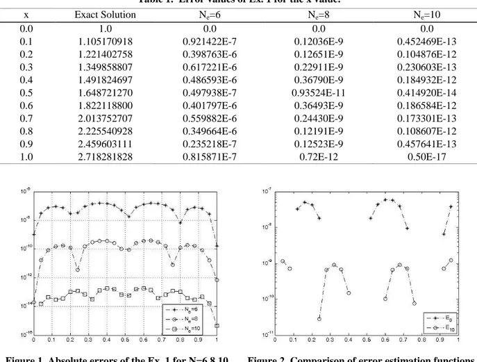
Obtained numerical values are reported in Table 1 (En10n). Moreover, in Fig.1, we compare the absolute errors for some values of N . These results are nearly equal to real values that show the high accuracy of the method. We plotted numerical results about error estimation functions for N 8,10 in Fig. 2.
Table 1. Error values of Ex. 1 for the x value.
Figure 1. Absolute errors of the Ex. 1 for N=6,8,10. Figure 2. Comparison of error estimation functions for N=8,10.
Example 2. Consider the following Fredholm-Volterra-integro differential equations
with the exact solution y(x)xex[33]:
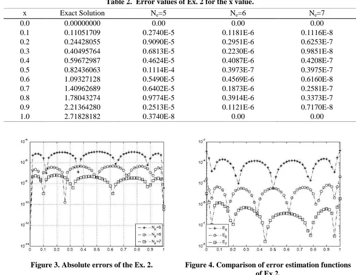
1 0 0 ) ( ) ( 2 2 ) ( ' x e y t dt y t dt y x x , y(0)0Table 2 and Figs. 3-4 show that numerical results and error respectively with the exact solution for various N .
x Exact Solution Ne=6 Ne=8 Ne=10
0.0 1.0 0.0 0.0 0.0
0.1 1.105170918 0.921422E-7 0.12036E-9 0.452469E-13
0.2 1.221402758 0.398763E-6 0.12651E-9 0.104876E-12
0.3 1.349858807 0.617221E-6 0.22911E-9 0.230603E-13
0.4 1.491824697 0.486593E-6 0.36790E-9 0.184932E-12
0.5 1.648721270 0.497938E-7 0.93524E-11 0.414920E-14
0.6 1.822118800 0.401797E-6 0.36493E-9 0.186584E-12
0.7 2.013752707 0.559882E-6 0.24430E-9 0.173301E-13
0.8 2.225540928 0.349664E-6 0.12191E-9 0.108607E-12
0.9 2.459603111 0.235218E-7 0.12523E-9 0.457641E-13
Table 2. Error values of Ex. 2 for the x value.
Figure 3. Absolute errors of the Ex. 2. Figure 4. Comparison of error estimation functions of Ex.2.
Example 3. Let us consider the following Volterra-integro differential equations with
the initial condition y(0)0[7]:
x x t y t dt x y 0 ) ( ' ) ( 4 1 ) ( ' , y(0)0The exact solution of this problem is sin(2 ) 2
1 )
(x x
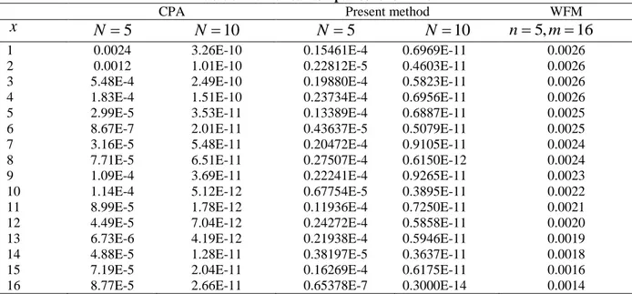
y . In Table 3, it has been given the comparison of absolute errors between the present method and Walsh function method (WFM), Chebyshev polynomial approach (CPA) for N 5, N 10 at
16
i
x . Given method absolutely arise that numerical results are better than other methods.
Example 4. Let us consider the following equation to compare present method and
Galerkin method [6]:
1 0 2 ln(1 ) 2 1 1 ) ( 1 2 ln 1 ) ( ) ( ' x x x dt t y t x x y x y , y(0)0 x Exact Solution Ne=5 Ne=6 Ne=7 0.0 0.00000000 0.00 0.00 0.000.1 0.11051709 0.2740E-5 0.1181E-6 0.1116E-8
0.2 0.24428055 0.9090E-5 0.2951E-6 0.6253E-7
0.3 0.40495764 0.6813E-5 0.2230E-6 0.9851E-8
0.4 0.59672987 0.4624E-5 0.4087E-6 0.4208E-7
0.5 0.82436063 0.1114E-4 0.3973E-7 0.3975E-7
0.6 1.09327128 0.5490E-5 0.4569E-6 0.6160E-8
0.7 1.40962689 0.6402E-5 0.1873E-6 0.2581E-7
0.8 1.78043274 0.9774E-5 0.3914E-6 0.3373E-7
0.9 2.21364280 0.2513E-5 0.1121E-6 0.7170E-8
In [6], Türkyılmazoğlu applied the Galerkin method with power series for this problem and obtained the following approximate solution:
10 9 8 7 6 5 4 3 2 10 001959235 . 0 01349909 . 0 04361917 . 09053189 . 0 1421647 . 0 1920182 . 0 248280 . 0 333105 . 0 4999834 . 0 9999995 . 0 ) ( x x x x x x x x x x x y
After the present method is applied, it is obtained the approximate solution:
10 9 8 7 6 5 4 3 2 10 0023408599 . 0 0155102920 . 0 048151052 . 0 096228429 . 0 14653433 . 0 19412019 . 0 2489071812 . 0 333215559 . 0 499999378 . 0 99999999 . 0 14 14 . 0 ) ( x x x x x x x x x x E x y
These numerical results are displayed in Fig.5. By aid of Fig.5, it is said that present method is better accurate than Galerkin method.
Table 3. Numerical comparisons for Ex.3.
CPA Present method WFM
x N 5 N 10 N 5 N 10 n5,m16
1 0.0024 3.26E-10 0.15461E-4 0.6969E-11 0.0026
2 0.0012 1.01E-10 0.22812E-5 0.4603E-11 0.0026
3 5.48E-4 2.49E-10 0.19880E-4 0.5823E-11 0.0026
4 1.83E-4 1.51E-10 0.23734E-4 0.6956E-11 0.0026
5 2.99E-5 3.53E-11 0.13389E-4 0.6887E-11 0.0025
6 8.67E-7 2.01E-11 0.43637E-5 0.5079E-11 0.0025
7 3.16E-5 5.48E-11 0.20472E-4 0.9105E-11 0.0024
8 7.71E-5 6.51E-11 0.27507E-4 0.6150E-12 0.0024
9 1.09E-4 3.69E-11 0.22241E-4 0.9265E-11 0.0023
10 1.14E-4 5.12E-12 0.67754E-5 0.3895E-11 0.0022
11 8.99E-5 1.78E-12 0.11936E-4 0.7250E-11 0.0021
12 4.49E-5 7.04E-12 0.24272E-4 0.5858E-11 0.0020
13 6.73E-6 4.19E-12 0.21938E-4 0.5946E-11 0.0019
14 4.88E-5 1.28E-11 0.38197E-5 0.3637E-11 0.0018
15 7.19E-5 2.04E-11 0.16269E-4 0.6175E-11 0.0016
16 8.77E-5 2.66E-11 0.65378E-7 0.3000E-14 0.0014
Example 5.
xy x y x x x y t dt xty t dt f x x y 0 1 0 ) ( ) ( ) ( ) cos( ) ( ) ( ' ) ( '' 1 ) 0 ( y , y'(0)y(0)0Consider the above Fredholm-Volterra integro differential equation. The exact solution of this problem y(x)sinxcosx, if we take
)) 1 cos( 2 ( ) cos sin 1 )( cos( ) cos sin ( ) (x x x x x x x x x f
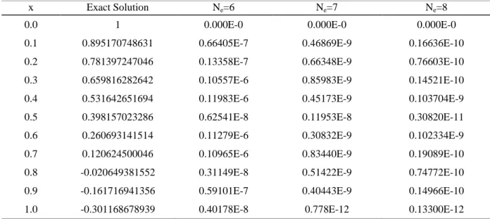
This problem has been solved by above numerical algorithm. Obtained numerical results are tabulated in Table 4. Absolute errors and error estimation functions are plotted in Figs. 6-7.
Table 4. Error values of Ex. 5 for the x value.
Figure 6. Absolute errors of the Ex. 5. Figure 7. Comparison of error estimation functions of Ex.5.
x Exact Solution Ne=6 Ne=7 Ne=8
0.0 1 0.000E-0 0.000E-0 0.000E-0
0.1 0.895170748631 0.66405E-7 0.46869E-9 0.16636E-10
0.2 0.781397247046 0.13358E-7 0.66348E-9 0.76603E-10
0.3 0.659816282642 0.10557E-6 0.85983E-9 0.14521E-10
0.4 0.531642651694 0.11983E-6 0.45173E-9 0.103704E-9
0.5 0.398157023286 0.62541E-8 0.11953E-8 0.30820E-11
0.6 0.260693141514 0.11279E-6 0.30832E-9 0.102334E-9
0.7 0.120624500046 0.10965E-6 0.83440E-9 0.19089E-10
0.8 -0.020649381552 0.31149E-8 0.51422E-9 0.74772E-10
0.9 -0.161716941356 0.59101E-7 0.40443E-9 0.14966E-10
Example 6. Let us consider the Fredholm integro differential equation [21]
1 0 2 1 2 ) ( ) 35 50 ( 1 1 ) ( 35 ) ( 50 ) ( '' x x e e y t dt x e x y x xy x y x x xt x 1 ) 0 ( y , y'(1)eExact solution of this problem is y(x)ex. The comparison of present method, Galerkin, Galerkin wavelet collocation method [20] is listed in Table 5 for N 6,7. Present method are more reliable than other methods from Table 5.
Table 5. Numerical comparisons for Ex.6. x
Present Method
6
N N7 Wavelet collocation[20] Wavelet Galerkin[20]
0.125 0.329E-7 0.256E-8 0.26E-3 0.27E-5
0.250 0.109E-7 0.132E-8 0.15E-3 0.30E-6
0.375 0.792E-7 0.156E-8 0.93E-4 0.26E-5
0.500 0.266E-7 0.254E-8 0.51E-4 0.43E-5
0.625 0.500E-7 0.421E-9 0.25E-4 0.56E-5
0.750 0.201E-7 0.922E-9 0.10E-4 0.65E-5
0.875 0.758E-7 0.312E-8 0.23E-5 0.72E-5
Example 7. Now, we take the following linear Volterra integro differential equation
with exact solution y(x)ex [34]:
1 0 ) ( cos 2 1 cos 2 1 ) ( ) ( ' ) ( '' x xy x xy x e x x xe y t dt y x t 1 ) 0 ( y , y'(0)1It has been given the comparison of the Present method and B-spline method [34] in Table 6. The given method is more accuracy than B-spline method for this problem.
Table 6. Numerical comparisons for Ex.7. x N8 Present Method N10 B-spline method [30] 10 1 h 20 1 h
0.0 0.100E-14 0.100E-16 0.13433E-13 0.149880E-13
0.1 0.56733E-10 0.379099E-11 0.702649E-9 0.444522E-10
0.2 0.132170E-9 0.194087E-10 0.290539E-8 0.183795E-9
0.3 0.48724E-10 0.613900E-11 0.675006E-8 0.425583E-9
0.4 0.145901E-9 0.239776E-10 0.123414E-7 0.776724E-9
0.5 0.86112E-10 0.329522E-11 0.197855E-7 0.124375E-8
0.6 0.96917E-10 0.231641E-10 0.291859E-7 0.183312E-8
0.7 0.80197E-10 0.441480E-12 0.406494E-7 0.217577E-8
0.8 0.53591E-10 0.163410E-10 0.542970E-7 0.340644E-8
0.9 0.11891E-10 0.456680E-11 0.702506E-7 0.440610E-8
Example 8. Consider the following Fredholm integro differential equation [5]:
1 0 2 / 1 ( ) ( ) ) ( ' y t dt f x t x t x y , y(0)0If y(x)x2(1x3 x2), which is the exact solution of this problem, the function f
can be calculated. For N 5, our method give us exact solution.
Example 9. Consider the Fredholm integro differential equation [5]:
1 0 3 / 1 ) ( ) ( ) ( ' x x t y t dt f x y , y(0)1Applying our method forN5,6, we get the approximate solution 1 ) 1 ( ) (x x5 xx2
y which is the exact solution. Here f can be calculated by Maple 13.
Example 10. Now, we give a nonlinear example in this problem. Let us consider the
following nonlinear Volterra integro differential equation [6, 35]:
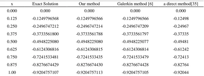
1 0 2 1 ) ( ) ( ' x y t dt y , y(0)0Numerical values of proposed method, Galerkin method [6] and a direct method [35] are showned in Table 7.
Table 7. Error values of Ex. 10 for the x value.
Example 11. Now, we consider the Volterra integro differential equation [4]:
) ( ) ( ) sin( ) ( 3 ) ( '' 0 x f dt t y t x x y x y x
, y(0) y'(1)0 where x x x x x x x x x xf( )23 3 2( 2 2)cos(2 )(2 1)sin(2 )sin 2cos
x Exact Solution Our method Galerkin method [6] a direct method[35]
0.000 0.000 0.000 0.000 0.000 0.125 -0.1249796568 -0.1249796566 -0.1249796566 -0.12498 0.250 -0.2496747212 -0.2496747214 -0.2496747209 -0.24967 0.375 -0.3733561800 -0.3733561788 -0.3733561797 -0.37335 0.500 -0.4948225080 -0.4948225080 -0.4948225077 -0.49481 0.625 -0.6124306816 -0.6124306815 -0.6124306814 -0.61242 0.750 -0.7241533481 -0.7241533435 -0.7241533479 -0.72413 0.875 -0.8276674429 -0.8276674430 -0.8276674428 -0.82764 1.00 -0.9204757107 -0.9204757113 -0.9204757105 -0.92044
The approximate solution generated by the proposed method is x2 x which is the exact solution of this problem.
Example 12. Consider the FVIDE
x dt t y t x dt t y t x x x x x x y x xy x xy 0 1 0 2 3 4 ) ( ) ( ) ( ) ( 12 17 6 13 2 1 6 1 12 1 ) ( 2 ) ( ' ) ( ''subject to initial conditions y(0)1, y'(0)2y(1)2y(0)1. For N 2,3,4,5, we obtain 1
)
(x x2 x
y which is the exact solution.
Example 13. Consider the nonlinear Volterra integro differential equation [11]:
x y t y t dt x y 0 1 ) ( ' ) ( ) ( ' , y(0)0The exact solution is y(x) 2tan(x/ 2). In [11], it has been solved by Haar wavelets collocation method. Maximum absolute errors around 103 in [11] from N5 to
35
N . Our method is presented more accuracy values from Table 8. Table 8. Error values of Ex. 13 for the x value.
3.2. DISCUSSION
The effectiveness of the method is examined by comparing the obtained results with the exact solutions and other methods. The proposed method presents us more convenient numerical results than compared methods in Ex. 3, 5-7, 13. A useful feature of this method is to find the analytical solutions if the problem has exact solutions that are polynomial functions in Ex. 8, 9, 11 and 12. The advantage of the method over others is that only small size operational matrix is required to provide the solution of high accuracy because most of matrix involves more numbers of zeroes and thus, reduces the run time. Also, the absolute error may be decreased if we take more Chebyshev terms. Even if the numerical algorithm is introduced linear FVIDs, some nonlinear examples are presented in Ex.10 and 13. It is easy to write PC codes which are related to obtained system for necessary computation in Maple 13. Moreover, the graphs are genarate by aid of Matlab 2007.
x Exact Solution Ne 6 Ne 8 Ne 10
0.0 0.0 0.55000E-15 0.18100E-15 0.0E-0
0.2 0.2013440870 0.452076E-5 0.719203E-7 0.122421E-8
0.4 0.4110194227 0.583033E-5 0.119630E-6 0.122421E-8
0.6 0.6387957040 0.554064E-5 0.130914E-6 0.264398E-8
0.8 0.8978815369 0.430861E-5 0.104877E-6 0.794482E-9
4. CONCLUSION
In this paper, we used the operational matrix method with Chebyshev polynomials to obtain numerical solutions of the FVID equations. The properties of the Chebyshev operational matrix method is utilized to reduce the problem to solving the system of nonlinear algebraic equations with unknown coefficients.
REFERENCES
[1] Delves L.M., Mohamed J.L., Computational Methods for Integral Equations, Cambridge University Press, Cambridge, 1985.
[2] Wazwaz A.M., A First Course in Integral Equations, World Scientifics, Singapore, 1997.
[3] Huang Y., Li X.F., International J. of Computer Mathematics, 87(6), 1288, 2010.
[4] Kashkaria B.S.H., Syam M.I., Journal of Computational and Applied Mathematics, 311, 314, 2017.
[5] Turkyılmazoğlu M., Applied Mathematics and Computation, 247, 410, 2014. [6] Turkyilmazoglu M., Applied Mathematics and Computation, 227, 384, 2014. [7] Akyüz-Daşçıoğlu A., Applied Mathematics and Computation 181, 103, 2006. [8] Gülsu M., Öztürk Y., Applied Mathematics and Computation 216, 2183, 2010.
[9] Tavassoli KajaniM., Ghasemi M, Babolian E., Applied Mathematics and Computation,
180, 569, 2006.
[10] Sezer M., Gülsu M., Applied Mathematics and Computations, 185, 6465, 2007.
[11] Islam S., Aziz I., Feyyaz M., International J. of Computer Mathematics, 90(9), 1971, 2013.
[12] Bhrawy A.H., Tohidi E., Soleymani F., Applied Mathematics and Computations, 219, 482, 2012
.
[13] Noor M., Mohyud-Din S., Applied Mathematics and Computations, 3(6), 188, 2008. [14] Gachpazan M., Kerayechian A., Zeidabadi H., J. Inform. Comput. Sci., 9(4), 289, 2014. [15] Maleknejad K., Attary M, Commun. Nonlinear Sci. Numer. Simul., 16, 2672, 2011. [16] Wazwaz A., Rach R., Duan J., Appl. Math. Comput., 219(10), 5004, 2013.
[17] Shahmorad S., Applied Mathematics and Computations, 167, 1418, 2005.
[18] Parvaz R., Zarebnia M., Bagherzadeh A.S., Mathematical Modelling and Analysis, 21 (6), 719, 2016.
[19] Dehghan M., Saadatmandi A., International Journal of Computer Mathematics, 85 (1) 123, 2008.
[20] Body J.P., Chebyshev and Fourier Spectral methods, University of Michigan, New York 2000.
[21] Maleknejad K., Sohrabi S., Derili H., International Journal of Computer Mathematics,
87 (2), 327, 2010.
[22] Momani S., Noor M.A., Appl. Math. Comp., 182, 754, 2006. [23] Vanani S.K., Aminataei A., Comp. Appl. Math., 30 (3), 655, 2011.
[24] Öztürk Y., Gülsu M., Mathematical Methods in Applied Sciences, 37, 2227,2014. [25] Babolian E., Fattahzadeh F., Appl. Math. Comp., 188, 417, 2007.
[26] Saadatmandi A., Dehghan M., Comp. Math. Appl., 59, 1326, 2010. [27] Aznam S.M., Chowdhury M.S.H., Results in Physics, 11, 243,
[28] Hesameddini E., Shahbazi M., Applied Mathematics and Computation, 322, 40, 2018. [29] Rani D., Mishra V., Results in Physics, 16, 102836, 2020.
[30] Pourbabaee M., Saadatmandi A., Applied Mathematics and Computation, 361, 215, 2019.
[31] Kreyszig E., Introductory Functional Analysis with Applications, John Wiley and sons. Inc., 1978.
[32] Mason J.C., Handscomb D.C., Chebyshev Polynomials, Chapman and Hall/CRC, New York, 2003.
[33] Shahooth M.K., Ahmad R.R., Din K.S., Swidan W., Al-Husseini O.K., Shahooth W.K., J. Appl. Computant Math, 5, 298, 2016.
[34] Mahmoodi Z., Rashidinia J, Babolian E., Applicable Analysis An International Journal
92(9), 1787, 2013.
copyright holder's express written permission. However, users may print, download, or email articles for individual use.
![Table 6. Numerical comparisons for Ex.7. x N 8 Present Method N 10 B-spline method [30] 101h 201h](https://thumb-eu.123doks.com/thumbv2/9libnet/3843986.34291/14.892.96.794.828.1139/table-numerical-comparisons-ex-present-method-spline-method.webp)