Dergi web sayfası:
www.agri.ankara.edu.tr/dergi www.agri.ankara.edu.tr/journalJournal homepage:
TARIM BİLİMLERİ DERGİSİ
—
JOURNAL OF AGRICUL
TURAL SCIENCES
22 (2016) 32-41
Identifying Irregular Potatoes by Developing an Intelligent Algorithm
Based on Image Processing
Afshin AZIZIa, Yousef ABBASPOUR-GILANDEHa
aUniversity of Mohagheghe Ardabili, Faculty of Agricultural Technology and Natural Resources, Department of Mechanics of Agricultural
Machinery, Ardabil, IRAN
ARTICLE INFO
Research Article
Corresponding Author: Yousef ABBASPOUR-GILANDEH, E-mail: [email protected], Tel: +98 (914) 451 62 55 Received: 13 September 2014, Received in Revised Form: 27 November 2014, Accepted: 01 December 2014
ABSTRACT
The objective of this study was to develop an algorithm based on image processing for detecting misshapen potatoes from the mass of potatoes and obtaining homogeneous products. The database used in this research included the digital images acquired from Agria variety of Ardabil (Iranian northern-west) potato with different sizes and shapes. A combination of morphological features including geometrical features like length, width and features related to shape such as roundness were taken into consideration in identifying irregular potatoes from others employing elongation and Fourier descriptors. Using statistical principal component analysis (PCA), seven features were selected as the most prominent for classification. The experimental results showed that the proposed method achieves a high level of accuracy with merely seven selected discriminative features, obtaining an average correct classification rate of 98% for training set. Additionally, regular potatoes were separated into small, medium and large categories with 100% accuracy. According to the results, the developed algorithm based on image processing can be used in classifying products with no proper shape.
Keywords: Classification; Image processing; Irregularity; Potato; Shape
Görüntü İşleme Tabanlı Akıllı Algoritma Geliştirerek Şekilsiz
Patateslerin Belirlenmesi
ESER BİLGİSİ
Araştırma Makalesi
Sorumlu Yazar: Yousef ABBASPOUR-GILANDEH, E-posta: [email protected], Tel: +98 (914) 451 62 55 Geliş Tarihi: 13 Eylül 2014, Düzeltmelerin Gelişi: 27 Kasım 2014, Kabul: 01 Aralık 2014
ÖZET
Bu çalışmanın amacı görüntü işleme tabanlı akıllı algoritma geliştirerek şekilsiz patateslerin belirlenmesi ve homojen şekilli patates elde edilmesidir. Materyal olarak İran’ın kuzeybatısında bulunan Ardabil bölgesinin Agria patates çeşidinin farklı boyut ve farklı görüntüleri kullanılmıştır. Şekilsiz patateslerin belirlenmesinde uzunluk, genişlik, yuvarlaklık gibi farklı özellikler göz önüne alınmış ve uzama ile Fourier tanımlayıcılarından yararlanılmıştır. İstatistik analize (PCA)
Identifying Irregular Potatoes by Developing an Intelligent Algorithm Based on Image Processing, Azizi & Abbaspour-Gilandeh
1. Introduction
After wheat, maize, and rice, potato is the fourth most produced food in the world. Moreover, with over 4 million tons of potatoes Iran is ranked eighth in the world and third in Asia after China and India in terms of producing potato (FAO 2011). The high variety in size and shape along with damage-vulnerability has turned potato into a difficult crop as far as handling and grading. As a part of food industry the appearance and shape of the product play a significant role. This issue is particularly important concerning potatoes because the misshapen tubers have a lot of losses during peeling and subsequent processing such as cutting and drying. From of the view of a consumer, a good product is that which has a proper shape and appearance. Moreover, customers and food inspectors prefer regular potatoes. Hence, to achieve a homogeneous product, identifying and separating irregular potatoes is required in food production chain.
For reasons such as inconsistency, subjectivity and variability of potato sorting by workers, manual processes are, more often than not, considered extremely harsh and easily affected by environmental conditions such as changes in temperature and moisture (Razmjooy et al 2012). Often, separation and classification of misshapen potatoes from sound tubers is done by workers based on their indigenous knowledge, a fact which increases labor cost as well as human errors and production losses (Zhou et al 1998). In developed countries, such artificial intelligences as machine vision, with their many benefits, are widely used in the inspection of agri-production (Moreda et al 2012).
Advantages such as high accuracy, high speed, relatively low cost and repeatability have led
most modern manufactures to utilize machine vision systems. In other words, in order to have a better quality control in food industry, machine vision technique has replaced other methods (Cubero et al 2011). Regarding the application of these systems in controlling and monitoring agricultural productions, numerous studies have been conducted (Aleixos et al 2002; Choudhary et al 2008; Al-Mallahi et al 2010; Barnes et al 2010; Liming & Yanchao 2010; Arribas et al 2011; Li et al 2012; Nashat et al 2014).
Determining shape is one of the most common processes of food quality assessment (Du & Sun 2004). It should be noted that shape is a major problem in potato inspection as potato tubers have various shapes affected by the environment resulting in irregularities. Incoming damage to the tuber during harvesting and transportation causes the formation of different shapes. Potato tubers are normally spherical or rectangular with smooth surface while those with more outgrowth and dip are considered to be misshapen. The shape can be analyzed through such different methods as invariant moments, boundary encoding, bending energy, fractals and Fourier description among which invariant moments and Fourier description are most commonly used owing to the fact that they are not dependent on scale and orientation.
As a result of the aforementioned points and also the need for sorting out units and food factories in Iran, particularly concerning potato production, the aim of this research was to separate irregular potatoes from other tubers and grade well-shaped (regular) potatoes in various categories based on their size and manner of offline machine vision. dayalı olarak sınıflandırmada çok önemli olan 7 özellik seçilmiştir. Araştırma sonucunda önerilen 7 yöntemin yüksek bir doğruluğa sahip olduğu, sınıflandırmada ortalama % 98 doğruluk oranına ulaştığı görülmüştür. Ayrıca patatesler % 100 oranında küçük, orta ve büyük gruplara ayrılabilmiştir. Elde edilen sonuçlara göre geliştirilen görüntü işleme tabanlı algoritma şekilsiz ürünlerin sınıflandırılmasında kullanılabilir.
Anahtar Kelimeler: Sınıflandırma; Görüntü işleme; Şekil bozukluğu; Patates; Biçim
2. Material and Methods
2.1. Preparing potato samples
A set of potato tubers of Agria variety (as a common variety) related to 2012 harvest was randomly collected from Ardabil (Iranian northern-west) Central Agricultural Research Center in different sizes and shapes. The tubers were removed from adherent clods and other waste materials during harvesting, carrying, and packaging so that all the samples had relative cleanliness. For the final evaluation, potatoes were primarily classified manually into well-shaped and misshapen with relative irregularity as the criterion. Figure 1 shows some of these regular and irregular potatoes. For the ‘train and test’ method, the available data is generally divided into two parts:training set and test set (Bramer 2007). First, the training set is used to construct a classifier (decision tree, neural net etc.). The classifier is then used to predict the classification for the instances in the test set. Accordingly, the database was divided into two parts, a training set and a test set, where the former was composed of 252 potatoes with 210 voted as regular and 42 as irregular (small, medium and large sizes). The testing set included 202 tubers with 178 regular and 24 irregular potato tubers so as to validate the prediction model in an offline mode. The aim of set was to evaluate and prepare the system for real-time applications.
Figure 1- Examples of the database images: a, regular potatoes, and b, irregular potatoes
Şekil 1- Görüntü örnekleri: a, şekli düzgün patatesler; b, şekli bozuk patatesler
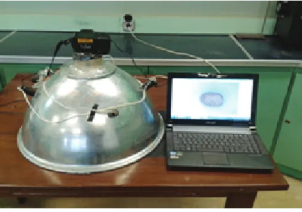
2.2. Image acquisition system
Image acquisition system shown in Figure 2 is a dome-shaped chamber, in which LED light bulbs and fluorescent are used to supply the lighting conditions. The lighting chamber is made of a stainless steel sheet. Lighting is an important and effective factor as far as image quality is concerned since lighting method and light source influence subsequent process and the obtained results. Hence, the LED bulbs were located at an angle of 45 degrees from the potatoes as there was no shadow around samples in this angle. Therefore, in order to eliminate shade and other undesired information, direct radiation was not used. The camera used in this research was a CCD camera (SONY ∝200) with the resolution of 10.1 mega pixel and 40 mm close-up lens with focal a length of 70 mm and aperture setting of F5.6. Such a well-chosen lighting system allowed the potatoes to be properly recognized and analyzed in the images. Therefore, there was no need for extra image processing. Due to the light reflection lake, Steinbach white paper was employed as background. The main advantage of this type of paper is light absorption rather than reflection. Digital images were taken with the resolution of 3872x2592 pixels under the same lighting condition and 12 VDC; next, they were transferred to the hard disc of a computer via USB
Figure 2- Image acquisition system
Identifying Irregular Potatoes by Developing an Intelligent Algorithm Based on Image Processing, Azizi & Abbaspour-Gilandeh
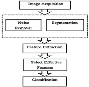
cable. Because of the CPU limitations, the images were converted into 968×648 resolution by resize operator. The images were processed and analyzed using the image processing toolbox of MATLAB R2012 software. The process of identifying irregular potatoes is shown in the flowchart of Figure 3.
Figure 3- Flowchart of the image processing algorithm for discriminating irregular potatoes
Şekil 3- Şekli bozuk patateslerin belirlenmesinde kullanılan görüntü işleme algoritmasının akış diyagramı
2.3. Image pre-processing and segmentation
Although our image acquisition camera produced high contrast images, a pre-processing was needed in order to extract the usable features of each image for the analysis of the potato shape. This pre-processing included noise and background removal from the potato image in which they have redundant information. If noise and other undesired information were not removed, the image analysis would face different problems which would ultimately make it harder to obtain homogeneity. In other words, most of
the subsequent processing such as image filtering, boundary detection, segmentation and feature extraction would fail to accurately determine the objects real boundaries due to the non-uniform illumination and noise in the image background. Hence, correcting non uniform illumination in the background can be useful in this regard. A linear Gaussian low pass filter (Castleman 1996) and morphological operations such as opening were used to reduce the noise and obtain images with a uniform background.
Image segmentation is the process of partitioning a digital image into multiple segments (set of pixels). In other words, in segmentation, pixels are clustered into salient image regions (i.e., regions corresponding to individual surfaces, objects, or natural parts of objects). The goal of segmentation is to simplify and/or change the representation of an image into something that is more meaningful and easier to analyze (Shapiro & Stockman 2001). The color of potatoe arils varies from yellow to red, corresponding to high R values. Hence, the segmentation used a pre-defined threshold in the R band. In fact, segmentation was approached by attempting to find the boundaries between regions and use global thresholding in the red ban. The pixels lower than this value belonged to the background (displayed in black pixels) and higher pixels were considered as foreground (the object displayed in white pixels). Since the intensity distributions of potatoes and background pixels were sufficiently distinct (after noise removal), it was possible to use a single (global) threshold applicable over the entire images. Thus, the algorithm was able to automatically estimate the required threshold value for each image. The results of pre-processing and segmentation and also the boundary or contour image of a potato are shown in Figure 4. It should be noted that both noise removal and segmentation processes did not take place simultaneously, rather in a tandem at a specific stage titled pre-processing.
Görüntü İşleme Tabanlı Akıllı Algoritma Geliştirerek Şekilsiz Patateslerin Belirlenmesi, Azizi & Abbaspour-Gilandeh
Figure 4- Results of pre-processing and segmentation operations: a, original image; b, uniformed background; c, segmented image; d, boundary of potato
Şekil 4- Ön işleme ve dilimleme işlem sonuçları: a, original görüntü; b, uniform olmayan arka görüntü; c, dilimlenmiş görüntü; d, patates görüntü çizgisi
2.4. Extracting morphological features 2.4.1. Calculating geometrical characteristics
Extracting different features is a major stage after pre-processing. Certain geometrical features such as perimeter, area, length and width were calculated from the binary images. For instance, the perimeter can be measured by tracing the boundary of the potato and summing all the steps of length 1 or
4
segmentation and feature extraction would fail to accurately determine the objects real boundaries due to the non-uniform illumination and noise in the image background. Hence, correcting non non-uniform illumination in the background can be useful in this regard. A linear Gaussian low pass filter (Castleman 1996) and morphological operations such as opening were used to reduce the noise and obtain images with a uniform background.
Image segmentation is the process of partitioning a digital image into multiple segments (set of pixels). In other words, in segmentation, pixels are clustered into salient image regions (i.e., regions corresponding to individual surfaces, objects, or natural parts of objects). The goal of segmentation is to simplify and/or change the representation of an image into something that is more meaningful and easier to analyze (Shapiro & Stockman 2001). The color of potatoe arils varies from yellow to red, corresponding to high R values. Hence, the segmentation used a pre-defined threshold in the R band. In fact, segmentation was approached by attempting to find the boundaries between regions and use global thresholding in the red ban. The pixels lower than this value belonged to the background (displayed in black pixels) and higher pixels were considered as foreground (the object displayed in white pixels). Since the intensity distributions of potatoes and background pixels were sufficiently distinct (after noise removal), it was possible to use a single (global) threshold applicable over the entire images. Thus, the algorithm was able to automatically estimate the required threshold value for each image. The results of pre-processing and segmentation and also the boundary or contour image of a potato are shown in Figure 4. It should be noted that both noise removal and segmentation processes did not take place simultaneously, rather in a tandem at a specific stage titled pre-processing.
Figure 4- Results of pre-processing and segmentation operations: a, original image; b, uniformed background; c, segmented image; d, boundary of potato
Şekil 4- Ön işleme ve dilimleme işlem sonucuçları: a, original görüntü; b, uniform olmayan arka görüntü; c, dilimlenmiş görüntü; d, patates görüntü çizgisi
2.4. Extracting morphological features 2.4.1. Calculating geometrical characteristics
Extracting different features is a major stage after pre-processing. Certain geometrical features such as perimeter, area, length and width were calculated from the binary images. For instance, the perimeter can be measured by tracing the boundary of the potato and summing all the steps of length 1 or √2 taken from Figure 4d. In fact, length 1 is the distance between two adjacent pixels and √2 is the distance at the corners of the boundary in rectangular shapes. The area equaled the total number of white pixels in the binary image. For length and width we computed the Euclidean distance transform of the binary image. In fact for each pixel in the binary image, the distance transform is assigned a number that is the distance between that pixel and the nearest nonzero pixel of binary image shown in Figure 5. In the
two-dimensional area, the Euclidean distance between (𝑥𝑥𝑥𝑥1, 𝑦𝑦𝑦𝑦1) and (𝑥𝑥𝑥𝑥2, 𝑦𝑦𝑦𝑦2) was calculated by the Equation 1 (Gonzalez
& Woods 2008). Moreover, through combining geometrical characteristics, several features were obtained such as elongation, roundness, extent and eccentricity which formulation exist in the appendix.
�(𝑥𝑥𝑥𝑥1− 𝑥𝑥𝑥𝑥2)2+ (𝑦𝑦𝑦𝑦1− 𝑦𝑦𝑦𝑦2)2 (1)
taken from Figure 4d. In fact, length 1 is the distance between two adjacent pixels and
segmentation and feature extraction would fail to accurately determine the objects real boundaries due to the non-uniform illumination and noise in the image background. Hence, correcting non non-uniform illumination in the background can be useful in this regard. A linear Gaussian low pass filter (Castleman 1996) and morphological operations such as opening were used to reduce the noise and obtain images with a uniform background.
Image segmentation is the process of partitioning a digital image into multiple segments (set of pixels). In other words, in segmentation, pixels are clustered into salient image regions (i.e., regions corresponding to individual surfaces, objects, or natural parts of objects). The goal of segmentation is to simplify and/or change the representation of an image into something that is more meaningful and easier to analyze (Shapiro & Stockman 2001). The color of potatoe arils varies from yellow to red, corresponding to high R values. Hence, the segmentation used a pre-defined threshold in the R band. In fact, segmentation was approached by attempting to find the boundaries between regions and use global thresholding in the red ban. The pixels lower than this value belonged to the background (displayed in black pixels) and higher pixels were considered as foreground (the object displayed in white pixels). Since the intensity distributions of potatoes and background pixels were sufficiently distinct (after noise removal), it was possible to use a single (global) threshold applicable over the entire images. Thus, the algorithm was able to automatically estimate the required threshold value for each image. The results of pre-processing and segmentation and also the boundary or contour image of a potato are shown in Figure 4. It should be noted that both noise removal and segmentation processes did not take place simultaneously, rather in a tandem at a specific stage titled pre-processing.
Figure 4- Results of pre-processing and segmentation operations: a, original image; b, uniformed background; c, segmented image; d, boundary of potato
Şekil 4- Ön işleme ve dilimleme işlem sonucuçları: a, original görüntü; b, uniform olmayan arka görüntü; c, dilimlenmiş görüntü; d, patates görüntü çizgisi
2.4. Extracting morphological features 2.4.1. Calculating geometrical characteristics
Extracting different features is a major stage after pre-processing. Certain geometrical features such as perimeter, area, length and width were calculated from the binary images. For instance, the perimeter can be measured by tracing the boundary of the potato and summing all the steps of length 1 or √2 taken from Figure 4d. In fact, length 1 is the distance between two adjacent pixels and √2 is the distance at the corners of the boundary in rectangular shapes. The area equaled the total number of white pixels in the binary image. For length and width we computed the Euclidean distance transform of the binary image. In fact for each pixel in the binary image, the distance transform is assigned a number that is the distance between that pixel and the nearest nonzero pixel of binary image shown in Figure 5. In the
two-dimensional area, the Euclidean distance between (𝑥𝑥𝑥𝑥1, 𝑦𝑦𝑦𝑦1) and (𝑥𝑥𝑥𝑥2, 𝑦𝑦𝑦𝑦2) was calculated by the Equation 1 (Gonzalez
& Woods 2008). Moreover, through combining geometrical characteristics, several features were obtained such as elongation, roundness, extent and eccentricity which formulation exist in the appendix.
�(𝑥𝑥𝑥𝑥1− 𝑥𝑥𝑥𝑥2)2+ (𝑦𝑦𝑦𝑦1− 𝑦𝑦𝑦𝑦2)2 (1)
is the distance at the corners of the boundary in rectangular shapes. The area equaled the total number of white pixels in the binary image. For length and width we computed the Euclidean distance transform of the binary image. In fact for each pixel in the binary image, the distance transform is assigned a number that is the distance between that pixel and the nearest nonzero pixel of binary image shown in Figure 5. In the two-dimensional area, the Euclidean distance between (x1, y1) and (x2, y2) was calculated by the Equation 1 (Gonzalez & Woods 2008). Moreover, through combining geometrical characteristics, several features were obtained such as elongation,
roundness, extent and eccentricity which equation exist in the appendix.
4
can be useful in this regard. A linear Gaussian low pass filter (Castleman 1996) and morphological operations such as opening were used to reduce the noise and obtain images with a uniform background.
Image segmentation is the process of partitioning a digital image into multiple segments (set of pixels). In other words, in segmentation, pixels are clustered into salient image regions (i.e., regions corresponding to individual surfaces, objects, or natural parts of objects). The goal of segmentation is to simplify and/or change the representation of an image into something that is more meaningful and easier to analyze (Shapiro & Stockman 2001). The color of potatoe arils varies from yellow to red, corresponding to high R values. Hence, the segmentation used a pre-defined threshold in the R band. In fact, segmentation was approached by attempting to find the boundaries between regions and use global thresholding in the red ban. The pixels lower than this value belonged to the background (displayed in black pixels) and higher pixels were considered as foreground (the object displayed in white pixels). Since the intensity distributions of potatoes and background pixels were sufficiently distinct (after noise removal), it was possible to use a single (global) threshold applicable over the entire images. Thus, the algorithm was able to automatically estimate the required threshold value for each image. The results of pre-processing and segmentation and also the boundary or contour image of a potato are shown in Figure 4. It should be noted that both noise removal and segmentation processes did not take place simultaneously, rather in a tandem at a specific stage titled pre-processing.
Figure 4- Results of pre-processing and segmentation operations: a, original image; b, uniformed background; c, segmented image; d, boundary of potato
Şekil 4- Ön işleme ve dilimleme işlem sonucuçları: a, original görüntü; b, uniform olmayan arka görüntü; c, dilimlenmiş görüntü; d, patates görüntü çizgisi
2.4. Extracting morphological features 2.4.1. Calculating geometrical characteristics
Extracting different features is a major stage after pre-processing. Certain geometrical features such as perimeter, area, length and width were calculated from the binary images. For instance, the perimeter can be measured by tracing the boundary of the potato and summing all the steps of length 1 or √2 taken from Figure 4d. In fact, length 1 is the distance between two adjacent pixels and √2 is the distance at the corners of the boundary in rectangular shapes. The area equaled the total number of white pixels in the binary image. For length and width we computed the Euclidean distance transform of the binary image. In fact for each pixel in the binary image, the distance transform is assigned a number that is the distance between that pixel and the nearest nonzero pixel of binary image shown in Figure 5. In the
two-dimensional area, the Euclidean distance between (𝑥𝑥𝑥𝑥1, 𝑦𝑦𝑦𝑦1) and (𝑥𝑥𝑥𝑥2, 𝑦𝑦𝑦𝑦2) was calculated by the Equation 1 (Gonzalez
& Woods 2008). Moreover, through combining geometrical characteristics, several features were obtained such as elongation, roundness, extent and eccentricity which formulation exist in the appendix.
�(𝑥𝑥𝑥𝑥1− 𝑥𝑥𝑥𝑥2)2+ (𝑦𝑦𝑦𝑦1− 𝑦𝑦𝑦𝑦2)2 (1) (1)
Figure 5- Length and width of a sample potato extracted from binary image
Şekil 5- İkili görüntüden elde edilen örnek patatesin uzunluğu ve genişliği
2.4.2. Extracting fourier descriptors
Describing the shapes of crops, while often simple and easy for human eyes and brains, is difficult for a computer. In other words, computer descriptors are deterministic and quantitative yet, they are subjective forman (Ying et al 2002). A 1-D functional representation of a boundary namely signature was employed. Regardless of how a signature is generated, however, the basic idea is to reduce the boundary representation to a 1-D function which is presumably easier to describe than the original 2-D boundary (Gonzalez & Woods 2008). Thus, as shown in figure 6 the radius signature r(k) was obtained from potato boundaries and the starting point in the contour was determined at the minimum distance of r(k) on clockwise. As mentioned in the previous section, Fourier descriptor is a common and reliable technique for the analysis of agri-productions shapes. Hence, after obtaining the radius signature, it was transferred into Fourier domain in order for coefficients to be calculated as Fourier descriptors of the boundary.
Identifying Irregular Potatoes by Developing an Intelligent Algorithm Based on Image Processing, Azizi & Abbaspour-Gilandeh
37
Ta r ı m B i l i m l e r i D e r g i s i – J o u r n a l o f A g r i c u l t u r a l S c i e n c e s 22 (2016) 32-41Figure 6- a, external boundary of a potato with its centroid point; b, corresponding boundary signature
Şekil 6- a, merkezinden itibaren bir patatesin dış sınırları; b, ilgili sınır işaretleri
In order to analyze the potato shapes, fast Fourier transform of r(k) was calculated using Equation (2) (Gonzalez & Woods 2008):
5
Figure 5- Length and width of a sample potato extracted from binary image
Şekil 5- İkili görüntüden elde edilen örnek patatesin uzunluğu ve genişliği 2.4.2. Extracting fourier descriptors
Describing the shapes of crops, while often simple and easy for human eyes and brains, is difficult for a computer. In other words, computer descriptors are deterministic and quantitative yet, they are subjective forman (Ying et al 2002). A 1-D functional representation of a boundary namely signature was employed. Regardless of how a signature is generated, however, the basic idea is to reduce the boundary representation to a 1-D function which is presumably easier to describe than the original 2-D boundary (Gonzalez & Woods 2008). Thus, as shown in figure 6 the radius signature r(k) was obtained from potato boundaries and the starting point in the contour was determined at the minimum distance of r(k) on clockwise. As mentioned in the previous section, Fourier descriptor is a common and reliable technique for the analysis of agri-productions shapes. Hence, after obtaining the radius signature, it was transferred into Fourier domain in order for coefficients to be calculated as Fourier descriptors of the boundary.
Figure 6- a, external boundary of a potato with its centroid point; b, corresponding boundary signature
Şekil 6- a, merkezinden itibaren bir patatesin dış sınırları; b, ilgili sınır işaretleri
In order to analyze the potato shapes, fast Fourier transform of r(k) was calculated using Equation (2) (Gonzalez & Woods 2008):
𝐹𝐹𝐹𝐹(ℎ) =𝑁𝑁𝑁𝑁 � 𝑟𝑟𝑟𝑟1 (𝑘𝑘𝑘𝑘)𝑒𝑒𝑒𝑒−𝑗𝑗𝑗𝑗2𝜋𝜋𝜋𝜋ℎ𝑘𝑘𝑘𝑘�𝑁𝑁𝑁𝑁 ℎ = 0,1,2, … , 𝑁𝑁𝑁𝑁 − 1
𝑁𝑁𝑁𝑁 𝑘𝑘𝑘𝑘=1
(2) Where; N is the number of pixels in the boundary. The inverse Fourier transform of these coefficients restores r(k) that is, from Equation (3) (Gonzalez & Woods 2008):
(2) Where; N is the number of pixels in the boundary. The inverse Fourier transform of these coefficients restores r(k) that is, from Equation (3) (Gonzalez & Woods 2008):
6
𝑟𝑟𝑟𝑟(𝑘𝑘𝑘𝑘) =𝑁𝑁𝑁𝑁 � 𝐹𝐹𝐹𝐹1 (ℎ). 𝑒𝑒𝑒𝑒𝑗𝑗𝑗𝑗2𝜋𝜋𝜋𝜋ℎ𝑘𝑘𝑘𝑘�𝑁𝑁𝑁𝑁 𝑁𝑁𝑁𝑁 ℎ=1 (3) We know from discussions of the Fourier transform that instead of all the Fourier coefficients, only the first P coefficients are employed. This is equivalent to setting 𝐹𝐹𝐹𝐹(ℎ)= 0 for ℎ > 𝑃𝑃𝑃𝑃 − 1 in Equation (3). The result is the following approximation to r(k) (Gonzalez & Woods 2008):𝑟𝑟𝑟𝑟̂(𝑘𝑘𝑘𝑘) =𝑃𝑃𝑃𝑃 � 𝐹𝐹𝐹𝐹(ℎ)𝑒𝑒𝑒𝑒1 𝑗𝑗𝑗𝑗2𝜋𝜋𝜋𝜋ℎ𝑘𝑘𝑘𝑘�𝑃𝑃𝑃𝑃 𝑃𝑃𝑃𝑃
ℎ=1
(4) Although only P terms were used to obtain each 𝑟𝑟𝑟𝑟̂(𝑘𝑘𝑘𝑘), k still ranges from 1 to 𝑁𝑁𝑁𝑁 − 1. That is meaning the same number of points exists in the approximate boundary, but not as many terms were used in the reconstruction of each point (Gonzalez & Woods 2008). In this research, P was 10 meaning that the first 10 harmonics could describe the shape of potato tubers. Figure 7(b) shows the boundary of an irregular potato, consisting of 2384 points. The corresponding 2384 Fourier descriptors were obtained for this boundary using Equation (2). The objective of this illustration was to examine effects of reconstructing the boundary based on decreasing the number of Fourier descriptors (Gonzalez & Woods 2008).
Figure 7- a, color segmented image of an irregular potato; b, boundary of potato tuber (2384 points); c-f, boundaries reconstructed using 72, 36, 18, and 8 Fourier descriptors, respectively. These points are approximately 3%, 1.5%, 0.75%, and 0.34% of 2384, respectively
Şekil 7- a, şekilsiz patatesin renk dilimli görüntüsü; b, 2384 noktadaki patates sınırı; c-f, 8, 18, 36 ve 72 Forier tanımlayıcıları kullanarak yeniden yapılan sınırlardır. Bu noktalar sırasıyla 2384 noktanın yaklaşık olarak % 3, % 1.5, % 0.75 ve % 0.34’dür
The changes in the frequency of Potato boundary can be represented by the harmonic components (𝐹𝐹𝐹𝐹(ℎ)) in the Fourier domain. For instance, 𝐹𝐹𝐹𝐹(0) is the average radius, 𝐹𝐹𝐹𝐹(1) represents the bending of an object, and 𝐹𝐹𝐹𝐹(2) shows the elongation of the object and so on. Interpretation of the first few Fourier coefficients of radius boundary is summarized in Table 1.
Table 1- Shape extraction from radius boundary Fourier coefficients
Çizelge 1-Yarıçap sınır Fourier katsayılarından şekil çıkarma
Fourier coefficient Implied shape information
𝐹𝐹𝐹𝐹(0) Average radius
𝐹𝐹𝐹𝐹(1) Bending
𝐹𝐹𝐹𝐹(2) Elongation
𝐹𝐹𝐹𝐹(3) Triangle
𝐹𝐹𝐹𝐹(4) Square
A regular round potato has a high 𝐹𝐹𝐹𝐹(0) value and all 𝐹𝐹𝐹𝐹(ℎ)[ℎ ≥ 1] near zero. An oblong potato has high 𝐹𝐹𝐹𝐹(0) and 𝐹𝐹𝐹𝐹(2) values and all others are close to zero. For all irregular potatoes, the entire value of 𝐹𝐹𝐹𝐹(ℎ)[ℎ ≥ 1] is high, while other frequency components near zero. In order to obtain effective shape information, a method was employed where harmonics was multiplied by its magnitude 𝐹𝐹𝐹𝐹(ℎ) ∗ ℎ𝑚𝑚𝑚𝑚 for an effective heuristic. It is worth mentioning that there is a
parity relationship between boundary points in spatial and frequency domain (Tao et al 1995). This method offered two (3)
It is known from discussions of the Fourier transform that instead of all the Fourier coefficients, only the first P coefficients are employed. This is equivalent to setting
6
𝑟𝑟𝑟𝑟(𝑘𝑘𝑘𝑘) = 1 𝑁𝑁𝑁𝑁 � 𝐹𝐹𝐹𝐹(ℎ). 𝑒𝑒𝑒𝑒 𝑗𝑗𝑗𝑗2𝜋𝜋𝜋𝜋ℎ𝑘𝑘𝑘𝑘 𝑁𝑁𝑁𝑁 � 𝑁𝑁𝑁𝑁 ℎ=1 (3) We know from discussions of the Fourier transform that instead of all the Fourier coefficients, only the first P coefficients are employed. This is equivalent to setting 𝐹𝐹𝐹𝐹(ℎ)= 0 for ℎ > 𝑃𝑃𝑃𝑃 − 1 in Equation (3). The result is the following approximation to r(k) (Gonzalez & Woods 2008):𝑟𝑟𝑟𝑟̂(𝑘𝑘𝑘𝑘) =𝑃𝑃𝑃𝑃 � 𝐹𝐹𝐹𝐹(ℎ)𝑒𝑒𝑒𝑒1 𝑗𝑗𝑗𝑗2𝜋𝜋𝜋𝜋ℎ𝑘𝑘𝑘𝑘�𝑃𝑃𝑃𝑃 𝑃𝑃𝑃𝑃
ℎ=1
(4) Although only P terms were used to obtain each 𝑟𝑟𝑟𝑟̂(𝑘𝑘𝑘𝑘), k still ranges from 1 to 𝑁𝑁𝑁𝑁 − 1. That is meaning the same number of points exists in the approximate boundary, but not as many terms were used in the reconstruction of each point (Gonzalez & Woods 2008). In this research, P was 10 meaning that the first 10 harmonics could describe the shape of potato tubers. Figure 7(b) shows the boundary of an irregular potato, consisting of 2384 points. The corresponding 2384 Fourier descriptors were obtained for this boundary using Equation (2). The objective of this illustration was to examine effects of reconstructing the boundary based on decreasing the number of Fourier descriptors (Gonzalez & Woods 2008).
Figure 7- a, color segmented image of an irregular potato; b, boundary of potato tuber (2384 points); c-f, boundaries reconstructed using 72, 36, 18, and 8 Fourier descriptors, respectively. These points are approximately 3%, 1.5%, 0.75%, and 0.34% of 2384, respectively
Şekil 7- a, şekilsiz patatesin renk dilimli görüntüsü; b, 2384 noktadaki patates sınırı; c-f, 8, 18, 36 ve 72 Forier tanımlayıcıları kullanarak yeniden yapılan sınırlardır. Bu noktalar sırasıyla 2384 noktanın yaklaşık olarak % 3, % 1.5, % 0.75 ve % 0.34’dür
The changes in the frequency of Potato boundary can be represented by the harmonic components (𝐹𝐹𝐹𝐹(ℎ)) in the Fourier domain. For instance, 𝐹𝐹𝐹𝐹(0) is the average radius, 𝐹𝐹𝐹𝐹(1) represents the bending of an object, and 𝐹𝐹𝐹𝐹(2) shows the elongation of the object and so on. Interpretation of the first few Fourier coefficients of radius boundary is summarized in Table 1.
Table 1- Shape extraction from radius boundary Fourier coefficients
Çizelge 1-Yarıçap sınır Fourier katsayılarından şekil çıkarma
Fourier coefficient Implied shape information
𝐹𝐹𝐹𝐹(0) Average radius
𝐹𝐹𝐹𝐹(1) Bending
𝐹𝐹𝐹𝐹(2) Elongation
𝐹𝐹𝐹𝐹(3) Triangle
𝐹𝐹𝐹𝐹(4) Square
A regular round potato has a high 𝐹𝐹𝐹𝐹(0) value and all 𝐹𝐹𝐹𝐹(ℎ)[ℎ ≥ 1] near zero. An oblong potato has high 𝐹𝐹𝐹𝐹(0) and 𝐹𝐹𝐹𝐹(2) values and all others are close to zero. For all irregular potatoes, the entire value of 𝐹𝐹𝐹𝐹(ℎ)[ℎ ≥ 1] is high, while other frequency components near zero. In order to obtain effective shape information, a method was employed where harmonics was multiplied by its magnitude 𝐹𝐹𝐹𝐹(ℎ) ∗ ℎ𝑚𝑚𝑚𝑚 for an effective heuristic. It is worth mentioning that there is a
parity relationship between boundary points in spatial and frequency domain (Tao et al 1995). This method offered two in
Equation (3). The result is the Equation 4 with the approximation to r(k) (Gonzalez & Woods 2008):
6
𝑟𝑟𝑟𝑟(𝑘𝑘𝑘𝑘) =𝑁𝑁𝑁𝑁 � 𝐹𝐹𝐹𝐹1 (ℎ). 𝑒𝑒𝑒𝑒𝑗𝑗𝑗𝑗2𝜋𝜋𝜋𝜋ℎ𝑘𝑘𝑘𝑘�𝑁𝑁𝑁𝑁 𝑁𝑁𝑁𝑁
ℎ=1
(3) We know from discussions of the Fourier transform that instead of all the Fourier coefficients, only the first P coefficients are employed. This is equivalent to setting 𝐹𝐹𝐹𝐹(ℎ)= 0 for ℎ > 𝑃𝑃𝑃𝑃 − 1 in Equation (3). The result is the following approximation to r(k) (Gonzalez & Woods 2008):
𝑟𝑟𝑟𝑟̂(𝑘𝑘𝑘𝑘) =𝑃𝑃𝑃𝑃 � 𝐹𝐹𝐹𝐹(ℎ)𝑒𝑒𝑒𝑒1 𝑗𝑗𝑗𝑗2𝜋𝜋𝜋𝜋ℎ𝑘𝑘𝑘𝑘�𝑃𝑃𝑃𝑃 𝑃𝑃𝑃𝑃
ℎ=1
(4) Although only P terms were used to obtain each 𝑟𝑟𝑟𝑟̂(𝑘𝑘𝑘𝑘), k still ranges from 1 to 𝑁𝑁𝑁𝑁 − 1. That is meaning the same number of points exists in the approximate boundary, but not as many terms were used in the reconstruction of each point (Gonzalez & Woods 2008). In this research, P was 10 meaning that the first 10 harmonics could describe the shape of potato tubers. Figure 7(b) shows the boundary of an irregular potato, consisting of 2384 points. The corresponding 2384 Fourier descriptors were obtained for this boundary using Equation (2). The objective of this illustration was to examine effects of reconstructing the boundary based on decreasing the number of Fourier descriptors (Gonzalez & Woods 2008).
Figure 7- a, color segmented image of an irregular potato; b, boundary of potato tuber (2384 points); c-f, boundaries reconstructed using 72, 36, 18, and 8 Fourier descriptors, respectively. These points are approximately 3%, 1.5%, 0.75%, and 0.34% of 2384, respectively
Şekil 7- a, şekilsiz patatesin renk dilimli görüntüsü; b, 2384 noktadaki patates sınırı; c-f, 8, 18, 36 ve 72 Forier tanımlayıcıları kullanarak yeniden yapılan sınırlardır. Bu noktalar sırasıyla 2384 noktanın yaklaşık olarak % 3, % 1.5, % 0.75 ve % 0.34’dür
The changes in the frequency of Potato boundary can be represented by the harmonic components (𝐹𝐹𝐹𝐹(ℎ)) in the Fourier domain. For instance, 𝐹𝐹𝐹𝐹(0) is the average radius, 𝐹𝐹𝐹𝐹(1) represents the bending of an object, and 𝐹𝐹𝐹𝐹(2) shows the elongation of the object and so on. Interpretation of the first few Fourier coefficients of radius boundary is summarized in Table 1.
Table 1- Shape extraction from radius boundary Fourier coefficients
Çizelge 1-Yarıçap sınır Fourier katsayılarından şekil çıkarma
Fourier coefficient Implied shape information
𝐹𝐹𝐹𝐹(0) Average radius
𝐹𝐹𝐹𝐹(1) Bending
𝐹𝐹𝐹𝐹(2) Elongation
𝐹𝐹𝐹𝐹(3) Triangle
𝐹𝐹𝐹𝐹(4) Square
A regular round potato has a high 𝐹𝐹𝐹𝐹(0) value and all 𝐹𝐹𝐹𝐹(ℎ)[ℎ ≥ 1] near zero. An oblong potato has high 𝐹𝐹𝐹𝐹(0) and 𝐹𝐹𝐹𝐹(2) values and all others are close to zero. For all irregular potatoes, the entire value of 𝐹𝐹𝐹𝐹(ℎ)[ℎ ≥ 1] is high, while other frequency components near zero. In order to obtain effective shape information, a method was employed where harmonics was multiplied by its magnitude 𝐹𝐹𝐹𝐹(ℎ) ∗ ℎ𝑚𝑚𝑚𝑚 for an effective heuristic. It is worth mentioning that there is a
parity relationship between boundary points in spatial and frequency domain (Tao et al 1995). This method offered two (4)
Although only P terms were used to obtain each
6
𝑟𝑟𝑟𝑟(𝑘𝑘𝑘𝑘) =𝑁𝑁𝑁𝑁 � 𝐹𝐹𝐹𝐹1 (ℎ). 𝑒𝑒𝑒𝑒𝑗𝑗𝑗𝑗2𝜋𝜋𝜋𝜋ℎ𝑘𝑘𝑘𝑘�𝑁𝑁𝑁𝑁 𝑁𝑁𝑁𝑁
ℎ=1
(3) We know from discussions of the Fourier transform that instead of all the Fourier coefficients, only the first P coefficients are employed. This is equivalent to setting 𝐹𝐹𝐹𝐹(ℎ)= 0 for ℎ > 𝑃𝑃𝑃𝑃 − 1 in Equation (3). The result is the following approximation to r(k) (Gonzalez & Woods 2008):
𝑟𝑟𝑟𝑟̂(𝑘𝑘𝑘𝑘) =𝑃𝑃𝑃𝑃 � 𝐹𝐹𝐹𝐹(ℎ)𝑒𝑒𝑒𝑒1 𝑗𝑗𝑗𝑗2𝜋𝜋𝜋𝜋ℎ𝑘𝑘𝑘𝑘�𝑃𝑃𝑃𝑃 𝑃𝑃𝑃𝑃
ℎ=1
(4) Although only P terms were used to obtain each 𝑟𝑟𝑟𝑟̂(𝑘𝑘𝑘𝑘), k still ranges from 1 to 𝑁𝑁𝑁𝑁 − 1. That is meaning the same number of points exists in the approximate boundary, but not as many terms were used in the reconstruction of each point (Gonzalez & Woods 2008). In this research, P was 10 meaning that the first 10 harmonics could describe the shape of potato tubers. Figure 7(b) shows the boundary of an irregular potato, consisting of 2384 points. The corresponding 2384 Fourier descriptors were obtained for this boundary using Equation (2). The objective of this illustration was to examine effects of reconstructing the boundary based on decreasing the number of Fourier descriptors (Gonzalez & Woods 2008).
Figure 7- a, color segmented image of an irregular potato; b, boundary of potato tuber (2384 points); c-f, boundaries reconstructed using 72, 36, 18, and 8 Fourier descriptors, respectively. These points are approximately 3%, 1.5%, 0.75%, and 0.34% of 2384, respectively
Şekil 7- a, şekilsiz patatesin renk dilimli görüntüsü; b, 2384 noktadaki patates sınırı; c-f, 8, 18, 36 ve 72 Forier tanımlayıcıları kullanarak yeniden yapılan sınırlardır. Bu noktalar sırasıyla 2384 noktanın yaklaşık olarak % 3, % 1.5, % 0.75 ve % 0.34’dür
The changes in the frequency of Potato boundary can be represented by the harmonic components (𝐹𝐹𝐹𝐹(ℎ)) in the Fourier domain. For instance, 𝐹𝐹𝐹𝐹(0) is the average radius, 𝐹𝐹𝐹𝐹(1) represents the bending of an object, and 𝐹𝐹𝐹𝐹(2) shows the elongation of the object and so on. Interpretation of the first few Fourier coefficients of radius boundary is summarized in Table 1.
Table 1- Shape extraction from radius boundary Fourier coefficients
Çizelge 1-Yarıçap sınır Fourier katsayılarından şekil çıkarma
Fourier coefficient Implied shape information
𝐹𝐹𝐹𝐹(0) Average radius
𝐹𝐹𝐹𝐹(1) Bending
𝐹𝐹𝐹𝐹(2) Elongation
𝐹𝐹𝐹𝐹(3) Triangle
𝐹𝐹𝐹𝐹(4) Square
A regular round potato has a high 𝐹𝐹𝐹𝐹(0) value and all 𝐹𝐹𝐹𝐹(ℎ)[ℎ ≥ 1] near zero. An oblong potato has high 𝐹𝐹𝐹𝐹(0) and 𝐹𝐹𝐹𝐹(2) values and all others are close to zero. For all irregular potatoes, the entire value of 𝐹𝐹𝐹𝐹(ℎ)[ℎ ≥ 1] is high, while other frequency components near zero. In order to obtain effective shape information, a method was employed where harmonics was multiplied by its magnitude 𝐹𝐹𝐹𝐹(ℎ) ∗ ℎ𝑚𝑚𝑚𝑚for an effective heuristic. It is worth mentioning that there is a
parity relationship between boundary points in spatial and frequency domain (Tao et al 1995). This method offered two , k still ranges from 1 to
6
𝑟𝑟𝑟𝑟(𝑘𝑘𝑘𝑘) =𝑁𝑁𝑁𝑁 � 𝐹𝐹𝐹𝐹1 (ℎ). 𝑒𝑒𝑒𝑒𝑗𝑗𝑗𝑗2𝜋𝜋𝜋𝜋ℎ𝑘𝑘𝑘𝑘�𝑁𝑁𝑁𝑁 𝑁𝑁𝑁𝑁
ℎ=1
(3) We know from discussions of the Fourier transform that instead of all the Fourier coefficients, only the first P coefficients are employed. This is equivalent to setting 𝐹𝐹𝐹𝐹(ℎ)= 0 for ℎ > 𝑃𝑃𝑃𝑃 − 1 in Equation (3). The result is the following approximation to r(k) (Gonzalez & Woods 2008):
𝑟𝑟𝑟𝑟̂(𝑘𝑘𝑘𝑘) =𝑃𝑃𝑃𝑃 � 𝐹𝐹𝐹𝐹(ℎ)𝑒𝑒𝑒𝑒1 𝑗𝑗𝑗𝑗2𝜋𝜋𝜋𝜋ℎ𝑘𝑘𝑘𝑘�𝑃𝑃𝑃𝑃 𝑃𝑃𝑃𝑃
ℎ=1
(4) Although only P terms were used to obtain each 𝑟𝑟𝑟𝑟̂(𝑘𝑘𝑘𝑘), k still ranges from 1 to 𝑁𝑁𝑁𝑁 − 1. That is meaning the same number of points exists in the approximate boundary, but not as many terms were used in the reconstruction of each point (Gonzalez & Woods 2008). In this research, P was 10 meaning that the first 10 harmonics could describe the shape of potato tubers. Figure 7(b) shows the boundary of an irregular potato, consisting of 2384 points. The corresponding 2384 Fourier descriptors were obtained for this boundary using Equation (2). The objective of this illustration was to examine effects of reconstructing the boundary based on decreasing the number of Fourier descriptors (Gonzalez & Woods 2008).
Figure 7- a, color segmented image of an irregular potato; b, boundary of potato tuber (2384 points); c-f, boundaries reconstructed using 72, 36, 18, and 8 Fourier descriptors, respectively. These points are approximately 3%, 1.5%, 0.75%, and 0.34% of 2384, respectively
Şekil 7- a, şekilsiz patatesin renk dilimli görüntüsü; b, 2384 noktadaki patates sınırı; c-f, 8, 18, 36 ve 72 Forier tanımlayıcıları kullanarak yeniden yapılan sınırlardır. Bu noktalar sırasıyla 2384 noktanın yaklaşık olarak % 3, % 1.5, % 0.75 ve % 0.34’dür
The changes in the frequency of Potato boundary can be represented by the harmonic components (𝐹𝐹𝐹𝐹(ℎ)) in the Fourier domain. For instance, 𝐹𝐹𝐹𝐹(0) is the average radius, 𝐹𝐹𝐹𝐹(1) represents the bending of an object, and 𝐹𝐹𝐹𝐹(2) shows the elongation of the object and so on. Interpretation of the first few Fourier coefficients of radius boundary is summarized in Table 1.
Table 1- Shape extraction from radius boundary Fourier coefficients
Çizelge 1-Yarıçap sınır Fourier katsayılarından şekil çıkarma
Fourier coefficient Implied shape information
𝐹𝐹𝐹𝐹(0) Average radius
𝐹𝐹𝐹𝐹(1) Bending
𝐹𝐹𝐹𝐹(2) Elongation
𝐹𝐹𝐹𝐹(3) Triangle
𝐹𝐹𝐹𝐹(4) Square
A regular round potato has a high 𝐹𝐹𝐹𝐹(0) value and all 𝐹𝐹𝐹𝐹(ℎ)[ℎ ≥ 1] near zero. An oblong potato has high 𝐹𝐹𝐹𝐹(0) and 𝐹𝐹𝐹𝐹(2) values and all others are close to zero. For all irregular potatoes, the entire value of 𝐹𝐹𝐹𝐹(ℎ)[ℎ ≥ 1] is high, while other frequency components near zero. In order to obtain effective shape information, a method was employed where harmonics was multiplied by its magnitude 𝐹𝐹𝐹𝐹(ℎ) ∗ ℎ𝑚𝑚𝑚𝑚 for an effective heuristic. It is worth mentioning that there is a
parity relationship between boundary points in spatial and frequency domain (Tao et al 1995). This method offered two . That is meaning
the same number of points exists in the approximate boundary, but not as many terms were used in the reconstruction of each point (Gonzalez & Woods 2008). In this research, P was 10 meaning that the first 10 harmonics could describe the shape of potato tubers. Figure 7(b) shows the boundary of an irregular potato, consisting of 2384 points. The corresponding
2384 Fourier descriptors were obtained for this boundary using Equation (2). The objective of this illustration was to examine effects of reconstructing the boundary based on decreasing the number of Fourier descriptors (Gonzalez & Woods 2008).
Figure 7- a, color segmented image of an irregular potato; b, boundary of potato tuber (2384 points); c-f, boundaries reconstructed using 72, 36, 18, and 8 Fourier descriptors, respectively. These points are approximately 3%, 1.5%, 0.75%, and 0.34% of 2384, respectively
Şekil 7- a, şekilsiz patatesin renk dilimli görüntüsü; b, 2384 noktadaki patates sınırı; c-f, 8, 18, 36 ve 72 Forier tanımlayıcıları kullanarak yeniden yapılan sınırlardır. Bu noktalar sırasıyla 2384 noktanın yaklaşık olarak % 3, % 1.5, % 0.75 ve % 0.34’dür
The changes in the frequency of Potato boundary can be represented by the harmonic components (F (h)) in the Fourier domain. For instance, is F (0) the average radius, F (1) represents the bending of an object, and
F (2) shows the elongation of the object and so on.
Interpretation of the first few Fourier coefficients of radius boundary is summarized in Table 1.
Table 1- Shape extraction from radius boundary Fourier coefficients
Çizelge 1- Yarıçap sınır Fourier katsayılarından şekil çıkarma
Fourier coefficient Implied shape information
F(0) Average radius
F(1) Bending
F(2) Elongation
F(3) Triangle
38
Ta r ı m B i l i m l e r i D e r g i s i – J o u r n a l o f A g r i c u l t u r a l S c i e n c e s 22 (2016) 32-41 A regular round potato has a high F(0) valueand all F(h)[h≥1] near zero. An oblong potato has high F(0) and F(2) values and all others are close to zero. For all irregular potatoes, the entire value of F(h)[h≥1] is high, while other frequency components near zero. In order to obtain effective shape information, a method was employed where harmonics was multiplied by its magnitude F(h)*hm
for an effective heuristic. It is worth mentioning that there is a parity relationship between boundary points in spatial and frequency domain (Tao et al 1995). This method offered two significant advantages and concepts. First, the operation of
F(h)*hin the frequency domain was equivalent to the Fourier transform of r(k)’s derivative in the spatial domain. Second, h in h*F(h) provided a weight to enhance high frequency components, i.e. the relatively small curve changed along the potato boundary so that low and high frequencies could be compared on the same scale. This concept turned out to be quite useful in the definition of shape separator. Accordingly, a separator S was defined as in Equation 5 for the degree of shape irregularity (Tao et al 1995).
significant advantages and concepts. First, the operation of 𝐹𝐹𝐹𝐹(ℎ) ∗ ℎ in the frequency domain was equivalent to the Fourier transform of r(k)'s derivative in the spatial domain. Second, h in h*F(h) provided a weight to enhance high frequency components, i.e. the relatively small curve changed along the potato boundary so that low and high frequencies could be compared on the same scale. This concept turned out to be quite useful in the definition of shape separator. Accordingly, a separator S was defined for the degree of shape irregularity (Tao et al 1995).
𝑆𝑆𝑆𝑆 = � 𝐹𝐹𝐹𝐹(ℎ) ∗ ℎ𝑚𝑚𝑚𝑚, 𝑚𝑚𝑚𝑚 = 1,2 𝑜𝑜𝑜𝑜𝑜𝑜𝑜𝑜 3 10
ℎ=0
(5) Where; m is the order of r(k)'s derivative in the spatial domain. It should be noted that the higher the S, the more severe the regularity of the potato shape. 𝑆𝑆𝑆𝑆1can be explained as the derivative of the boundary signature, 𝑆𝑆𝑆𝑆2 represents the
curvature of the boundary and 𝑆𝑆𝑆𝑆3represents the very small changes in the boundary equivalent to the higher frequency
components. In fact, based on the visual evaluation of the quantitative values, the separator underwent shape transformation from. Also, values of m= 3 or higher significantly rose to higher frequency components, i.e. noise components. Since high-frequency components account for the fine detail and low-frequency components determine the global shape, the values of m were limited to 3. Furthermore, the advantage of using 𝐹𝐹𝐹𝐹(ℎ) ∗ ℎ is that it can greatly improve the signal-to-noise ratio of boundary curvature which refers to the digital nature of the boundary.
2.5. Selecting effective features
In order to reduce the dimensionality of the data set and select the features with more effect on classification, we employed the statistical method of principal component analysis (PCA). PCA is a statistical procedure elucidating the covariance structure of a set of variables. In particular it allows for the identification of the principal directions in which the data varies. The advantage of PCA as an optimal linear transform is in maintaining the subspace with the highest variance (Smith 2002). In our study, entire the data set was written as an M×N data matrix. The first step in PCA was to move the origin to mean of the data titled mean vector, which was thensubtracted from the data matrix to create the mean centered data vector. Next, the covariance matrix was computed using the mean centered data matrix with the subsequent obtaining of eigenvectors and eigenvalues from the covariance matrix. Finally, the principal components were obtained by computing the variances of these eigenvectors and sorting them in decreasing order. Out of the 34 included features, seven were chosen as the most effective in determining potato shapes: four size-dependent features (roundness, elongation, extent, and eccentricity) and three separators based on Fourier descriptor (𝑆𝑆𝑆𝑆1, 𝑆𝑆𝑆𝑆2, 𝑆𝑆𝑆𝑆3).
2.6. Confusion matrix
A confusion matrix is a simple methodology for displaying the classification results of a classifier. The confusion matrix is defined by labeling the desired classification on the rows and the predicted classifications on the columns (Stehman 1997). The diagonal elements represent the number of points for which the predicted label is equal to the true label, while off-diagonal elements are those that are mislabeled by the classifier. The higher the diagonal values of the confusion matrix the more the correct predictions. The strength of a confusion matrix is that it identifies the nature of the classification errors, as well as their quantities.
2.7. Grading regular potatoes by size
After all the potatoes were classified as regular and irregular, the well-shaped potatoes themselves were further graded. In our study, three thresholds were given to the algorithm to separate three different size grades, namely small, medium, and large. In this case, USDA standard was used for grading well-shaped potatoes (d is the minimum diameter in a tuber).
�3.81cm < d ≤ 5.71cm Mediumd ≤ 3.81cm Small
5.71 < d Large (6)
The results of grading were compared to these three pre-classified groups. A correct classification would show that the threshold values were accurately chosen.
3. Result and Discussion
3.1. Morphological features
As it is demonstrated in Table 2, the main statistical components were average and standard deviation of all effective shape features extracted from the testing set (178 regular and 24 misshapen potatoes). Results indicated that because all shape features of the irregular potatoes had high standard deviation values, this group had a wide range of variation compared to the regular ones.
(5) Where; m is the order of r(k)’s derivative in the spatial domain. It should be noted that the higher the S, the more severe the regularity of the potato shape. S1 can be explained as the derivative of the
boundary signature, S2 represents the curvature of the
boundary and S3 represents the very small changes
in the boundary equivalent to the higher frequency components. In fact, based on the visual evaluation of the quantitative values, the separator underwent shape transformation from. Also, values of m= 3 or higher significantly rose to higher frequency components, i.e. noise components. Since high-frequency components account for the fine detail and low-frequency components determine the global shape, the values of m were limited to 3. Furthermore, the advantage of using F(h)*h is that it can greatly improve the signal-to-noise ratio of boundary curvature which refers to the digital nature of the boundary.
2.5. Selecting effective features
In order to reduce the dimensionality of the data set and select the features with more effect on classification, we employed the statistical method of principal component analysis (PCA). PCA is a statistical procedure elucidating the covariance structure of a set of variables. In particular it allows for the identification of the principal directions in which the data varies. The advantage of PCA as an optimal linear transform is in maintaining the subspace with the highest variance (Smith 2002). In our study, entire the data set was written as an M×N data matrix. The first step in PCA was to move the origin to mean of the data titled mean vector, which was then subtracted from the data matrix to create the mean centered data vector. Next, the covariance matrix was computed using the mean centered data matrix with the subsequent obtaining of eigenvectors and eigenvalues from the covariance matrix. Finally, the principal components were obtained by computing the variances of these eigenvectors and sorting them in decreasing order. Out of the 34 included features, seven were chosen as the most effective in determining potato shapes: four size-dependent features (roundness, elongation, extent, and eccentricity) and three separators based on Fourier descriptor (S1, S2 , S3).
2.6. Confusion matrix
A confusion matrix is a simple methodology for displaying the classification results of a classifier. The confusion matrix is defined by labeling the desired classification on the rows and the predicted classifications on the columns (Stehman 1997). The diagonal elements represent the number of points for which the predicted label is equal to the true label, while off-diagonal elements are those that are mislabeled by the classifier. The higher the diagonal values of the confusion matrix the more the correct predictions. The strength of a confusion matrix is that it identifies the nature of the classification errors, as well as their quantities.
2.7. Grading regular potatoes by size
After all the potatoes were classified as regular and irregular, the well-shaped potatoes themselves were further graded. In our study, three thresholds were
Identifying Irregular Potatoes by Developing an Intelligent Algorithm Based on Image Processing, Azizi & Abbaspour-Gilandeh
given to the algorithm to separate three different size grades, namely small, medium, and large as listed below. In this case, USDA standard was used for grading well-shaped potatoes (d is the minimum diameter in a tuber).
d ≤ 3.81 cm Small
3.81cm ˂ d ≤ 5.71cm Medium
5.71 ˂ d Large
The results of grading were compared to these three pre-classified groups. A correct classification would show that the threshold values were accurately chosen.
3. Results and Discussion
3.1. Morphological features
As it is demonstrated in Table 2, the main statistical components were average and standard deviation of all effective shape features extracted from the testing set (178 regular and 24 misshapen potatoes). Results indicated that because all shape features of the irregular potatoes had high standard deviation values, this group had a wide range of variation compared to the regular ones.
Table 2- Shape features (mean ± standard deviation) of regular and irregular potato tubers
Çizelge 2- Düzenli ve düzensiz patates yumrularının şekil özellikleri (ortalama ± standart sapma)
Shape feature Regular Irregular
Size-shape features Roundness 1.81±0.732 1.581±0.914
Elongation 0.160±0.121 0.205±0.190 Eccentricity 0.644±0.157 0.724±0.159 Extent 0.307±0.112 0.314±0.203 Fourier-shape features
S
1 499.557±101.021 521.318±123.021S
2 2047.478±414.781 2107.427±1246.428S
3 19825.417±3933.572 21144.207±11738.426 3.2. Fourier descriptorsFourier transform was used in order to estimate and determine the changes in the potato boundary signature. The main aim of using Fourier transform was to reduce the dimensionality so that through the translation from spatial domain to the frequency domain, the compression of many boundary data could be achieved. In fact, owing to the symmetric nature of Fourier transform, at least N/2 terms of F(h) were removed. In addition, each term of Fourier transform had new information by itself as Fourier coefficients are orthogonally positioned. Results showed that, irregular tubers had a higher F(h) magnitude compared with regular tubers.
Table 3 shows the results of classifying potato shapes into regular and irregular under confusion
matrix for the training set where the total accuracy is 98%. As can be seen, this amount reaches 100% and 88.1% for regular and irregular potatoes respectively.
Table 3- Confusion matrix of discriminant analysis model to classify the shape of training set potatoes using stepwise discrimination (STEPDIS procedure of SPSS)
Çizelge 3- Diskriminant analiz karışıklık matrisi ayrımı kullanarak incelenen patates seti şeklini (SPSS’in STEPDIS yöntemi) sınıflandırma modeli
From/to Regular Irregular Total % Correct
Regular 210 0 210 100
Irregular 5 37 42 88.1
40
Ta r ı m B i l i m l e r i D e r g i s i – J o u r n a l o f A g r i c u l t u r a l S c i e n c e s 22 (2016) 32-41 Table 4 presents the accuracy values ofthe developed intelligent image processing for discriminating irregular potatoes. Identification efficiency of irregular tubers and well-shaped tubers were 90.3% and 98.6%, respectively. These results indicate the fact that, by adding several size-shape parameters to Fourier descriptors, the classification efficiency of the shape of potato tubers rose by 1.1% compared to the study of Tao et al (1995), who reached less than 90% efficiency in the shape determination of potato tubers.
Table 4- Classification accuracy of the image processing algorithm for the discrimination of potato shape in the testing set
Çizelge 4- İncelenen patates setinde görüntü işleme algoritması ayrımının doğruluk sınıflandırması
Real/estimated Regular Irregular
Regular 98.6 1.4
Irregular 9.7 90.3
3.3. Grading well-shaped potatoes
The developed algorithm was also able to grade regular potatoes after their discrimination from irregular tubers based on pre-defined thresholds. All the regular potatoes of the testing set (178 tubers) were graded as small, medium and large with 100% accuracy. It is quite obvious that through changing the threshold values, the system will able to grade in different categories which is arbitrary for operators and industry units.
4. Conclusions
In this study, we attempted to discriminate irregular potatoes by developing an image processing algorithm. Since only boundary information was needed for shapes, this approach provided accurate estimations of shapes because there was no need to consider such image textures as blemishes within an object. The combination of geometrical features and Fourier descriptors proved to be effective in shape determination. In addition, we found that only the first 10 harmonics of Fourier transform contained most of the tuber information. Also, through
applying Fourier descriptors there was no need to check all the boundary points of the potatoes. What is more, due to the symmetry of Fourier transform, the advantage of the existing data compression on potato boundaries was used in reducing the volume of boundary information. The accuracy of the discrimination of misshapen potatoes was calculated as 98%. Also, it was concluded that the concurrent use of size-shape features and Fourier transforms would increase shape-classification efficiency of potatoes. Ultimately, the applied method in this research could probably be used in identifying the shapes of other agricultural and horticultural products in which case, the values of the thresholds should be modified alongside some other details.
Appendix
advantage of the existing data compression on potato boundaries was used in reducing the volume of boundary information. The accuracy of the discrimination of misshapen potatoes was calculated as 98%. Also, it was concluded that the concurrent use of size-shape features and Fourier transforms would increase shape-classification efficiency of potatoes. Ultimately, the applied method in this research could probably be used in identifying the shapes of other agricultural and horticultural products in which case, the values of the thresholds should be modified alongside some other details.
Appendix
Feature Formula/Explanation Roundness 𝑃𝑃𝑃𝑃𝑃𝑃𝑃𝑃𝑃𝑃𝑃𝑃𝑃𝑃𝑃𝑃𝑃𝑃𝑃𝑃𝑃𝑃𝑃𝑃𝑃𝑃𝑃𝑃𝑃𝑃𝑃𝑃𝑃𝑃𝑃𝑃2 4. 𝜋𝜋𝜋𝜋. 𝐴𝐴𝐴𝐴𝑃𝑃𝑃𝑃𝑃𝑃𝑃𝑃𝐴𝐴𝐴𝐴 Elongation 𝐿𝐿𝐿𝐿𝑃𝑃𝑃𝑃𝐿𝐿𝐿𝐿𝐿𝐿𝐿𝐿𝑃𝑃𝑃𝑃ℎ − 𝑊𝑊𝑊𝑊𝑃𝑃𝑃𝑃𝑊𝑊𝑊𝑊𝑃𝑃𝑃𝑃ℎ 𝐿𝐿𝐿𝐿𝑃𝑃𝑃𝑃𝐿𝐿𝐿𝐿𝐿𝐿𝐿𝐿𝑃𝑃𝑃𝑃ℎ + 𝑊𝑊𝑊𝑊𝑃𝑃𝑃𝑃𝑊𝑊𝑊𝑊𝑃𝑃𝑃𝑃ℎ Eccentricity �1 −(𝑆𝑆𝑆𝑆𝑃𝑃𝑃𝑃𝑃𝑃𝑃𝑃𝑃𝑃𝑃𝑃𝑆𝑆𝑆𝑆𝐴𝐴𝐴𝐴𝑆𝑆𝑆𝑆𝑆𝑆𝑆𝑆𝑃𝑃𝑃𝑃)𝑆𝑆𝑆𝑆𝑃𝑃𝑃𝑃𝑃𝑃𝑃𝑃𝑃𝑃𝑃𝑃𝑆𝑆𝑆𝑆𝑃𝑃𝑃𝑃𝐿𝐿𝐿𝐿𝑆𝑆𝑆𝑆𝑃𝑃𝑃𝑃22Extent Scalar that specifies the ratio of
pixels in the region to pixels in the total bounding box. Computed as the Area divided by the area of the bounding box.
References
Aleixos N, Blasco J, Navarron F & Molto E (2002). Multispectral inspection of citrus in real-time using machine vision and digital
signal processors. Computers and Electronics in Agriculture33(2): 121-137
Al-Mallahi A, Kataoka T, Okamoto H & Shibata Y (2010). An image processing algorithm for detecting in-line potato tubers without
singulation. Computers and Electronics in Agriculture70: 239-244
Arribas J I, Sanchez-Ferroro G V, Ruiz-Ruiz G & Gomez-Gil J (2011). Leaf classification in sunflower crops by computer vision and
neural networks. Computers and Electronics in Agriculture78: 9-18
Barnes M, Duckett T, Cielniak G, Stroud G & Harper G (2010). Visual detection of blemishes in potatoes using minimalist boosted
classifiers. Journal of Food Engineering98: 339-346
Bramer M (2007). Principles of data mining. Ecole polytechnique, France and King’s college London, UK Castleman K (1996). Digital image processing. Englewood Cliffs, NJ: Prentice-Hall, 667 p
Choudhary R, Paliwal J & Jayas D S (2008). Classification of cereal grains using wavelet morphological, colour and textural
features. Biosystems Engineering99: 330-337
Cubero S, Aleixos N, Moltó E, Gómez-Sanchis J & Blasco, J (2011). Advances in machine vision applications for automatic
inspection and quality evaluation of fruits and vegetables. Food and Bioprocess Technology4(4): 487-504
Du C.J & Sun D W (2004). Recent developments in the applications of image processing techniques for food quality evaluation.
Trends in Food Science &Technology15(5): 230-249
FAO (2011). Food and Agriculture Organization Statistics, FAOSTAT
Gonzalez R C & Woods R E (2008). Digital Image Processing. Pearson Education, Inc., Upper Saddle River, NJ, USA
Li Y, Dhakal S & Peng Y (2012). A machine vision system for identification of micro- crack in egg shell. Journal of Food
Engineering109: 127-134
Liming X & Yanchao Z (2010). Automated strawberry grading system based on image processing. Computers and Electronics in
Agriculture715: 532-539
References
Aleixos N, Blasco J, Navarron F & Molto E (2002). Multispectral inspection of citrus in real-time using machine vision and digital signal processors. Computers and Electronics in Agriculture 33(2): 121-137
Al-Mallahi A, Kataoka T, Okamoto H & Shibata Y (2010). An image processing algorithm for detecting in-line potato tubers without singulation. Computers and Electronics in Agriculture 70: 239-244
Identifying Irregular Potatoes by Developing an Intelligent Algorithm Based on Image Processing, Azizi & Abbaspour-Gilandeh Arribas J I, Sanchez-Ferroro G V, Ruiz-Ruiz G &
Gomez-Gil J (2011). Leaf classification in sunflower crops by computer vision and neural networks. Computers and Electronics in Agriculture 78: 9-18
Barnes M, Duckett T, Cielniak G, Stroud G & Harper G (2010). Visual detection of blemishes in potatoes using minimalist boosted classifiers. Journal of Food Engineering 98: 339-346
Bramer M (2007). Principles of data mining. Ecole polytechnique, France and King’s college London, UK
Castleman K (1996). Digital image processing. Englewood Cliffs, NJ: Prentice-Hall, 667 pp
Choudhary R, Paliwal J & Jayas D S (2008). Classification of cereal grains using wavelet morphological, colour and textural features. Biosystems Engineering 99: 330-337
Cubero S, Aleixos N, Moltó E, Gómez-Sanchis J & Blasco J (2011). Advances in machine vision applications for automatic inspection and quality evaluation of fruits and vegetables. Food and Bioprocess Technology 4(4): 487-504
Du C.J & Sun D W (2004). Recent developments in the applications of image processing techniques for food quality evaluation. Trends in Food Science & Technology 15(5): 230-249
FAO (2011). Food and Agriculture Organization Statistics, FAOSTAT
Gonzalez R C & Woods R E (2008). Digital Image Processing. Pearson Education, Inc., Upper Saddle River, NJ, USA
Li Y, Dhakal S & Peng Y (2012). A machine vision system for identification of micro- crack in egg shell. Journal of Food Engineering 109: 127-134
Liming X & Yanchao Z (2010). Automated strawberry grading system based on image processing. Computers and Electronics in Agriculture 715: 532-539
Smith L I (2002). A Tutorial on principal components analysis. Available on the Internet at the following URL:http//www.cs.otago.ac.nz/cosc453/student_ tutorials/principal_components
Moreda G P, Muñoz M A, Ruiz-Altisent M & Perdigones A (2012). Shape determination of horticultural produce using two-dimensional computer vision – A review. Journal of Food Engineering 108(2): 245-261 Nashat S, Abdullah A & Abdullah M Z (2014). Machine
vision for crack inspection of biscuits featuring pyramid detection scheme. Journal of Food Engineering 120: 233-247
Razmjooy N, Mousavi B S & Soleymani F (2012). A real-time mathematical computer method for potato inspection using machine vision. Computers and Mathematics with Applications 63(1): 268-279 Shapiro L G & Stockman G (2001). Computer vision.
New Jersey, Prentice-Hall, USA
Stehman S V (1997). Selecting and interpreting measures of thematic classification accuracy. Remote Sensing of Environment 62(1): 77-89
Tao Y, Morrow C T, Heinemann P H & Sommer H J (1995). Fourier-based separation technique for shape grading of potatoes using machine vision. Transactions of the ASAE 38(3): 949-957
Ying Y, Jing H, Tao Y & Zhang N (2002). Detecting stem and shape of pears using Fourier transformation and an artificial neural network. Information & Electrical Technologies Division of the ASAE 46(1): 157-162 Zhou L, Chalana V & Kim Y (1998). PC-Based machine
vision system for real-time computer-aided potato inspection. International Journal of Imaging Systems and Technology 9(6): 423–433