A performance analysis of two linear array processing algorithms for obstacle localization

A Performance Analysis of two Linear Array Processing

Algorithms for Obstacle Localization

Billur Barshan and Orhan Arikan

Department of Electrical Engineering

Bilkent University

Bilkent, 06533 Ankara, Turkey

ABSTRACT

The performance of a commonly employed linear array of sonar sensors is assessed for point-target localization. Two different methods of combining time-of-flight information from the sensors are described to estimate the range and azimuth of the target: pairwise estimate method and the maximum likelihood estimator. The biases and variances of the methods are investigated and their combined effect is compared to the Cramér-Rao Lower Bound. Simulation studies indicate that in estimating range, both methods perform comparably; in estimating azimuth, maximum likelihood estimate is superior at a cost of extra computation.

Keywords:

acoustic sensors, array processing, target localization, Maximum Likelihood Estimate, Cramér-Rao Lower Bound

1 INTRODUCTION

In this paper, the performance of a commonly employed linear array ofsonar sensors is assessed for point-target localization. In sonar and radar applications, two general types of targets have been of interest: point targets and extended targets. Characterizing point-target response of a sensor has been important not only for its application to point targets but also to assess its performance on extended targets. There are different approaches to model extended targets in robotics applications.4'5'8 If the approach is one of hypothesis testing or one of parametrizing the extended target, then sensor performance may not be easily related to its point-target response. On the other hand, for extended targets of unknown shape with possible roughness,9 point-target analysis can be extremely useful. Aside from modeling extended targets, the point-target analysis can be easily extended to spherical targets of finite radius which may also be of interest.

In the next section, the transducer model and the linear array configuration are described. In Section 3, two different approaches for point- target localization are described and the Cramer Rao Lower Bound (CRLB) is derived. The performances of the two methods are discussed in terms of bias and variance, and their variances are compared to the CRLB in Section 4. In the concluding section, the usefulness of the methods is assessed for point-target localization.

2 TRANSDUCER MODEL AND THE ARRAY

CONFIGURATION

A single acoustic transducer can be employed both as a transmitter and receiver. After the transmitted pulse encounters an object, an echo is detected by the same transducer acting as a receiver. There is a short period called the blanking period before which the transmitter cannot detect signals. Fortunately, this period is much smaller than the working range of the linear array described and modeled here. The transducer can be excited in various ways such as transmitting a chirp waveform, a gated pulse"7 or coded signals.4 In this study, the excitation was chosen to be a gated Gaussian-modulated sinusoid. Localization of a point target is performed in the far-zone of the transducer where the propagating pulse is considered to be a series of plane waves on the dimension scale of the receiving aperture.6 The signal is detected as these plane waves sweep across the aperture of the receiver.

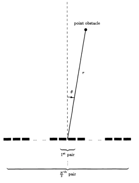
In this investigation, it is assumed that the point target and all the transducers lie in the same plane as illustrated in Figure 2 for N =4transducers. Uniformly spaced sensors in this array are modeled as identical Polaroid sensors pointing in the same direction. Both of these assumptions can be relaxed without significant change in the following development.

Suppose there is a point target located at (x, j)andthat the i'th transducer transmits a pulse whose mathe-matical model will be provided in the next section. The rectangular coordinates of the i'th and j'th transducers, where i, j =1,...,

N,

are (x ,0)and (x, ,0)respectively as shown in Figure 2 for N =4. Improved distance-of-flight (DOF) estimation is performed by matched filtering'0 in place of thresholding.' The DOF measured at transducer i is f, and the corresponding DOF at j is f3. These DOF's at the two transducers define a circle and an ellipse whose point of intersection with a positive y coordinate corresponds to the target location. With the DOF measurement at the transmitter, the target can lie anywhere on the circle defined by

(x—x,)2+y2=f,

(1)

Similarly, for the receiver, the point-target can correspond to any point on the ellipse described by

—

2/

2

—1 2

f2 _{[f — (r,—z,)} —

If

the above equations are solved for target coordinates x and y:

=

_{2fj(fj±fi)+xi+xj}

₍₃₎

2

=

₍₄₎

One of the two roots x1,2 is chosen as x such that f, —_(x—

x2)2 is positive. Using x and y, the target polar coordinates can be found as

r =

#'x2y2

9

=

sin

()

₍₅₎

3 ESTIMATING THE POINT-TARGET LOCATION

3.1 Description of the two methods

Using the given array configuration, information from the sensors can be fused in a number of ways. Earlier,

finding the optimal receiver separation at a given range for plane-corner differentiation and choosing the pair that best approximates this separation in a linear array of N transducers has been investigated.2 With the same configuration, fusing information pairwise from all pairs of receivers symmetric around the center of the array has been considered and the 'optimal' weighting factors for the estimates from these pairs has been found.2 This method improved the accuracy of the estimates approximately by 10% although the processing time was increased threefold for N = 6. This method will be referred as the sub-array method since it does not make use of all the received signals available in the system.

In the array configuration assumed here, every transducer takes turn in transmitting, and after each traris— mission, received waveforms are recorded at every transducer. Hence, after a full cycle of transmission, there are N2 received waveforms. This allows the extension of the sub-array method to a more complete one in which every available echo is used. In total, there are N(N —1) such pairs from which both 8 and r estimates can be obtained as explained in the previous section. This method will be referred as the pairwise esiimaie (PE) method. Although this extension makes more complete use of the acquired data in localizing the point target, a single, robust location estimate needs to be extracted from the data. From the geometry of Figure 2, r and 0 estimates are obtained (given by Equation 5) at each receiver when one of the N transducers is used as a transmitter. One way of combining these N(N —1) estimates is to first calculate their expected values and standard deviations. Those estimates that are not within two standard deviations are excluded and the mean is recalculated, providing a more robust estimate (the PE). An improved estimate could be obtained by a weighted combination of the pairwise estimates where the weights change depending on the separation between the transmitter and receiver as well as range and azimuth.

In a second approach, all received waveforms are considered at the same time and the best r and 9 which provide the most probable fit (the MLE) to the acquired data are chosen as the final estimate. This procedure requires the use of nonlinear iterative optimization techniques. Since the cost function used in this optimization procedure is observed to have multiple local minima, the choice of the starting point is important in reaching the optimal values. One good choice is the minimum of the cost function on a coarse mesh centered around the PE result. The minimum so obtained is used as an initial estimate to find an approximation to the MLE of rand9 by minimizing the cost function described below. In this work, MATLAB constraint optimization routine is used which employs second order derivative information to find the minimum of the cost function.

Let us assume the following additive noise signal-observation model for our system:

r(tk,z)

=

_s,(tk,Z)

₊

_{nlj(tk) (6)}

for i, j

=

1, ...,

N

and k = 1, ..., M.Here, r2(tk) is the received waveform at time sample tkatthe j'th transducer

when the i'th transducer is activated. The vector z is the location parameter vector of the point-target given by

(7)

s (2k,r, 0)is modeled as follows:

r, 8) =

A(x1,r, 8) A(x,, r, 8) G(x,r, 8) G(x,, r, 8)M[tk — t(r,8)— t3(r, 8)] cos{2irf0{ik —t(r, 8)—_{t3(r, 8)])(8)}

where

A(z,r,0) =

1 (9)

2ir[r2 cos2 9 + (r sin 0 —_x2)2]3

2J ka

(rsin9—a,) 1 G(x,r,9)

=

ka (10) Jcos2 8+(rsin8—x1)2 M[t]

= exp (-)

rect

(L!)

(11) SPIEVol. 2561 / 535

i(r, 9) =

%/r2cos2 0 +(r sin 9 —

x)2

(12)

wherek =_2!:, the speed of sound in air, and f, =50kHz is the resonant frequency of the Polaroid transducer

which has aperture radius a =2_{cm. Here, A(x ,r,}9) is the free-space attenuation factor of pressure amplitude,

G(x,

r,0) is the gain pattern of the transducer, and M[t] is the envelope of the waveform modeled as a gated Gaussian. The duration of the pulse is approximately 85 ,us, corresponding to five periods of the sinusoid. Time-controlled gain amplifiers are commonly employed to compensate for the spreading loss due to diffraction and attenuation in air,11 so that the reflection amplitude can be considered to be independent of range.

Note that the received waveform has nonlinear dependence on range and azimuth. It is desirable to have unbiased r and 0 estimates based on the acquired array data. In this type of nonlinear estimation problems, it is difficult to find an exact expression for the variance of the estimate. In the following section, the performance of any nonlinear unbiased estimator will be characterized by deriving a lower bound for its variance.

3.2 Derivation of the Cramér-Rao lower bound

Cramér-Rao Lower Bound (CRLB) defines a lower bound on the variance of any unbiased estimator.3 To find the CRLB in this particular case, an independent identically distributed Gaussian noise model is assumed with the following conditional probability density function:

NNM

2

TT iT r-r 1 [r(ik) —

PrIz('Iz) =

;L[1;L[1 M

exp—

_q2

(13)

The MLE estimate given above chooses that value of z which maximizes the conditional probability. By taking the natural logarithm of both sides, a simpler expression to be maximized is obtained:

lnprlz(rlz) =

{ln

— [r12(ik)—8s2(ik,Z)]2

}

(14) From above, the final form of the cost function to be minimized for the MLE is

{r(i)

—sIj(tk,z)}2

(15)

i,j,k

Due to the nonlinearity of the expression in z, an exact expression for the MLE is difficult to find. The MLE procedure used in this paper iteratively minimizes the cost function. Also, from this expression the CRLB can be derived by computing the following partial derivatives of Equation 14

Olnpriz(rlz) —— ç—[r1(tk) —sj(tk,z)}Osjj(tk,z) o.2

Oz

ô2 _{— c;—'} {r1(ik) —

_sj

_{(tk, z)J 02sz3 (ik, z)}

+

—-- c ôs2j (ik,z) Os,, ₁₆ — OZnOZm —

.2

OZnOZm q2 Ld OZrn

where the righthandside for n, m = 1,2 defines the entries of J, the Fisher Information Matrix.3 Then the

expected value of J is:

E{J} =H ₍₁₇₎ where 1 _{Osjj(tk,z) OsI,(tk,z)}

Hn,m =—

( ) _o.2

n,m=

t9zm 1 2 ₍₁₈₎ z,j ,k 536ISPIE Vol. 2561

&t1(r,O) — 8r t1(r, 0) — 80

j

1

Then, the CRLB becomes

E{(—z)2}

_H'(n,n)

(19)

Here, is any unbiased estimate of the parameter vector elements r and 9. In evaluating Equation 18, the first term in Equation 16 drops out and the second term remains.

To find the expressions in Equation 16, partial derivatives of the amplitude and gain terms are evaluated and simplified to:

8A(x, ,r,0)

_{_}

r

— x sin9

8r _{2/ir[r2 cos2 0 + (rsin0 —}

8A(v,r,0)

₌

_ xrcos0

80 _{2i./ir[r2 cos2 0 + (rsin0 — s)2]3}

8G(s,r,8) ka [o(kisin0') — J2(kasin0') _{2J1(kasino')l} sinG _{(rsin0 — s)(r — s sinG) 1}

8r I ka sin0' _{(ka sin 01)2} J _{cos2 0 + (r sin 0 — s)2 [r2}cos2 0 + (r sin 0 — x)2]3/2

8G(s,r,0) _{k [Jo(ka si.nO')}—J2(ka sin0') 2J1(ka sin0')l

r

cos 0 (r sinG — s1)(rx cos 8)

00 a kasin8' _{(kasin0)2j /r2cos28+(rsin8_s)2 + Er2cos2O+(rsinOx)2]3/2]}

_______ 2(r— x sin 6)

cJr2 2srsin6+s

_______ —2srcos6 (20)

csrsin0+s

I rsin0—s

where 6 =

ka

,/;:

9 (rsin6 —

In the next section, performances of both of the PE and MLE for point-target localization will be investigated and compared to the CRLB over some synthetic test cases.

4 RESULTS AND DISCUSSION

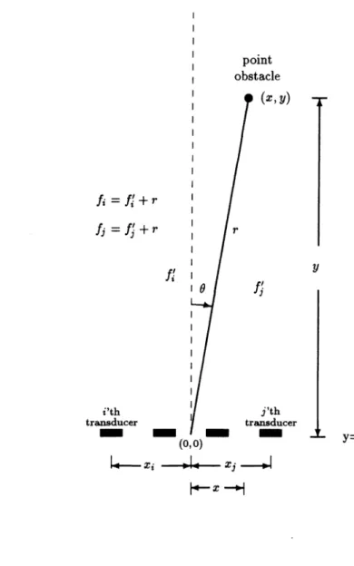
The results presented in this section are obtained from a simulation study for an array of N =4transducers of Polaroid sensors with resonant frequency f, = 50 kHz and separation 6 cm. The minimum allowed separation is 4 cm corresponding to placing the transducers of diameter 4 cm side by side. Based on the results of our earlier experiments,2 the chosen separation provides good target resolution up to ranges of 2 m. For simplification purposes, the reception pattern of the transducer is computed at the resonant frequency, neglecting the effect of the narrow bandwidth around fe,. In this case, the beam pattern of the transducer is modeled as a first-order Bessel function of the first kind as illustrated in Figure 3.

Figure 4 displays received waveforms at each transducer when the leftmost one transmits. The point target is located at a range of r = 1 m and an azimuth of 0 40• Thestandard deviation of the artificially-added Gaussian noise is chosen to be 5% of the maximum signal amplitude at a range of 1 m, hence a signal-to-noise ratio (SNR) of approximately 26 dB corresponding to (r, 0) =_(im,0°). Figure 5 shows the corresponding waveforms when the range is changed to 4 m with the same azimuth. Although both figures have the same amount of noise, Figure 5 looks more noisy since the relative amplitude of the waveforms received at r =4 m to noise is 16 times less than that at r =1 m due to free-space attenuation modeled in Equation 9.

In this simulation study, statistical performances of the two methods (PE and MLE) are compared with each other as well as with the CRLB derived previously. Each of the N(N —_{1) pairs provides a single range}

and azimuth estimate. The mean values and standard deviations of these estimates are computed based on ten different realizations for a given range and azimuth. Figure 6, shows the standard error of the range and azimuth estimates that are obtained from PE and MLE when the azimuth is kept constant at 9 =_O, and the range r is changed between 1—4 m with 25 cm increments. The standard error is found by summing the squares of standard deviation and the bias of the estimate and then taking the square root. Both of these approaches indicate similar trends. The standard deviation of MLE in r is slightly more than that of PE. The slight increase in the standard deviations as r increases is due to the decrease in the SNR because of the free-space attenuation factor. For comparison purposes, the ClUB for unbiased estimators has also been included in each figure. It is not possible to make a comparison to the CRLB for biased estimators since an analytic expression for the bias is not available. The estimation bias partially derives from that one already present in the raw DOF measurements since these measurements are obtained by thresholding.1 Although these standard deviations have an increasing trend as a function of r, even at r =4 m, their values are of the order of 1 cm in r and approximately 0.1° in 0. These values are acceptable in practice.

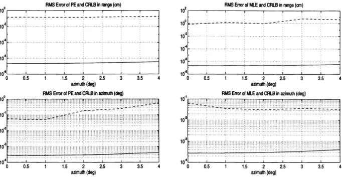
The results obtained when r is kept constant at 2 m and 9 is varied between 0 —4°with increments of 1° is illustrated in Figure 7. All of the above observations apply to these two cases as well. In this case, the increasing trend with 9 is due to the reduced transducer gain as a function of increasing O.

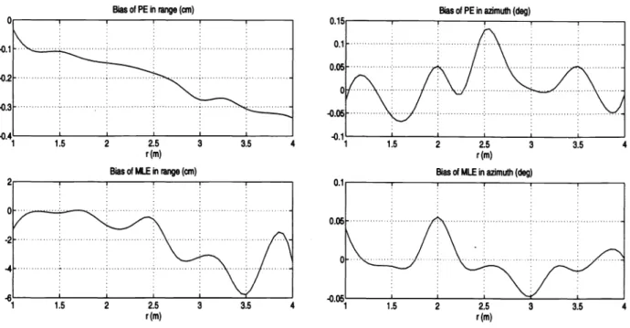
Biases of these estimates have also been investigated based on the same set of simulations. The results are shown in Figures 8 and 9. In the first figure, biases of PE and MLE as function of r have been displayed when C is kept constant at O . Fora better display, the data points have been fitted with a spline. The bias in estimating range as a function of r in both cases is acceptable, at worst 5.9 mm. Corresponding biases in the azimuth estimates are also within the acceptable range of for PE and for MLE. In the second figure, biases as functions of C are investigated at a constant range of r =2m. Again, the available data has been interpolated by a spline fit. All of these biases are also within acceptable levels.

Based on this simulation study, it has been observed that although in estimating range, both PE and MLE perform comparably, MLE is superior in estimating the azimuth of the point target.

5 CONCLUSION

Two different methods of combining information from a linear array of N acoustic transducers for estimating the position of a point target have been described and simulated. The methods are characterized by small biases, and standard errors larger than the CRLB by an order of 2—4. Although the PE and MLE methods provide similar range estimation accuracy, MLE outperforms the PE in estimating azimuth. This study is useful for characterizing the point-target response of acoustic sensors and forms a basis to find their response to rough surfaces which can be modeled as a random collection of point targets.

6 ACKNOWLEDGEMENTS

This work was supported by TUBITAK EEEAG-92 project.

— — —

.

1st pair

Nth

T pair

point obstacle

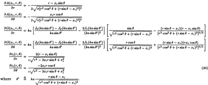
Figure 1: A linear transducer of N transducers for obstacle localization.

SPIE Vol. 2561 / 539

0

r

point obstacle (x,y) i'th j'th transducer transducer

—

— — —

(0,0) I4—Xj 1d11 ci J$ 10

f=f+r

Ii =f+r

r

y ci J2

L y=O

Figure 2: A linear array of N =4transducers for obstacle localization.

Beam Pattern

theta (deg)

Figure3: Transducer beam pattern at the resonant frequency f0 =50kHz.

Amplitude

57 5.75 5.8 5.85 5.9 5.95 6 6.C

time(s) x 1O

Figure 4: Received waveforms at each transducer when r=1 m.

Amplitude

mAfrAM/mwv

0.0232 0.0232 0.0233 0.0233 0.0234 0.0234 0.0235

time(s)

Figure 5: Received waveforms at each transducer when r=4m.

Figure 6: RMS errors of PE and MLE in range and azimuth as a function of rindashed line when 0 =0°. CRLB

in solid line.

1 1.5 2 2.5 3

azimuth(deg)

RMSError of PE andCALB1n azimuth (deg)

1 1.5 2 2.5 anmuth (deg)

Figure 7: RMS errors of PE and MLE in range and azimuth as a function of 0indashed line when r= 2 m. CRLB in solid line.

542/ SPIE Vol. 2561

RMS Errorof PE andCRIBin range (cm)

100

102

jo.4 106

RMS Error ofMLEand CRIB inrange (cm)

,.-.-10•1 10. 10. 10 1 1.5 2 2.5 3 3.5 r(m)

RMS Errorof PE and CRLBin azimuth(deg) .!!!I 1 1.5 4 102 100 102 101 1 1.5 2 2.5 3 3.5 r(m) 0 SffOrofMLEW1dCRLBinlIThith(deg) 10 10_i .::'::: ::::._.• ::.::...::.:.:....::...:

225335_4

_r(m) 2 2.5 r(m) 3 3.5

RMS Errorof PE and CRIB in range (cm)

100 I I I I

102

101

.8

RMS Error of MLE and CRIB in range (cm)

102 100 102 iü• 0.5 3.5 100 101 io.2 101o 0.5 1 I I I I I 0.5 1 1.5 2 2.5 3 3.5 azimuth (deg)

RMS Errorof MIE and CRIB in azimuth (deg)

101 I I I I I 102 .:: 10.:: . .: :::::::..::: : : .I::..:.::..::::.:..::...::....:.::::::.:. ::.• 1 I I I I I I I 4 0 3 3.5 0.5 1 1.5 2 azimuth (deg) 2.5 3 3.5 4

Bias of PE in azimuth (deg) o.1c I I

Figure 8: Biases of PE and MLE in range and azimuth as a function of rwhen0 =00.

Bias of PE in range (cm)

4N\N,

-0.13

0.5 1 1.5 2 2:5 3 3.5 4

azimuth (deg) Bias of MLEinrange (cm)

0 0.5 1 1.5 2 2.5 3 3.5 4

azimuth (deg)

Bias of PE in azimuth (deg)

0

05 115 2

25 1

azimuth (deg) Bias ofMLEin azimuth (deg)

"0

0.5 1 1.5 2 2.5 3 3.5 4

azimuth (deg)

Figure 9: Biases of PE and MLE in range and azimuth as a function of 0 when r= 2m.

SPIEVo!. 2561 /543

Bias of PE in range (cm)

14

1.5 2

r(m)

2.5 3 3.5 Bias of MLE in range (cm)

1.5 2 2.5

r(m)

3 3.5

Bias of MLE in azimuth (deg)

r(m)

I 1 I I I I I

7 REFERENCES

[1] B. Barshan. A Sonar-Based Mobile Robot for Bai-Like Prej Capture. PhD thesis, Yale University, New Haven, CT, December 1991. University of Michigan Microfilms, order number 9224325.

[2] B. Barshan and R. Kuc. Differentiating sonar reflections from corners and planes by employing an intelligent

sensor. IEEE Transactions on Paflern Analjsis and Machine Intelligence, 12(6):560—569, June 1990. [3] H. L. Van Trees. Detection, Esiimaiion, and Modulaiion Theory, Part I. John Wiley & Sons, New York,

1968.

{4] H. Peremans, K. Audenaert and J .M.Van Campenhout. A high-resolution sensor based on tn-aural

per-ception. IEEE Transactions on Roboiics and Aniomaiion, 9(1):36—48, February 1993.

[5] J. J. Leonard and H. F. Durrant-Whyte. Mobile robot localization by tracking geometric beacons. IEEE Transactions on Robotics and Automation, 7(3):376—382, 1991.

[6] J. Zemanek. Beam behaviour within the nearfield of a vibrating piston. The Journal of the Acoustical Society of America, 49(1 (Part 2)):181—191, January 1971.

[7] K. Sasaki and M. Takano. Classification of object's surface by acoustic transfer function. In Proceedings IEEE/RSJ International Conference on Intelligent Robots and Systems, pages 821—828, Raleigh, NC, July

7—10, 1992.

[8] M. L. Hong and L. Kleeman. Analysis of ultrasonic differentiation of three-dimensional corners, edges and planes. In Proceedings IEEE International Conference on Robotics and Automation, pages 580—584, Nice,

France, May 12—14, 1992.

[9] 0. Bozma and R. Kuc. Characterizing pulses reflected from rough surfaces using ultrasound. Journal of the Acoustical Society of America, 89(6):2519—2531, June 1991.

[10] P. M. Woodward. Probability and Information Theory with Applications to Radar. Pergamon Press, Oxford,

1964.

[11] Polaroid Corporation. Ultrasonic components group. 119 Windsor St., Cambridge, MA 02139, 1990.