A comparison of two methods for fusing information from a linear array of sonar sensors for obstacle localization

(1)

A Comparison of two Methods for Fusing Information from a

Linear Array of Sonar Sensors for Obstacle Localization

*

Orhan Arikan and Billur Barshan

Department

of

Electrical Engineering

Bilkent University

Bilkent,

06533

Ankara, Turkey

_;

point

,

obstacle

Abstract

The performance of a commonly employed linear array

of sonar sensors is assessed f o r point-obstacle localiza- tion intended f o r robotics applications. T w o different methods of combining time-of-flight information from the sensors are described to estimate the range and az-

imu-th of the obstacle: pairwise estimate method and the maximum likelihood estimator. The variances of

the methods are compared

t o

the Cram&-Rao Lower Bound, and their biases are investigated. Simulation studies indicate that in estimating range, both methods perform comparably; in estimating azimuth, maximum likelihood estimate is superior

at

a cost o f extra com- putation. The results are useful for target localization in mobile robotics.

1 Introduction

In this paper, the performance of a commonly employed linear array of sonar sensors is assessed for point-target localization. Characterizing point-target response of a sensor has been important not only for its application to point targets but also to assess its performance on extended targets which can be modeled using different approaches [l, 2 , 31. If the approach is one of hypothesis testing or one of parametrizing the extended target, then sensor performance may not be easily related to its point-target response. On the other hand, for extended targets of unknown shape with possible roughness

[4],

or for small spherical targets, point target analysis can be extremely useful. Aside from modelling extended targets, the point target analysis can be easily extended to spherical targets of finite radius which may be of interest in robotics applications. In this study, only point targets are considered. By implementing a multi-transducer system that exploits the differences in the signal travel times and combining information from the array elements, the location of a point target can be accurately esti- mated in two dimensions.

In the next section, the transducer model and the linear array configuration are described. In Sec- tion 3 , two different approaches for point target localization are described and the CramCr Rao Lower Bound

(CRLB)

is derived. The performances of the

*This work was supported by TUBITAK EEEAG-92 project.

I

Y

1

y=o

Figure 1: A linear array of N = 4 transducers for localization.

two methods are discussed in terms of bias and variance, and their variances are compared t o the CRLB

in Section 4. In the concluding section, the usefulness of the methods is assessed for point-target localization.

2 The Sensor Model and the Array

A single acoustic transducer can be employed both as a transmitter and receiver. After the transmitted pulse encounters an object, an echo is detected by the

same transducer acting as a receiver. In this study, the excitation is chosen to be a gated Gaussian-modulated sinusoid. Localization of a point target is performed in the far-zone of the transducer where the propagating pulse is considered t o be a series of plane waves.

In this investigation, it is assumed that the point target and all the transducers lie in the same plane as illustrated in Figure 1 for N

=

4 transducers. Uni- formly spaced sensors in this array are modeled as

(2)

identical Polaroid sensors pointing in the same direc- tion. Both of these assumptions can be relaxed with- out significant change in the following development.

Suppose there is a point obstacle located at ( x , y) and that the i’th transducer transmits a pulse whose mathematical model will be provided in the next section. The rectangular coordinates of the i’th and j ’ t h transducers, where

i,

j =

1,

...,

N ,

are

(xi,

0) and ( x j , O ) respectively as shown in Figure

1

for

N

=

4.

The distance-of-flight (DOF) measured a t transducer

i

is fi, and the corresponding DOF at j is fj. These DOF’s at the two transducers define a circle and an ellipse whose point of intersection with a positive y co- ordinate corresponds to the obstacle location, Solving for the intersection point:

One of the two roots x1,2 is chosen as x such that

f;”

-

(x

- xi)2 is positive. Using x and y, the polar coordinates of the target can be found as

r =

Jm

(3

0 = sin-’ (3)

3 Estimation

of

Point-Target Position

3.1 Description

of the two Methods

Using the given array configuration, information from the sensors can be combined in a number of ways. In earlier work, finding the optimal receiver separation at a given range for plane-corner differentiation was considered and the pair that best approximates this separation in a linear array of N transducers was chosen [5]. With the same configuration, fusing information pairwise from all pairs of receivers symmetric around the center of the array have been investigated and the ‘optimal’ weighting factors for the estimates from these pairs were found [5]. This method im- proved the accuracy of the estimates approximately by 10% although the processing time was increased threefold for N = 6. This method will be referred as the s u b - a r r a y method since it does not make use of all the received signals available in the system.

In the array configuration assumed here, every transducer takes turn in transmitting, and after each transmission, received waveforms are recorded a t every transducer. Hence, after a full cycle of transmission, there are N 2 received waveforms. This allows us to extend the sub-array method to a more complete one in which every available echo is used. In total, there are N ( N - 1) such pairs from which b o t h

6’ and T estimates can be obtained [5]. This method will be referred as the p a i r w i s e e s t i m a t e

(PE)

method. Although this extension makes more complete use of the acquired d a t a in localizing the point obstacle, a

single, robust location estimate needs t o be extracted

from the data. From the geometry of Figure 1, T and 6‘ estimates (given by Equation 3) are obtained at each receiver when one of the N transducers is used as a

transmitter. These N ( N - 1) estimates are combined

by calculating their mean and excluding any estimate not within two standard deviations of the mean while doing so.

In a second approach, all received waveforms are considered at the same time and the best r and 0

which provide the most probable

fit

(the MLE) to the acquired data are chosen as the final estimate. This procedure requires the use of nonlinear iterative optimization techniques. Since the cost function used in this optimization procedure is observed to have mul- tiple local minima, the choice of the starting point is important in reaching the optimal values. One good choice is the minimum of the cost function on a coarse mesh centered around the PE result. The minimum

so obtained is used as an initial estimate to find an approximation to the

MLE

of r and

0

by minimizing the cost function described below.

The following additive noise signal-observation model is assumed:

r i j ( t k , z ) = S i j ( t k , z )

+

n i j ( t k ) (4)

for i , j = 1, ..., N and k = 1,

...,

M . Here, r i , ( t k ) is

the received waveform at time sample t k at t i e j ’ t h

transducer when the i’th transducer is activated. The vector z is the location parameter vector of the point- target given by

(11)

~2 cos2 6’

+

( T sin 6’ - x i ) z t i ( T ’ 8 ) = J

C

where IC =

y ,

c is the speed of sound in air, and fo = 50 kHz is the resonant frequency of the Polaroid transducer with aperture radius a = 2 cm. Here, A(xi,r,B) is the free-space attenuation factor of the pressure amplitude,

G

xi! T , 0) is the gain pattern of the transducer, and M

i

t ]

is the envelope of the waveform modeled as a gated Gaussian.

(3)

Note that the received waveform has nonlinear de- pendence on range and azimuth. I t is desirable to have unbiased r and 6' estimates based on the acquired array data. In this type of nonlinear estimation prob- lems, it is difficult t o find an exact expression for the variance of the estimate. In the following section, the performance of any nonlinear unbiased estimator will be characterized by deriving a lower bound on its variance.

3.2 Derivation

of

t h e

Cram&-Rao

Cram&-Rao Lower Bound (CRLB) defines a lower bound on the variance of any unbiased estimator [6]. To find the CRLB in this particular case, an inde- pendent identically distributed Gaussian noise model is assumed with the following conditional probability density function:

Lower Bounds

!la) The MLE estimate given above chooses that value of z which maximizes the conditional probability. By taking the natural logarithm of both sides, we obtain

a simpler expression to be maximized:

From above, the final form of the cost function t o b;? minimized for the MLE is

Due t o the nonlinearity of the expression in z , an ex- act expression for the MLE is difficult to find, and an

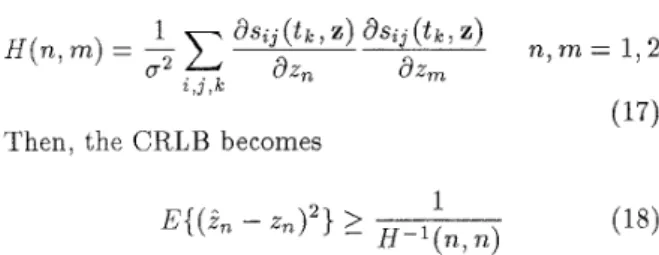
iterative numeric method is used. From the above expression the CRLB can be derived by computing the following partial derivatives of Equation 13

- d21npriz(rlz) =

-E

[ T t J ( t k ) - S 2 3 ( t k ) Z ) ] a 2 s t j ( t k , z ) az,az, U2 az,az, r , 3 , k ( 1 5 ) 1 a s L j ( t k , Z ) a S , J ( t k , Z )

+,.E

32, az77l C , J , 1 :

where the righthandside for n , m = 1 , 2 defines the entries of J , the Fisher Information Matrix [6]. Then the expected value of J is:

E{J} = H (16)

where

Here, Z is any unbiased estimate of the parameter vector elements r and 6'.

To find the expressions in Equation

15,

partial derivatives of the amplitude and gain terms in Equa- tion 8 were evaluated.

Beam Pattern

3

Figure 2: Transducer beam pattern at the resonant frequency fo =

50

kHz. 0.1 Amplitude I 32 0.0232 0.0233 0.0233 0.0234 0.0234 0.0235 time(s) Figure 3:

when r=4 m. Received waveforms a t each transducer In the next section, performances of both of the

PE and MLE for point-obstacle localization will be investigated and compared t o the CRLB over some synthetic test cases.

(4)

4 Results and Discussion

The results presented in this section are obtained from a simulation study for an array of

N

= 4 transducers of Polaroid sensors with resonant frequency

fo = 50 kHz and separation 6 cm. Neglecting the

narrow bandwidth around f o , the beam pattern of the

transducer is a first-order Bessel function of the first kind as illustrated in Figure 2.

Figure 3 displays received waveforms at each transducer when the leftmost one transmits. The point obstacle is located at a range of r = 4m and an azimuth of 0 = 4”. The standard deviation of the added Gaussian noise is chosen to be 5% of the maximum signal amplitude at a range of 1 m .

In this simulation study, statistical performances of the two methods ( P E and MLE) are compared with each other as well as with the CRLB derived previ- ously. Each of the N ( N -

1)

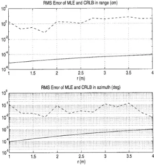
pairs provides a single range and azimuth estimate. The mean values and standard deviations of these estimates are computed based on ten different realizations for a given range and azimuth. Figure 4, shows the standard error of the range and azimuth estimates that are obtained from P E when the azimuth is kept constant at B = 0”,

and the range r is changed between 1-4 m with 25 cm increments. The standard error is found by summing the squares of standard deviation and the bias of the estimate and then taking the square root. The corresponding results for the MLE are given in Figure 5. Both of these approaches indicate similar trends. The standard deviation of MLE in

r

is slightly more than that of P E . The slight increase in the standard deviations as T increases is due to the decrease in the signal-to-noise ratio because of the free-space attenuation factor. For comparison purposes, the CRLB for unbzased estimators has also been included in each figure. It is not possible to make a comparison t o the CRLB for bzased estimators since an analytic expression for the bias is not available. The estimation bias partially derives from that one already present in the raw DOF measurements since these measurements are obtained by thresholding [7]. Although these standard deviations have an increasing trend as a function of r , even at

r

=4 m , their values are of the order of

1

cm in T and approximately 0.1” in 8. These values are acceptable in practice.

The results obtained when T is kept constant a t 2 m and B is varied between 0 - 4” with increments of

1” is illustrated in Figures 8 and 9. All of the above observations apply to these two cases as well. In this case, the increasing trend with B is due to the reduced transducer gain as a function of increasing

/el.

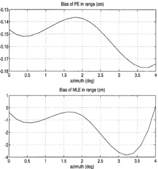
Biases of these estimates have als0 been investigated based on the same set of simulations. The results are shown in Figures 6, 7, 10 and 11. In the first two figures, biases of

PE

and MLE as function of r have been displayed when B is kept constant at

0”. For a better display, the d a t a points have been fitted with a spline. The bias in estimating range as a function of r in both cases is acceptable, at worst 5.9

mm. Corresponding biases in the azimuth estimates are also within the acceptable range of f 0 . 1 4 ” for PE and f 0 . 0 5 5 ” for MLE. In the last two figures, biases

as functions of 6’ are investigated at a constant range of T = 2 m . Again, the available d a t a has been in- terpolated by a spline

fit.

All of these biases are also within acceptable levels.

Based on this simulation study, it has been observed that although in estimating range, both

PE

and MLE perform comparably, MLE is superior in estimating the azimuth of the point target.

5 Conclusion

Two different methods of fusing inforrnation from a linear array of N acoustic transducers for estimating the position of a point target have been described. The methods are characterized by small biases, and standard errors larger than the CRLB by an order of 2-4. Although the P E and MLE methods provide similar range estimation accuracy, MLE outperforms the P E in estimating azimuth.

This study is useful for characterizing the point- target response of acoustic sensors and forms a basis to find their response to rough surfaces which can be modeled as a random collection of point targets. The system is being implemented in hardware and the obtained experimental results will be compared with the analytical and simulation results. The results are useful for target localization in mobile robotics.

References

[1] H. Peremans, E(. Audenaert and J. M. Van Camp- enhout

“A

high-resolution sensor based on tri- aural perception,” IEEE Transactions on Robotics and Automation, vol. 9, pp. 36-48, February 1993. [2] J . J . Leonard and H. F. Durrant-Whyte “Mobile robot localization by tracking geometric beacons,” IEEE Transactions on Robotics and Automation, [3] M. L. Hong and L. Kleeman “Analysis of ultra- sonic differentiation of three-dimensional corners, edges and planes,” in Proceedings IEEE Inter- national Conference on Robotics and Automation, pp. 580-584, Nice, France, May 12-14, 1992. vol. 7, pp. 376-382, 1991.

[4]

0.

Bozma and

R.

Kuc “Characterizing pulses reflected from rough surfaces using ultrasound,” Journal of the Acoustical Society of America, vol. 89, pp. 2519-2531, June 1991.

[SI B. Barshan and

R.

Kuc “Differentiating sonar re- flections from corners and planes by employing an intelligent sensor,” IEEE Transactions on Pat- tern Analysis and Machine Intelligence, vol. 1 2 , pp. 560-569, June 1990.

[6] H. L. Van Trees. Detection, Estimation, and Mod- ulation Theory, Part

I.

John Wiley

&

Sons, New York, 1968.

[7] B. Barshan.

A

Sonar-Based Mobile Robot for Bat- Like Prey Capture. PhD thesis, Yale University,

Ncw Haven, CT, December 1991. University of

(5)

RMS Error of PE and CRLB in range (an) Bias of PE in range (cm)

I I I I I

1.5 2 2.5 3 3.5 4

r (m)

RMS Error of PE and CRLB in azimuth (deg)

- i

. , , , , . . . . . . .

I I I I I I

1 1.5 2 2.5 3 3.5 4

r (m)

Figure

4:

RMS error of PE in range and azimuth as a function of range when B = 0" in dashed line. CRLB

in solid line.

RMS Error of MLE and CRLB in range (an)

102, I I

,

I

, - _ _ _ _ - - - _ _ - / - -

- -

- - < ' IO0

.;

' . I , _ - - . . I 1 o-2

I

' " 1 1.5 2 2.5 3 3.5 4 r (m)

RMS Error of MLE and CRLB in azimuth (deg)

__---

i

-

:&---

I

i

I

,

I I I 1 1.5 2 2.5 3 3.5 4 rim) 10-"1

Figure

5:

RMS error of MLE in range and azimuth as a function of range when 0 = 0" in dashed line. CRLB in solid line.

"I

I I

,

I I

1 5 2 2.5 3 3 5 4

r (m) Bias of MLE in range (cm)

-i I

-2 -

-4-

-"l 1.5 2 2.5 3 3.5 4

r (m)

Figure 6: Bias of P E and MLE in range as a function of range when B = 0".

Bias of PE in azimuth (deg)

,

I I I I I

4 41'

1 1 5 2 2 5 3 3.5

r (m) Bias of MLE in azimuth (deg)

OO;i.L---JL

0

4

1 1 5 2 2 5 3 3.5 4

-0.05

r (m)

Figure 7: Bias of PE and MLE in azimuth as a function of range when B = 0".

(6)

lo-*

'" 0 0.5 1 1.5 2 2.5 3 3.5 4

azimuth (deg)

RMS Error of PE and CRLB in azimuth [deal

- . ". r--- _,

_ _ - - -

_ _ _ _ _ _ _ . .. . - - - - lod- Bias of PE in range (cm) -0.131 I I

1

I I I I I

,

1 azimuth (deg) Bias of MLE in range (cm)

I " 0 0.5 1 1.5 2 2.5 3 3.5 4

azimuth (deg)

Figure 8: RMS error of P E in range and azimuth as a function of azimuth when r = 2 m in dashed line. CRLB in solid line.

RMS Error of MLE and CRLB in range (cm)

_ - - - - _ _ _ - _

IO'/

i

0 0.5 1 1.5 2 2.5 3 3.5 4

azimuth (deg)

Figure 9: RMS error of MLE in range and azimuth as a function of azimuth when r = 2 m in dashed line.

CRLB in solid line.

Figure 10: Bias of P E and MLE in range as a function

of azimuth when r = 2 m .

Bias of PE in azimuth (deg)

-0 41

\

-0.6 I I I I I I I

0 0 5 1 1 5 2 2 5 3 3 5

azimuth (deg) Bias of MLE in azimuth (deg)

O O 2 I

-0.021 I I I

,

I

,

I I

0 0.5 1 1.5 2 2.5 3 3.5 4

azimuth (deg)

Figure 11: Bias of PE and MLE in azimuth as a func- tion of azimuth when r = 2 m.