Gaussian mixture models design and applications

Μ Ο Β Έ ί Λ

;J*· ;; '•ί·.'^»..·' ,.>1·.·^; _{V i ÎÂ'ı^. ■}-Tb·; *· _{i %}5*·.·ϊ!

_{Т Н і}

2 7 ^ , 4

’J S 4 ^ z o c o

GAUSSIAN MIXTURE MODELS DESIGN AND

APPLIGATIONS

A THESIS

SUBMITTED TO THE DEPARTMENT OF ELECTRICAL AND ELECTRONICS ENGINEERING

AND THE INSTITUTE OF ENGINEERING AND SCIENCES OF BILKENT UNIVERSITY

IN PARTIAL FULFILLMENT OF THE REQUIREMENTS FOR THE DEGREE OF

MASTER OF SCIENCE

By

Khaled Ben Fatma

I certify that I have read this thesis and that in rny opinion it is fully adequate, in scope and in quality, as a thesis for the degree of Master of Science.

“

h i ·

A. Ellis Çetin, Ph. D.(Supervisor)

I certify that I have read this thesis and that in my opinion it is fully adequate, in scope and in quality, as a thesis for the degree of Master of Science.

Billur^Barshan, Ph.

I certify that I have read this thesis and that in my opinion it is fully adequate, in scope and in quality, as a thesis for the degree of Master of Science.

/ I / / r\ -/./

Yasemin "^rdimci, Ph. D._{f ,·'} vy

Approved for the Institute of Engineering and Sciences: Prof. Dr. Mehrnet B ^ ^ '

Director of Institute of Engineering and Sciences

WA -2 M -4

~В4б Л о а о

ABSTRACT

GAUSSIAN MIXTURE MODELS DESIGN AND

APPLICATIONS

Khaled Ben Fatma

M.S. in Electrical and Electronics Engineering

Supervisor: A. Enis Çetin, Ph. D.

January 2000

Two new design algorithms for estimating the parameters of Gaussian Mix­ ture Models (GMh-l) are developed. These algorithms are based on fitting a GMM on the histogram of the data. The first method uses Least Squares Error (LSE) estimation with Gaus,s-Newton optimization technique to provide more accurate GMM parameter estimates than the commonl}' used Expectation- Maximization (EM) algorithm based estimates. The second method employs the matching pursuit algorithm which is based on finding the Gaussian func­ tions that best match the individual components of a GMM from an over- complete set. This algorithm provides a fast method for obtaining GMM pa­ rameter estimates.

The proposed methods can be used to model the distribution of a large set of arbitrary random variables. Application of GMMs in human skin color density modeling and speaker recognition is considered. For speaker recognition, a new set of speech fiiature jmrameters is developed. The suggested set is more

appropriate for speaker recognition applications than the widely used Mel-scale based one.

Kexjxoords'. Gaussian Mixture Models, Parameter Estimation, Expectation-

Maximization Algorithm, Gauss-Newton Algorithm, h/Iatching Pursuit Algo­ rithm, Least Sciuares Error, Speaker Recognition.

ÖZET

GAUSS KARIŞIM MODELLERİNİN TASARIMI VE

UYGULAMALAR

Khaled Ben Fatma

Elektrik ve Elektronik Mühendisliği Bölümü Yüksek Lisans

Tez Yöneticisi: Prof. Dr. A. Enis Çetin

Ocak 2000

Gauss Karışım Modellerini (GMM) parametrelerinin kestirimi amacıyla iki yeni tasarım algoritması geliştirilmiştir. Bu algoritmalar veri histogramı uy­ durma yoluna dayanmaktadır. Birinci yöntem, GMM parametre k(!stiriminde alışılagelmiş Ixiklenti en büyükleme (EM) algoritması tabanlı kestirimlerden daha doğru sonuçlar sağlamak için Gauss-Newton eniyilerrıe tekniğiyle en küçük kareler hata k(!stirimini (LSE) kullanmaktadır, ikinci yöntem, sözlük olarak ad­ landırılan, aşırı tamamlanmış Gauss modelleri kümesinden bir GMM’in her bir bileşenini en iyi eşleyim Gauss işlerlerini bulmak için kullanılan uyum izleme algoritmasına dayanmaktadır. Bu algoritma GMM parametre kestirimi için hızlı bir yöntem sunmaktadır.

Önerilen yöntem geniş bir rasgele değişken kümesini modellemekte kul­ lanılabilir. GMM’lerin kullanım alanı olarak insan deri renk yoğunluğu mod- ellemesi v(î konuşmacı tanıma problemleri seçilmiştir. Konuşmacı tanıma için yeni bir konuşma öznitelik parametre kümesi geliştirilmiştir. Ongörühm

bu yeni küıiK!, yaygın olarak kullanılan Mel-skala tabanlı küni(;ye kıyasla konuşmacı tanımaya daha uygundur.

Anahtar Kelinuder: Gauss Karışım Modelleri, Parametre Kestirimi, Bcîkhmti

En Büyükleme Algoritması, Gauss-Newton Algoritması, Uyum İzleme Algorit­ ması, En Küçük Kareler Hatası, Konuşmacı Tanıma.

ACKNOWLEDGMENTS

I would like to express my deep gratitude to my supervisor Prof. Dr. A. Enis Çetin for his supervision, guidance, suggestions and patience throughout the devel­ opment of this thesis.

I am grateful to Dr. Yasemin Yardımcı for her valuable suggestions and help which contributed a lot to the progress of this thesis. Special thanks to Dr. Billur Barshan for reading and commenting on the thesis.

I thank all of my friends for their sincere friendship throughout all these .years. It is a pleasure to express my special thanks to my father, mother, and sisters for their love, support, and encouragement.

C on ten ts

1 Introduction 1

2 Gaussian Mixture Models (GMM) 5

2.1 Description 5

2.2 Applications of G M M ... 6 2.3 GMM Parameter E stim ation... 7 2.4 Expectation Maximization (EM) Algorithm 8

3 Least Squares Error (LSE) Estimation 10

3.1 Least Squares Data Modeling 11 3.2 GMM Parameter E stim ation... 13 3.2.1 Gaus.s-Newton Algorithm... 15 3.2.2 Algorithmic Issues 17

3.2.3 Simulatioi) Studies 19

3.3 An Application 20

3.4 Conclusions 22

4 Matching Pursuit Based GMM Estimation 25

4.1 Matching Pursuit A lgorithm ... 26

4.2 Matching Pursuit Based E stim ation... 27

4.3 Fast C alcu latio n s... 30

4.4 Experimental Results and D iscussion... 31

5 Speaker Recognition Using GMM and a Nonlinear Frequency Scale 33 5.1 Mel-Frequencj^ Cepstral Coefficients... 34

5.2 New Nonlinear Frequencj' S c a le ... 36

5.3 Subband Decomposition (Wavelet) Based Computation of Fea­ tures ... 39

5.4 Experimental Study and C onclusions... 41

5.4.1 Database D escription... 41

5.4.2 Experimental R.(;!sults... 41

6 Conclusion ₄₃

APPENDICES ₄₆

A RGB to CIELUV Color Space Conversion ₄₆

A.l CIELUV Color S p a c e ... 46 A.2 RGB to XYZ Conversion... 47 A.3 XYZ to CIELUV Conversion... 47

List o f Figures

3.1 Two typical realization of the parabolic fit of the error function with the corresponding minimum value... 19 3.2 Mean square error obtained for GMM estimation using

GN(straight line) and EM (dashed line) algorithms, (a) 1-D GMM, M =4, (b) 1-D GMM, M=12, (c) 2-D GMM, M=A, (d)

2-D GMM, M=12. 20

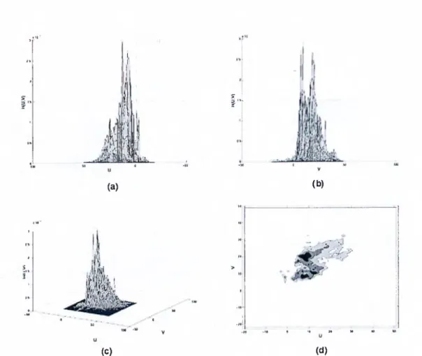
3.3 Human skin color pdf estimation, (a) original image, (b) skin pixels extracted for GMM training. 22 3.4 2-D human skin color histogram in the UV space seen from

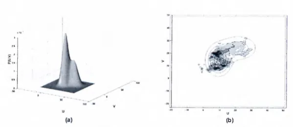
different angles...,... 23 3.5 Estimated human skin color density function using EM algo­

rithm, (a) 3-D view of the estimated histogram, (b) Top view of estimated histogram compared to the histogram shown in Figure

3.4d. 23

3.6 Estimated human skin color density function using Gauss- Newton algorithm, (a) 3-D view of the estimated histogram, (b) Top view of estimated histogram compared to the histogram

shown in Figure 3.4d... 24

3.7 Skin color estimation squared error obtained at each iteration using EM algorithm, Gauss-Newton algorithm with normal per­ turbation step size and Gauss-Newton algorithm with estimated optimum perturbation step size... 24

5.1 Triangular bins arranged on a Mel-scale for MFCG features ex­ traction... 35

5.2 A sampling scheme for filter banks which is more sensitive to a.ccent characteristics... 37

5.3 Speaker identification performance based on the energy in dif­ ferent frequency bands... 37

5.4 A new frequency axis division suitable for speaker recognition applications... 38

5.5 Pre-emphasis applied to speech frames... 39

5.6 Basic block of a subband decomposition... 39

5.7 Subband decomposition approximation to Mel-scale... 40 5.8 Frequency scale for speaker recognition using subband decom­

position. 40

List o f Tables

4.1 Speaker identification rate using EM algorithm and the match­ ing pursuit algorithm. The model training time corresponds to a set of 30 speakers and 40 sec speech signals per speaker. 32 5.1 Center frequencies (Hz) of triangular windows shown in Figure

5.4... 38 5.2 Speaker identification performance for different frequency do­

main scales using MFCC and SUBCEP features... 42

C hapter 1

In trod u ction

In nature, observed phenomena tend to have a wide variety of non-uniform dis­ tributions that often are very hard to estimate or model. In signal processing, modeling the distribution of an arbitrary phenomenon is a primordial step in understanding and analyzing the behavior of that phenomenon.

Gaussian Mixture Models (GMM) have been recently used in many appli­ cations as an efficient method for modeling arbitrary densities [1]. A Gaussian mixture density is defined as a weighted sum of different Gaussian component densities. GMMs were shown to provide a smooth approximation to the under­ lying long-term sample distribution of observations obtained from experimental measurements [1]. This is mainly due to the fact that a linear combination of Gaussian basis is capable of representing a large class of sample distributions, in addition to the observation that most natural phenomena tend to ha.ve a Gaussian distribution.

There are several techniques available for estimating the parameters of a GMM [2], [3], [4]. By far the most popular and well-established method is maximum likelihood (ML) estimation. The aim of ML estimation is to find the model parameters that maximize the likelihood of the GMM, given the training data. This usually leads to a nonlinear global optimization problem. ML parameter estimates can be obtained in an iterative manner using a special case of the Expectation-Maximization (EM) algorithm [5]. The EM algorithm is an iterative algorithm, which starts with an arbitrary model and tries to obtain a better model at each iteration until convergence in some sense is reached. The EM algorithm usually leads to good estimates of the GMM parameters. However, it does not always provide accurate estimates of the GMM parameters. Moreover, its computational complexity makes it unsuitable for applications where speed is important such as real time and adaptation applications.

New methods for estimating the parameters of a GMM by curve fitting to the histogram of the observation data are introduced. Two methods are described; one is based on least squares error estimation using Gau.ss-Newton algorithm and the other is based on the matching pursuit algorithm.

The least squares error method tries to obtain the best parameters by mini­ mizing an error function over the unknown parameters. A parameter separation technique is used to simplify the optimization procedure [12]. The resulting er­ ror function is a highly nonlinear function of the parameters, the Gauss-Newton algorithm is used to obtain an iterative estimate to the problem. This method provides more accurate estimates resulting in a better model. Moreov(>r, it needs a v('iy few number of iterations to converge.

The second method is based on the matching pursuit algorithm. Pursuit algorithms are generally used to decompose arbitrary signals [15]. Decompo­ sition vectors are chosen depending upon the signal properties. Vectors are selected'one by one from a dictionary, while optimizing the signal approxima­ tion at each step. In this thesis, a modified version of the matching pursuit is used as an alternative method for estimating the parameters of a GMM. This method has a lower accuracy than the EM based method, but its low com­ putational complexity makes much faster and more suitable for applications where speed is crucial such as adaptation algorithms [27], [28], and real time applications.

Speaker recognition is an important application where the use of GMMs has proven to be very efficient [1], [10]. Speaker recognition can be divided into two sub-fields: Speaker Identification which tries to identify the person speaking an utterance from a known set of speakers, and Speaker Verification which tries to check wh(!ther a speaker is that who he claims to be or is an impostor. For both of these tasks, many models like Hidden Markov models (HMMs), Midtiple Binary Glassiher Model (MBCM), Neural Networks, etc.. [10], ai(i proposcxl. GMM is recognized as one of the most accurate models for Automatic Spcuiker Recognition (ASR), using telephone speech [1]. The speech spectrum basoid parameters are very effective for speaker modeling. The most widely used speech feature parameter set is based on the Mel-scale cepstrurn. Tin; Mel-scale based features produce excellent results for speech recognition, as the Mel-scale division of the spectrum is compatible with the human auditory system. This spectrum division may not be the best possible division for speaker recognition applications. In this thesis, we propose a new set of features that is more appropriate to speaker recognition applications.

This thesis is organized as follows. In Chapter 2, we describe briefly the general form of a GMM and the EM algorithm used for estimating its param­ eters. In Chapter 3, we develop the idea of using least squares data modeling implemented Iry the Gauss-Newton algorithm to derive more accurate GMM parameter estimates. An application of this idea is also described. Chapter 4 presents a fast GMM parameter estimation method based on a modified ver­ sion of the matching pursuit algorithm. Speaker recognition is considered in Chapter 5, where a new set of speech feature parameters is proposed. Finally, conclusions are given in Chapter 6.

C hapter 2

G aussian M ixtu re M odels

(G M M )

2.1

D escription

Given an arbitrary Z)-dimensional random vector f , a Gaussian mixture density of M components is defined as a weighted sum of individual D-variate Gaussian densities i = 1, as follows

M

p(f|A) = Y ^ P i k (f) _(2.1) z=l

where p,:, i -- are the weights of the individual components and are constrained by

M

E ” · = 1 (2.2) z=l

The D-vai'iat(' Gaussian function h i { x ) is given by

hr{x) = - exp <: - ^ (f - 1 fii)' T.· ' (f - /1,;) (2.3) 5

where /i^ is tlui mean vector and E,; is the covariance matrix. Therefore a GMM can be rei)resented by the collection of its parameters A as

A = = (2.4)

The GMM can have different forms depending on the choice of the co- variance matrices. The covariance matrices can be full or diagonal. Because the component Gaussians are acting together to model the overall probability density function, full covariance matrices are not necessary even if the observa­ tions are statistically dependent. The linear combination of diagonal covariance Gaussians is capable of modeling the correlations between the observation vec­ tor elements. The use of full covariance matrices can significantly complicate the GMM estimation procedure, while the effect of using M full covariance Gaussians can be approximated by using a larger set of diagonal covariance Gaussians.

2.2

A pplications of GM M

Gaussian mixture models have been used in many applications as an efficient method for modeling arlntrary densities. Since a GMM is capable of modeling a broad range of pi obability densities, it has found use in a very large area, of applications. In [7] for example, the probability density function of human skin color was estimated using a GMM. The estimated probability density function has many applications in image and video databases. These applications range from hand tracking to human face detection. Similarly in [8], an object tracking algorithm is developed using GMMs. Gaussian mixture models were used to estimate the ])robability densities of objects foreground and scene background

colors. Tracking was perfonned by fitting dynamic bounding boxes to image re­ gions of maximum probabilities. GMMs have been also used very effectively in speaker recognition for modeling speaker identity [1], [10]. Short-term speaker- dependent feature vectors are obtained from the speech signal, then Gatissian mixture modeling is used to estimate the density of these vectors. The use of Gaussian mixture models for modeling speaker identity is motivated by the interpretation that the Gaussian components represent some general speaker- dependent spectral shapes and the capability of Gaussian mixtures to model arbitrary densities.

2.3

GM M Param eter E stim ation

Given an observation sequence X - f>^C)m a random vector x, the goal is to estimate the parameters of the GMM A, which in some sense best matches the distribution of the observation data. This GMM can then be considered as a valid estimate to the distribution of the random vector x.

There are several techniques available for estimating the parameters of a GMM [2], [3], [4]. By far, the most common and popular method is maximum likelihood (ML) estimation [5]. This method tries to find the model parameters that maximize the GMM likelihood

T

p ( . i |A ) = n p ( a |A ) (2.5) i=l

given the training vectors X . This leads to a nonlinear function of the param­ eters A and direct minimization is not possible. However, ML estimates ca,n

be obtained in an iterative manner using the Expectation-Maximization (EiM) algorithm [5]. The EM algorithm is described in the next subsection.

Another possilrle method for the estimation of the GMM parameters A, is to trj' to make a smooth fit to the histogram of the observation sequence A'” using a linear coml)ination of Gaussian functions. This idea will be further investigated in later chapters. Two new methods using this idea will be presented along with some possible applications.

Usually there are two important factors in training of a GMM: model or­ der selection and parameter initialization for iterative methods. We will not address these problems in this thesis.

2.4

E xpectation M axim ization (EM ) A lgo­

rithm

The EM algorithm tries to find the estimates of the ML parameters iteratively. It begins with an initial model A, and tries to estimate a better model until some convergence is reached. In each EM iteration, first a posteriori probability is estimated as

= (2.G)

L·k=ı Pkh [xt)

Based on this jn-obability, mixture weights, means and variances are estimated using the following re-estimation formulas, which guarantee a monotonie in­ crease in the model’s likelihood value:

Mixt/are weights:

Pi = i = l , . . . , M (2.7)

i=l.

where p, is the new e.stimate of the ?;th mixture weight and it is obtained by a.veraging all a posteriori probability estimates.

Means:

7^ _ 'YJt=\P{AiL·t■,

p. =

E f = iP ( 'la .^ )

(2.8)

where /7 is the new estimated mean vector of the ¿th mixture. Variances;

^2 ^ _ .2

>.9) where a'f refers to new estimates of arbitrary entries on the diagonal of the covariance matrix and :ct, pi refer to the corresponding elements of the vectors Xf and ~p.

In many applications, the EM algorithm has shown satisfying results . How­ ever, it does not always provide accurate estimates and it may converge to bad local maxima. Better estimates can usually be obtained for the same model under consideration. Moreover, the computational complexity of the EM algo­ rithm is relatively high especially when the training set is large [6].

C hapt er 3

Least Squares Error (LSE)

E stim ation

In the previous chapter, we described how ML estimation can be used to obtain estimates to the parameters of a GMM through the EM algorithm. In this chapter, we discuss the estimation of the parameters of a GMM Iry trying a least squares fit to the histogram of the observation data. Given an olrservation sequence X — , ■■■■■Lt·, }> obtain the normalized histogram H[x).

We want to use H (x) to obtain a Gaussian mixture estimate to the unknown distribution of X of the form

M

= J 2 pA {x) (3.1)

i=l

where A represents the model parameters and the weights Pi are constraiiKid by E f : , w = i·

We start by ex])ressing the histogram as

M

H(x) = + 10(f) (3-2)

i=\

where w{x) is the error l)etween the histogram and the Gaussian mixture den­ sity to be estimated. In other words, we express the histogram of the observa­ tion data as a linear combination of Gaussian functions bi{x).

We use the least squares data modeling to estimate the parameters of the GMM. This is done by minimizing a given function of the estimation error

’w{x). We use the Least Squares Error (LSE) criterion. The Gauss-Newton

algorithm is later used to obtain estimates to the unknown parameters in an iterative manner.

We first present a brief review of the basic concepts of least squares data modeling, then we proceed to its application in GMM parameter estimation.

3.1

Least Squares D ata M odeling

In many applications, the observed signal or sequence is often assumed to be composed of a linear combination of “basis functions” which are characterized by a set of ])arameters, and additive noise [11]. The observation vector of length N is given by

M

h^Y^Pibi{9i)

where p, is the coefficient of ith basis vector bj{0j), which depends on the parameter vector while w is the additive error sequence. This expressio))

can also Ixi written in the compact form

h = B{6)p + w

where B{0) is a N x M Irasis matrix given by

(3.4)

(3.5)

p is the vector containing the M coefficients and 6 is the composite parameter

vector

« = [ € « r . i t ] ' (3.6)

The objective is to select the unknown parameter vectors 9 and the amplitude set p so that the linear combination of the basis functions best fits h. Using the LSE criterion we have to minimize the functional

e(^,p) = \ \ h - B { 9 ) ^ \ (3.7) This is a highly nonlinear optimization problem with no closed from solution, therefore nonlinear programming techniques are necessary to achieve the opti­ mization.

To make the optimization problem in (3.7) simpler, we note that the func­ tion to be minimized has two important properties:

• The unknown parameters 9 and p are separable.

• The least squares error criterion e{9,p) is a quadratic function of the amplitudes

p-For problems with these properties, Gloub and Pereyra [12], proposed a parameter se])aration technique to ease the complexity of the problem. The

idea is to fiml tlui optimum amplitude vector in terms of the unknown paramete.rs 9. Then the set of unknowns reduces to the vector 9. Once these are found, the o])tirnum amplitude vector j f can then be obtained directl}^ This parameter separation tcichnique simplifies the computations and significantly improves the speed of convergence.

To obtain an expression of the optimum amplitude vector in term of the unknown parameters 9, we first use the QR decomposition to write basis matrix

B{9) in the form

B(9) = Q{9)R{9) (3.8)

where Q{9) is a N x M orthonorrnal matrix and R{9) is a M x M nonsingular upper triangular matrix. The expression for the optimum amplitude vector is formulated in [11] and given by

/ = R{0 )-^Q{ 0fh . (3.9) The corresponding least squares error criterion’s value for this optimum choice is given by

е Ц У ) = ! f h - h^Q[0)Q{9fh. (3.10) By minimizing criterion (3.10), we obtain the vector of the unknown parameters

Once this vector has been found, it is substituted into expression (3.9) to obtain the corresponding amplitude vector j f .

3.2

GM M Param eter E stim ation

In our ai)])lica,tion, we want to estimate a density function that fits the distri­ bution oi' a s(4|uenc:e of observed data, as a mixture of Gaussian functions. To

use least s(}uares data modeling, we have to put expression (3.2) in the form of expression (3.4). For 1-D case, this is straightforward:

M h = '^PгbiX0i) + w (3.11) 1=1 B {0)p + w where: (3.12)

P = b i P2 ■·· PmY is the mixture weights vector.

6j — [p,i is the parameter vector of the zth Gaussian component and

B(0)

-

bi {^Xi, )

bl{X2,0M)

blixN,ii) bi{xM,02) · · · bi{xN,0n^)

In our model, we use diagonal covariance matrices. Expression (3.9) gives us the optimum weights vector as

/ = R{0)-^Q{0fh.

where Q{0) and R{ff) are obtained from QR decomposition oi B{&).

(3.1.3)

This approach can be extended to higher dimensions in a similar manner. The observation vector h can be obtained by putting the columns of H{x) into one vector seijuentially, R(^) can be then obtained accordingly.

The minimization piol:>lem (3.10) is highl}^ nonlinear in the unknown vector therefore nonlinear programming techniques must be used to achieve the opti­ mization. For this task, we use the Gauss-Nev'ton algorithm developed in [11], which is a descent method that has proven to be very effective in solving highly nonlinear programming problems. In typical iterative optimization techniques, the parameter vector is incrementally perturbed so th at the cost criterion takes lower values at each iteration. In other words, the current parameter vector в/. is perturbed to obtain

(ЗЛ4) where S,. is the perturbation vector which is chosen in such a wa.y that a decrease in the cost criterion results.

In Gaus.s-Newton algorithm, the optimum perturbation vector 61, which results in the highest decrease in the cost criterion, is estimated at each iter­ ation. This procedure ensures that quadratic or superlinear convergence rates are attained in a neighborhood of a relative minimum.

For the nonlinear optimization problem given in (3.4), the Gauss-Newton perturbation vector at the kth iteration is given by

3 .2 .1 G a u s s - N e w to n A lg o r ith m

=

--1

(.3.15) where J {(h.) is the Jacobian matrix and the residual vector e(p",^/J is given by

= (3.10)

■J il) =

The Jacobian matrix, J { ( f ) lias the form

de. (3.17)

The partial derivative terms are approximated as

A

- _ A ;

where is a projection matrix defined as Pq_ = Q{e)Q{9)^.

(3.18) (3.19)

The algorithm starts with an initial estimate 0_o of the unknown parameters. At each iteration of the Gauss-Newton algorithm, the optimal perturbation vector is used to update the parameters vector e_o so that an improvement in the criterion (3.10) is obtained

h+ \ - + “ fcii/c· (3.20)

The step size a.k is selected large at earl}'^ iterations and reduced at later stages of the optimization procedure. Usually, a*, is chosen from the sequence

= 1 i i i

‘ ’ 2 ’ 4 ’ 8 ’ ·" (3.21) until the first value of a.k which reduces the cost criterion is found. Once the parameter vector 9 is found, it is inserted in expression (3.13) and the amplitude set p" is obtained.

Initialization

One critical i'actor in GMM parameter estimation is the initialization of the model parameters. The initialization procedure is verj^ important for the per­ formance of the Gauss-NeAvton algorithm. It was checked experimentall}· that a bad initialization can result in high estimation error and a poor model. One efficient initia.liza.tion method consists of randomly choosing vectors from the training data as mean vectors followed by /f-means clustering to initialize means, variances and mixture weights.

Optimum Step Size

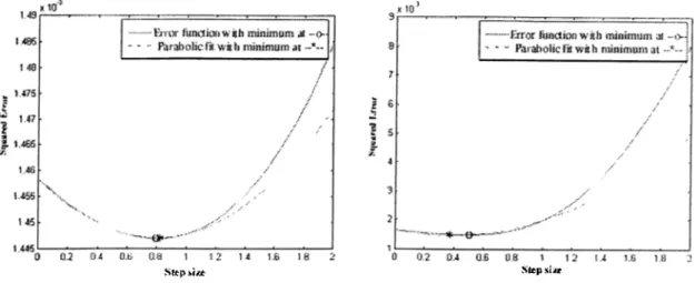
In subsection 3.2.1, we discussed how the step size used in expression (3.20) can be chosen from the sequence in Equation (3.2 1). This procedure can be effective in finding an appropriate step size that results in a decrease in the error criterion for a. given perturbation vector. However, it does not find the best possible step size that results in the highest decrease in the cost criterion. Since the calculation of a perturbation vector 6^ is relatively costly in computation power, we wa,nt to get the most out of this perturbation vector once it is calculated by estimating the corresponding step size that results in the highest decrease in the error criterion. Here, we introduce a procedure! lor estimating the optimum step size al for a given perturbation vector. We start by considering the error function to be minimized given in Equation (3.7), which is the sciuared error between the normalized histogram and tlu' estimated distribution. Once a. new ])erturbation vector is calculated the new A-alue of this

3 .2 .2 A lg o r ith m ic Issu e s

error funelioii depends on the stejr size a.k , denoted by e(a'fc). We want to find the value ofo!^ for which c(o;^) < e(o;^.), for all 0 < < 1. For these values of Qifc, it was found oixperimentally that the error function can be approximated by a paralrola as

= «-«fc + FttA- + C 5 0, G IR. For this ])arabola the minimum value is given for

h < = - 2a

(3.22)

(3.23) To fit a parabola to e{a.k) we need its value at three different point of between 0 and 1. We use the region 0 < Q!^: < 1, because we do not want to get too far from our current operating point (a* = 0), since far from this point the error function is unpredictable and our approximation becomes invalid. We already know c(0) which is the error value at the previous iteration so need two more points. We use e ( l /2) and e(l), this is enough to find the parameters a, and c of the parabola. We equate the values of e{ak) and e(ak) at a*; = 0,1 /2,1. Then the three following equations gives us the solution:

(3.24) e(0) = c a 2 - 4 2 ■ e(0) ■

e{^) = ^<’· + + c h - 3 4 - 1

e(l) = a + b c c 1 0 0

We plug the values of a and b into Equation (3.13) to obtain

b 3e(0) - 4 e (l/2 )+ e(l)

at = (3.25)

2o. 4[e(0) - 2e ( l /2) + e(l)]·

This gives us an estimate for the best step value a;°.. Some typical experimental realization of this method are shown in Figure 3.1. The results in Fignix' 3.1 show that our approximation is valid around the region 0 < a;*; < 1. The estimated optimum stej) size is very close to the correct one.

vStfcf» sii«· Step siiw

Figure 3.1: Two typical realization of the parabolic fit of the error function with the eorr(ispoii(ling minimum value.

3.2.3

Sim ulation S tu d ies

In this subsection, simulation studies are carried out to compare the perfor­ mance of the suggested method with the EM algorithm. For this purpose, data from Gaussian mixture densities are generated at random. Simulations were carried out for both 1-D and 2-D GMMs. For each Gaussian mixture, 2000

observations are gxmerated and used to obtain an estimate to the parameters of the original distribution. The estimation error criterion is defined as

2

=

T

4-cornponent and 12-component mixtures are used. For each experiment, 100

runs were made and the mean square error of the 100 runs is computed. The 100 runs are also divided into 10 groups of 10 runs such that in each group of 10 runs the GMM parameters are kept constant but 10 different sets of observations are generated, from which the histogram is computed. Figure 3.2 shows the

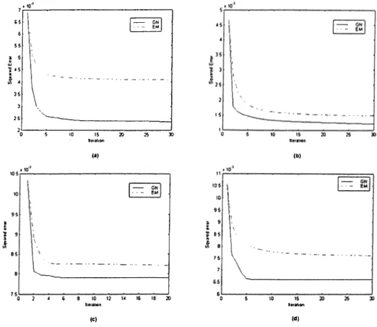
results for the 1-D and 2-D cases corresponding to 4 and 12 component GMMs. 7 6 55 2 5 lU ■₂S *5 4 35 3 25 2 15 20 Nmlioo (·) (b) lltrAliOti <C) h*rMl»n (d)

Figure 3.2; Mean square error obtained for GMM estimation using GN(straight line) and EM (dashed line) algorithms, (a) 1-D GMM, M =4, (b) 1-D GMM, M =12, (c) 2-D GMM, M =4, (d) 2-D GMM, M =12.

3.3

A n A pplication

Probabilit}' density modeling using GMMs have been used in a wide range of applications ranging from speech and image processing to biology. In this

section, we consider some simple recent applications of GMMs to test the per­ formance of the proposed Gauss-Newton based parameter estimation method compared to the EM-based one.

In [7], a probability density function of human skin color was estimated using a Gaussian mixture model whose parameters were estimated through the EM algorithm. The estimated density function has many applications in image and video databases. These applications range from human face detection to hand tracking.

A set of experiments similar to those described in [7] were carried out to estimate a probability density function of human skin color, but in our case the estimation of the GMM parameters was done using both the EM algorit.hm and the Gauss-Newton based method and the results are compared.

Typical human skin pictures were collected and human skin regions were extracted manuallj'. A sample is shown in Figure 3.3. Each sample (skin color pixel) consists of three values (R,G,B). To reduce the dependence on the light­ ing condition, each sample is transformed from RGB to CIELUV color space and then the brightness component is discarded. The color space transfor­ mation from RGB to GIELUV in given in Appendix A. Figure 3.4 shows the resulting 2-D histogram of skin color (histogram of x = {u,v)‘^ ).

As in [7], two Gaussian components were used to estimate the probability density function corresponding to the histogram shown in Figure 3.4. Figure 3.5 and Figure 3.6 show the estimated densitj^ function for EM and Gauss- Newton methods respectivel}^ The corresponding estimation squared error is shown in Figure 3.7.

(a) (b)

Figure 3.3: Human skin color pdf estimation, (a) original image, (b) skin pixels extracted for GMM training.

From Figure 3.5 and 3.6, we can see that the Gauss-Newton method results in a better model then the EM algorithm. This is confirmed by Figure 3.7 since the estimation squared error is smaller in the case of the Gauss-Newton estimation. Figure 3.7 also shows the improvements in performance obtained when using the optimum step size described in 3.2.2.

3.4

C onclusions

In this chapter, we described Gauss-Newton optimization technique based ap­ proach to obtain the parameters of a Gaussian Mixture Model. We experimen­ tally demonstrated that this method provides a more accurate representation of the data compared to the widely used EM algorithm. Furthermore, this method often converges in less number of iterations.

'I· ■ft I'tt'i .y*,

11

(a)

I w

(b)

Figure 3.4: 2-D human skin color histogram in the UV space seen from different angles. 1 * 1 , i 1 / 1 ■ ^ ) j : , , 1 I fT'lki I i * * ' ' . . . . - ' " ' i 1 « ’ ' ■ ·· - , - ■ · ' ■ ' - i t - _{. . . . . : . . . .} . 1 0 4 » to M « t * u (a) U (b)

Figure 3.5: Estimated human skin color density function using EM algorithm, (a) 3-D view of the estimated histogram, (b) Top view of estimated histogram compared to the histogram shown in Figure 3.4d.

M ^ ·

-10 0 ;o

1/

(b)

Figure 3.6: Estimated human skin color density function using Gauss-Newton algorithm, (a) 3-D view of the estimated histogram, (b) Top view of estimated histogram compared to the histogram shown in Figure 3.4d.

xIO 4.1 4 -3.9 -\ !3.83.7 3 .6 3 .5 -3.4 L

1 :

GN with optimum step size GN with normal step size

4 5

iteration

10

Figure 3.7: Skin color estimation squared error obtained at each iteration using EM algorithm, Gauss-Newton algorithm with normal perturbation step size and Gauss-Newton algorithm with estimated optimum perturbation step size.

C hapter 4

M atch in g P u rsu it B ased G M M

E stim a tio n

In this chapter, we develop a fast method for obtaining GMM parameter esti­ mates for arbitrar}^ probability densities. This method is based on the matching pursuit algorithm. As in Chapter 3, we use the histogram of the observation data for deriving our model. The matching pursuit algorithm is used to de­ compose the histogram into different Gaussian functions. This decomposition results in a Gaussian mixture density that can be used as an estimate to the probability density of the random vector under consideration. In section 4.1, we start by giving a brief description of the matching pursuit algorithm. The suggested method is presented in section 4.2.

Matching pursuit is a recently proposed algorithm for deriving signal-adaptive decompositions in terms of expansion functions chosen from an over-complete set called a dictionary -over-complete in the sense that the dictionary elements, also called atoms, exhibit a wide range of behaviors [13]. Roughly speaking, the matching imrsuit algorithm is a greedy iterative algorithm which tries to determine an expansion for an arbitrary signal a:[n] given a dictionary of atoms,

g-y[n], as follows

K

x[n] = ^a . k g ^ \ n ] (4.1)

k=\

where the dictionary is a family of vectors (atoms) g^ included in a Hilbert space H with a unit norm ||^.y|| = 1 and 7 is the set of parameters characterizing g^.

4.1

M atching P ursuit A lgorithm

Matching pursuit algorithms are largely applied using dictionaries of Ga.- bor atoms [14]. Gabor atoms are appropriate expansion functions for time- frequency signal decomposition, which are a scaled, modulated, and translated version of a single unit-norm window function, g{.), which has the following form in continuous-time domain

(4.2) where 7 is the collection of parameters 7 = (s,iJ.,e) € F = R"''x R^. Note that

g^, is centered in a neighborhood of /i whose size is proportional to s and its

Fourier transform is centered at u = s. This parametric model provides mod­ ification cai)abilities for time and frequency localization properties of signals.

4.2

M atching P ursuit B ased E stim ation

We want to use the matching pursuit algorithm with Gabor atoms to find a suitable decomposition to the speech features histogram. In our application, the modulation factor e'~'' in expression (4.2) is not necessary since the fre­ quency localization has no meaning in this case, and thus it is dropped and we use

(4.3) Furthermore, if we choose g{t) as a Gaussian function of zero mean and unit variance then we obtain ' 23^'’ , = \/s.Ai{n, s^) (4.4) (4.5) (4.6) which is a Gaussian function with mean /r and variance scaled by a factor

^/s. The discrete form of (4.5), is

(/yM = 1 exp - -/ in N — ¡xY' (4.7) where and N is the sampling period. The resulting g^[n] is a suitable decom­ position function for our application.

In the following, we introduce a fast method for estimating the param­ eters of a GMM using the matching pursuit algorithm with decomposition functions derived in (4.7). Given an arbitrary D-dimensional random vcic-tor X .Tj X'> ■ · · xdvr\ , wei want to obtain a Gaussian mixture chmsitv

which api)roximat,es the distribution of .f, using a set of observation vectors A' = •••>^7··, }■ Let us first write A as

A = X l •i^'2.1 ■ ■ '^2,2 ^2.T = X2 ■ C £),l ^D,T . . (4.8)

where Xi , i = I, ...,D are the sequences of training data corresponding to each of the D components of x. For each A',;, we calculate the corresponding 1-D normalized histogram Hi{x). If we can decompose Hi{x) into a finite weighted sum of Ganssian components, we obtain a valid estimate to the distribution of ,Xi, the 'ith component of x. The decomposition is done as follows. We first define our dictionary D as a family of vectors g^. The form of is given in (4.7). Each decomposition vector g^ depends on the parameter 7 = (p-, *)· The range of // can be obtained from the range of Hi{x), while the range of

s should be chosen experimentallJ^ The dictionary should be large enough to

cover a wide range of vectors. The algorithm starts by finding g^^ 0 ^ ^ best matches Hi{x) in the sense that the inner product q)|, which is a

measure of similarity between Hi{x) and gry^ ,^, is maximized, i.e.,

\ { H i , g j i , o ) \ > sup |(i7i,5^)|. (4.9)

Then, we can write

Hj i?7i,0 T RHi (4.10) where RHi is the residual vector. The iteration then proceeds on RHi as the initial vector. Supjoose that R^'Hi denotes the r¿th residual of Hi , at the ?7,th iteration we get

R"H, = (4.11)

If we cany the iteration to order M, we obtain 77. = 0 M-l — ^ ‘^Í,n!J'n,n + Hi (4.12) (4.13) n=0

where and 7,;„, = (/¿¿,71,6',:,„,)· This gives us a decompo.sition of Hi{x) as a weighted sum of Gaussian components. Let’s examine the first term of the RHS of Equation (4.12). From Equation (4.5) we obtain

M-l M-l

7?. = 0 7?,=0

If we further define the weight pi^n

Piji —E M - lJvl -

n =

(4.14)

(4.15)

0 Y

•^2,n'-*'2,77-SO that ~ r tlien we obtain a valid Gaussian mixture model for .x·,;

M - l

p{^i\K) = '^Pi,nh,n{^i) (4.16)

7г=0

where hi^n{x) is a Gaussian with mean g.i^n and variance both obtained from the decomposition of Hi{x).

If we carry out this procedure for all the individual components of x, then we obtain D separate 1-dimensional models corresponding to the D components of .x: Xi , i = For 1-dimensional signal, this procedure results in one GMM that can be used as a model for the distribution of that signal. However, in higher dimensional cases the resulting 1-D models cannot be used to obtain the overall distribution directly, unless the individual components of the random vector are uncorrelated. For this case, the overall Z)-dimensionaJ GMM can be obtained by multiplying the individual 1-D GMMs

D

p(,f|A) = flp (ii|A ,;). (4.17)

¿-1

For random variables with correlated components, this is not valid. One possible solution is to applj' a. transformation that decorrelates or at least iTiinimizes the correlation between the individual components of x. In speech processing for example, a Discrete Cosine Transform (DCT) is used to decor­ relate the speech feature obtained from a speech signal. A DCT or a similar transform can be used to decorrelate (or at least minimize) the correlation be­ tween the individual components of the random vector. In this case, expression (4.17) can be used to obtain a good estimate to the overall distribution of the random vector.

In the next section, a fast calculation method is proposed to increase the algorithm’s speed.

4.3

Fast Calculations

The matching pursuit can be implemented using a fast algorithm described in [23], that computes from {R^Hi,gy) with a simple updating-formula. Consider Equation (4.11), which we can write as

Take the inner ]noduct with g~,. on each side, we obtain

(4.18)

{rr*'H„a„) = {R'‘H.,g,) -

(o is)

which is a simple updating formula for Hi, gy). If we can calculate the

inner product of all the atoms in the dictionary, {ga,(j0), ^i^nd store it in a lookup table, then we can use this update formula to calculate {RJ'^^Hi,gy) a.t each iteration. The final algorithm is summarized below:

For eac.li //,; , i —

1. Set 77, = 0 and compute

2. Find r;^,„ G V such that; (/^.„)| > sup \{H,,g^)\ for all 7 G F 3. Update for all g^^ ,^,^ G V:

4. If n < M — 1 increment n and go to 2.

4.4 E xperim ental R esults and D iscussion

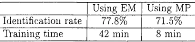
Even though the proposed method provides a less accurate model then the EM algorithm for random variables with correlated entries, its low computational complexity makes desirable. This method is especially useful for applications where speed is important. We have tried the matching pursuit based method in the application of speaker identification and the rates of recognition were compared to those obtained using the EM algorithm. Table 4.1 summarizes the results for a 30-speaker set with a training sequence of 40 sec for each speaker. The simulations were carried out on an Intel-Pentium based PC using MATLAB. The rates of identification in the matching pursuit case are h;ss than those for the EM algorithm. However the model training time for the 30-speaker set is extremely lower than that required by the EM algorithm.

Using EM Using MP Identification rate 77.8% 71.5% Training time 42 min 8 min

Table 4.1: Speaker identification rate using EM algorithm and the matching pursuit algorithm. The model training time corresponds to a set of 30 speakers and 40 sec speech signals per speaker.

C h ap ter 5

Speaker R ecogn ition U sin g

G M M and a N on lin ear

F requency Scale

In general, the field of speaker recognition can be classified into two sub-areas: verification and identification. Recognition rate in both cases largely depends on extracting and modeling the speaker dependent nature of the speech signal, which can effectively distinguish one speaker from another. The most widely used speech feature parameter set is based on the Mel-scale Cepstrurn: the Mel Frequency Cepstral Coefficients (MFCC) [16]. The MFCC features are obtained from a Mel-freciuency division of the short-time speech spectra and produce very good results for speech recognition [22], as Mel-scale division of the spectrum is compatiljle with the human auditory system. In Section 5.1, we give a biief review of MFCC feature extraction and the use of Gaussian

Mixture Models (GA4M) in speaker recognition for modeling the distribution of MFCC features.

In [17], we ol)served that the use of scales other than the Mel-scale may be more advantageous for speaker recognition applications. In this chapter, we propose the use of a nonlinear frequency scale for speaker recognition applica.- tions. In the modified Mel-scale, more emphasis is given to frequencies around 2 kHz. The idea of modifying the Mel-scale was originally proposed in [24] and used successfully in accent classification. In Section 5.2, we introduce a new nonlinear frequency scale for speaker recognition and its computation us­ ing the FFT domain filter bank. Section 5.3 describes the computation of the same frequency scale using a subband wavelet packet transform. Experimental results for speaker identification are given in Section 5.4.

5.1

M el-Frequency C epstral Coefficients

In speaker recognition, the use of speech spectrum has been shown to be very effective ]2 1]. This is mainly due to the fact that the spectrum reflects vocal tract structure of a person which is the main physiological system that distin­ guishes one person’s voice from another. Recentl}^ cepstral features computed directly from the s])ectrum are found to be more robust in speech and speaker recognition, especially for noisy speech [19].

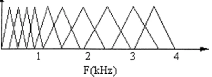
In speaker recognition systems, the Mel-frequency cepstral-coefficients (MFCC’s) are usually used as features to characterize the speech signal [1C]. Brief!}', the MFCC’s are computed by smoothing the Fourier transform spec­ trum by integrating the s])ectra.l coefficients within triangular bins arranged on

a non-linear scale called the Mel-scale shown in Figure 5.1. This scale tries to imitate the frequencj^ resolution of the human auditory system which is linear up to 1 kHz and logarithmic thereafter. In order to make the statistics of the estimated speech power spectrum approximately Gaussian, logarithmic com­ pression is applied to the energy obtained from each frequency bin. Finallj^ the Discrete Cosine Transform (DCT) is applied in order to compress the spectral information into the lower-order coefficients. Moreover, the DCT de-correlates these coefficients allowing the subsequent statistical modeling to use diagonal covariance matrices.

Figure 5.1: Triangular bins arranged on a Mel-scale for MFCC features extrac­ tion.

Gaussian Mixture Models (GMM) have been used very widely in speaker recognition applications for modeling speaker identity. Short-term (usually

20 ms) speaker-dependent feature vectors are first obtained from the speech signal, then GMM is used to model the density of these vectors. The individual Gaussian components of a GMM are shown to represent some general speaker- dependent spectral shapes that are efficient for modeling speaker identity. For speaker identification, each speaker is represented by a GMM and is referred to by his/her model.

5.2

N ew N onlinear Frequency Scale

The Mel-scale, which is approximately linear below 1 kHz and logarithmic above, is more appropriate than linear scale for speech recognition performance across frequency bands. This scale tries to imitate the frequency resolution of the human auditory system which is linear up to 1 kHz and logarithmic thereafter. However, in [17], we observed that the use of scales other than the Mel-scale may be more advantageous for speaker recognition applications.

In [24], properties of various frequency bands in the range between 0-4 kHz was investigated for accent classification. It was shown that for speech recog­ nition applications the lower range frequencies, mainly between 200-1500 Hz, have most of the relevant information. This explains the use of Mel-scale for speech recognition. While for accent classification applications, it was shown that the most relevant frequency band lies around 2 kHz. This suggests that mid-range-frequencies (1500-2500 Hz) contribute more to accent classification performance. Following these results, a new frequency axis scale was formu­ lated for accent classification [24], which is shown in Figure 5.2. Since a large number of filter banks are concentrated in the mid-range frequencies, the out­ put coefficients are better able to emphasize accent-sensitive features.

Similarly, the frequency range that is most relevant for speaker recognition is investigated in this paper. Then a scale that gives more emphasis to this frequency range is formulated.

In [24], a series of experiments were performed to investigate the accent discrimination ability of various frequency bands. We carried out similar ex­ periments to investigate the importance of different frequency bands in speaker

A ' ^ W V \ A / W

mA/\/\ \

F(kHs)

Figure 5.2: A sampling scheme for filter banks which is more sensitive to accent characteristics.

recognition. The frequenc}' axis (0-4 kHz) was divided into 16 uniformly spaced frequency bands. The energy in each frequency band was weighted with a tri­ angular window. The output of each filter bank was used as a single parameter in generating a GMM for each speaker. Figure 5.3 shows speaker identifica­ tion performance across the 16 linearly spaced frequency bands. Unlike speech recognition, the most relevant frequency band lies slightly above 2 kHz.

Figure 5.3; S])eaker identification performance based on the energy in different frequencA' bands.

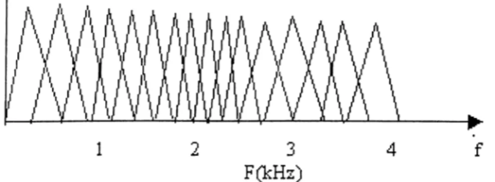
In accordance with the previous result, a new frequenc}^ axis scale is de­ rived. The scale is shown in Figure 5.4. Since a relatively large number of filters (windows) are concentrated in the midrange frequencies, the output co­ efficients are better able to emphasize speaker-dependent features. The 16 center frequencies of the filters which range between 0-4 kHz are also given in Table 5.1.

Figure 5.4: A new frequency axis division suitable for speaker recognition applications.

Filter # Center frequency (Hz) Filter # Center frequency (Hz)

1 350 9 2100 2 700 10 2220 3 1000 11 2390 4 1250 12 2600 5 1450 13 3000 6 1650 14 3300 7 1850 15 3500 8 2000 16 3700

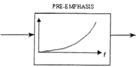
Table 5.1: Center frequencies (Hz) of triangular windows shown in Figure 5.4. Usually a ])re-ernphasis, shown in Figure 5.5, is applied to the magnitude spectrum from each speech frame. This pre-emphasis gives more importance to mid-range and high frequencies and has proven to be effective in speaker recognition.

PRE-E№HASIS

Figure 5.5: Pre-ernphasis applied to speech frames.

After the pre-emphasis and log compression, the cepstral features are com­ puted using the discrete cosine transform (DCT).

5.3

Subband D ecom position (W avelet) B ased

C om putation of Features

The wavelet analysis associated with a. corresponding decomposition filterbank is proposed in [18] to obtain a scale similar to the one derived in the previ­ ous section. The implementation of the wavelet packet transform can differ according to the application. In this case, a tree structure which uses a sin­ gle basic building block is used repeatedly until the desired decomposition is accomplished [19]- [20]. This single block, shown in Figure 5.6, divides the frequency range of the input into two half-bands.

S[n],

LPF --- 2-i --- ^ S,[n] HPF --- -- 21- --- >-SJn]

Figure 5.6: Basic block of a subband decomposition.

The pass-bands for the low-pass and high-pass filters are [O, |] and

respectively. One possible choice for these filters is the order Lagrange filters having transfer functions

(5.1) (5.2) Using subband decomposition, a frequency domain decomposition similar to Mel-scale can be obtained [18], the corresponding scale is shown in Figure 5.7. In [18], the resulting cepstral coefficients are called SUBCEP’s.

■ .1. _____L

Figure 5.7: Subband decomposition approximation to Mel-scale.

In speaker recognition within the telephone bandwidth, the frequency range 0-4 kHz is decomposed in a manner to give more emphasis to mid-range fre­ quencies between 2 and 2.75 kHz. The corresponding frequency domain de­ composition is shown in Figure 5.8.

J ____ I____ I____ I I I I . I___I___ ^___L

Figure 5.8: Frequency scale for speaker recognition using subband decomposi­ tion.

5.4

E xperim ental S tudy and C onclusions

5.4.1

D atabase D escrip tion

The experiments were carried out on the POLYCOST 250 database (vl.O). The POLYCOST database is dedicated to speaker recognition applications [26]. The main purpose behind it is to provide a common database on which speaker recognition algorithms can be compared and validated. The database was recorded from 134 subjects coming from 14 European countries. Around 10 sessions were recorded for each subject, each session contains 14 items. The recordings were made over the telephone network with an 8 kHz sampling frequenc,y. In [26], a set of baseline experiments is defined for which results should be included when presenting evaluations made on this database. Our experiments follow the set of rules defined in [26] under “text-independent speaker identification” .

5.4.2

E xperim ental R esu lts

A set of experiments was carried out to anal}'ze the performance of the pro­ posed freciuenty scale for speaker identification. The speech signal is first analyzed, and the silence periods are removed. Then the signal is divided into overlapping frames of approximately 20 ms length and a spacing of 10 ms. For each frame, 12 speech features are extracted. The experiments were done using features obtained from both methods described previousl}', i.e., cepstral features computed via Fourier analysis and wa.velet analysis (SUBCEP) using frequency sealers shown in Figure 5.4 and Figure 5.8, respectively. Table 5.1

shows the results oirtained for both methods for different frequenc}^ scales. The first column is computed using the DFT while the second column is computed using wavelet analysis.

Recognition rate using DFT analysis based cepstral features

Recognition rate using wavelet analysis based cepstral features

Mel-scale 77.8% 78.4%

Modified Mel-scale derived for accent classification

78.9% 79.5% Frequency scale derived for

speaker Identification

79.5% 80.7%

Table 5.2; Speaker identification performance for different frequency domain scales using MFCC and SUBCEP features.

The results obtained in Table II confirm that the Mel-scale is not appro­ priate for speaker recognition applications. In fact, Mel-scale performs slightly better than a uniform decomposition of the frequency domain. The frequency scale derived in [24] for accent classification performs better than the Mel- scale. This is mainly due to the fact that this scale emphasizes mid range frequencies which are important for speaker recognition. Finally, the new de­ rived frequency scale for speaker identification performs the best among the three scales. This scale emphasizes exactly the frequency bands that are most significant for speaker identity.

The experimental results also show that the use of wavelet analysis for feature extraction performs slightly better than MFCC’s which are computed using DFT. We finally conclude that the choice of the frequency domain scale should dej)end primarily on the type of application under consideration. For speaker recognition, it is shown that mid-range and some high frequency com­ ponents are more important for representing speaker identity.

C h ap ter 6

C on clu sion

In this thesis, the design of Gaussian mixture models for arbitrary densities was studied. Estimation of model parameters is one of the most important issues in GMM design. The Expectation-Maximization algorithm is widely in literature as a method for estimating these parameters. GMM parameters are usually estimated from a set of observed data. Since the density function to be estimated should be close to the histogram of the observed data in shape, the latter can be used to derive good model estimate. In this work, we proposed two new methods for estimating GMM parameters based on this approa.ch, which overcome some drawbacks of the EM algorithm.

The first method is based on least squares estimation. The least squares criterion is used to minimize an error function based on the difference between the observation data histogram and the estimated densitj^ The minimization is carried out using the Gauss-Newton optimization technique. This technique usually needs a very few number of iterations to converge. Simulations results

have shown tliat the model estimated using the proposed method is more ac­ curate than the EM based model, in the sense that the mean squared error between the estimated density and the data histogram is lower. In the opti­ mization procedure, the step size related to the perturbation vector used in the parameter update formula, has an important effect on the convergence speed and the final model error. We have provided a simple method for obtaining an estimate to the perturbation step size at each iteration of the Gauss-Newton al­ gorithm. Experimental results showed an increase in model convergence speed and accuracy when this method was applied.

Human skin color distribution modeling was used as an experimental exam­ ple to the a.pplication of the suggested method. The results showed a significant increase in the model accuracy when our method is used instead of the EM based method.

In the second method, we used the matching pursuit algorithm to decom­ pose the histogram of the observation data with a proposed set of decom­ position functions. The decomposition results in a set of weighted Gaussian functions which was used to obtain a G MM for the density function of the process under c:onsideration. This method provides a fast way to obtain GMM parameter estimates. In the application of speaker identification, the proposed method resulted in a less accurate model then the EM algorithm but the re­ quired training time was remarkably lower. Still, the matching pursuit based method further needs to be investigated for applications where speed is impor­ tant. The use of this method may be advantageous in applications like speaker adaptation.

In Chapter 5, we developed a new set of sjreech feature parameters th at are more appropriate for speaker recognition applications than the commonly used Mel-scale based features. The proposed features are based on a nonlinear divi­ sion of the freipiency scale that gives more importance of mid-range frequencies around 2 kHz. In a set of experiments on speaker identification, we found that the suggested set of features results in some increase in the identification rate.

Each of the proposed GMM parameter estimation methods has its advan­ tage. In fact, the two methods can be exploited together in one system. For ex­ ample, in an application, the model obtained b}^ the matching pursuit method can be used a good initial point for the Gauss-Newton based method. This can result in a faster convergence of the optimization procedure. Another interest­ ing application is to use the Gauss-Newton method to obtain a starting model for our process, then whenever new data comes the matching pursuit method can be used to adapt the existing model to the new data in a fast manner. The adaptation procedure can be done using a method called modeling weighting. Briefl)', what modeling weighting does is whenever there is new adaptation data the final model is calculated as a weighted sum of the original model and the model derived from the adaptation data. A smaller weight is given to the adaptation model, also a forgetting factor can be inserted with time.