Heart motion prediction based on adaptive estimation aşgorithms fo robotic-assisted beating heart surgery

(1)

HEART MOTION PREDICTION BASED ON ADAPTIVE

ESTIMATION ALGORITHMS FOR ROBOTIC-ASSISTED

BEATING HEART SURGERY

a thesis

submitted to the department of electrical and

electronics engineering

and the graduate school of engineering and science

of bilkent university

in partial fulfillment of the requirements

for the degree of

master of science

By

Eser Erdem Tuna

September, 2011

(2)

I certify that I have read this thesis and that in my opinion it is fully adequate, in scope and in quality, as a thesis for the degree of Master of Science.

Assoc. Prof. Dr. Cenk C¸ avu¸so˘glu (Co-Supervisor)

Prof. Dr. Hitay ¨Ozbay (Co-Supervisor)

Prof. Dr. ¨Omer Morg¨ul

Assist. Prof. Dr. Ulu¸c Saranlı

Approved for the Graduate School of Engineering and Science:

Prof. Dr. Levent Onural

Director of the Graduate School of Engineering and Science ii

(3)

ABSTRACT

HEART MOTION PREDICTION BASED ON ADAPTIVE

ESTIMATION ALGORITHMS FOR ROBOTIC-ASSISTED

BEATING HEART SURGERY

Eser Erdem Tuna

M.S. in Electrical and Electronics Engineering

Supervisors: Assoc. Prof. Dr. Cenk C¸ avu¸so˘glu and Prof. Dr. Hitay ¨Ozbay September, 2011

Robotic assisted beating heart surgery aims to allow surgeons to operate on a beating heart without stabilizers as if the heart is stationary. The robot actively cancels heart motion by closely following a point of interest (POI) on the heart surface—a process called Active Relative Motion Canceling (ARMC). Due to the high bandwidth of the POI motion, it is necessary to supply the controller with an estimate of the immediate future of the POI motion over a prediction horizon in order to achieve sufficient tracking accuracy. In this thesis two prediction algorithms, using an adaptive filter to generate future position estimates, are studied. In addition, the variation in heart rate on tracking performance is studied and the prediction algorithms are evaluated using a 3 degrees of freedom test-bed with prerecorded heart motion data.

Besides this, a probabilistic robotics approach is followed to model and character-ize noise of the sensor system that collects heart motion data used in this study. The generated model is employed to filter and clean the noisy measurements collected from the sensor system. Then, the filtered sensor data is used to localize POI on the heart surface accurately. Finally, estimates obtained from the adaptive predic-tion algorithms are integrated to the generated measurement model with the aim of improving the performance of the presented approach.

Keywords: Active relative motion canceling, signal estimation, medical robotics, surgical robotics, probabilistic robotics.

(4)

¨

OZET

ROBOT˙IK-DESTEKL˙I KALP AMEL˙IYATLARI ˙IC

¸ ˙IN

UYAB˙ILEN TAHM˙IN ALGOR˙ITMALARINA DAYALI

KALP HAREKET˙I TAHM˙IN˙I

Eser Erdem Tuna

Elektrik ve Elektronik M¨uhendisli˘gi, Y¨uksek Lisans

Tez Yöneticileri: Do¸c. Dr. Cenk Ç avu¸so˘glu ve Prof. Dr. Hitay Özbay Eylül, 2011

Robotik destekli atan kalp ameliyatı, cerrahlara atan kalp üzerinde dengeliyiciler olmadan, kalp sabitmi¸s¸cesine ¸cal¸smaları i¸cin olanak sa˘glamaktadır. Robot, kalp yüzeyindeki bir ilgi noktasını etkin bir bi¸cimde, yakından takip ederek kalp hareke-tini iptal eder. Bu yönteme “Etkin Göreceli Hareket Önleyici (EGH Ö)” denilmek-tedir. ˙Ilgi noktasının yüksek bant geni¸sli˘gindeki hareketi nedeniyle, yeterli takip do˘grulu˘gunu sa˘glamak i¸cin, denetleyiciye ilgi noktasının hareketinin bir tahmin ufku boyunca yakın bir tahminini sa˘glamak gerekmektedir. Bu tezde, gelecekteki konum tahminini olu¸sturmak i¸cin uyabilen süzge¸c kullanan iki tahmin algoritması ¸calı¸sılmı¸stır. Buna ek olarak, kalp hızı de˘gi¸siminin takip performansı üzerine etkisi ¸calı¸sıldı ve tahmin algoritmaları 3 serbestlik derecesi olan bir sınama ortamı kul-lanılarak önceden kaydedilmi¸s kalp hareketi verileri ile de˘gerlendirildi.

Bunların yanında, bu ¸calı¸smada kullanılan kalp hareket verilerini toplayan sezici sistemin gürültüsünü tanımlamak i¸cin olasılıksal bir robotik yakla¸sım takip edildi. Olu¸sturulan model, sezici sistemden toplanan gürültülü öl¸cümleri süzmek ve temiz-lemek i¸cin istihdam edildi. Daha sonra, süzülmü¸s sezici öl¸cümler, ilgi noktasının kalp yüzeyindeki yerinin do˘gru bir ¸sekilde belirlenmesi i¸cin kullanıldı. Son olarak, uyabilen tahmin algoritmalarından elde edilen tahminler, sunulan yakla¸sımın performansını arttırmak amacıyla olu¸sturulan öl¸cüm modeline dahil edildi.

Anahtar sözcükler : Etkin göreceli hareket önleyici, sinyal tahmini, tıbbi robotik, cerrahi robotik, olasılıksal robotik.

(5)

Acknowledgement

First, I would like to express my deep gratitude to Dr. Cenk C¸ avu¸so˘glu for letting me involved in this research and giving me the opportunity of being a part of the MeRCIS lab. His endless support and guidance always kept me motivated and gave me hope throughout my study. I really appreciate his encouragement and steadfastness which influenced me and helped me to complete this work.

Especially, I am grateful to Dr. Hitay ¨Ozbay for his invaluable advice during these years. I would like to thank him for teaching me to think broadly and innovatively and leading me to the control systems field. His considerate and understanding personality as a mentor helped me to make the right choices in my career as a graduate student.

I am also thankful to Dr. ¨Omer Morg¨ul and Dr. Ulu¸c Saranlı for showing keen interest to the subject matter and accepting to read and review this thesis.

A special thanks goes to Dr. ¨Ozkan Bebek for all his help and support during the completion of this study. His enthusiasm in the surgical robotics, his inspiring ideas and our enlightening discussions provide significant contributions to the presented study which have been put into use in this thesis.

I am also appreciative of the generous support from Bilkent University, Depart-ment of Electrical and Electronics Engineering.

Last but not least, I am indebted to my family for their love and for believing in me.

(6)

Dedeme ve anneanneme

(7)

List of Figures

1.1 System Concept for Robotic Telesurgical System for Off-Pump CABG

Surgery . . . 2

1.2 Proposed Control Architecture for Active Relative Motion Canceling 4 1.3 Piezoelectric Crystals . . . 6

2.1 Experimental Setup for Measurement of Heart Motion . . . 13

2.2 Power Spectral Density of the Motion of the Point of Interest . . . 15

2.3 Variation of Heart Rate in the Heart Motion . . . 16

3.1 A Schematic of the Prediction Problem . . . 19

3.2 Concept of the Adaptive Predictor . . . 24

3.3 Generation of the Horizon by the Adaptive Filter . . . 28

4.1 Zero Configuration of the PHANToM Manipulator . . . 33

4.2 Tracking Results for Constant Heart Rate Heart Motion Data . . . . 38 xi

(12)

LIST OF FIGURES xii

4.3 Tracking Results for Varying Heart Rate Heart Motion Data . . . 39 4.4 RMSE of One-Step Predictions in the Presence of Varying

Measure-ment Noise . . . 43 4.5 RMSE of One-Step Predictions in the Presence of Varying Heart Rate 44

5.1 Harmonic Approximation of the Sensor Data . . . 54 5.2 Sonomicrometry Sensor Model . . . 57 5.3 Sonomicrometry Base Plate, 3D Crystal Position Coordinates and

Dis-tances Between Crystals . . . 58 5.4 Normalized Histogram of the Error Between Sensor Measurements and

Actual Data. . . 61 5.5 Density Distribution of the Generated Noise Model for Heart Motion

Data . . . 62

6.1 The 3D Position Coordinates of the 6th _{Crystal . . . .} ₇₅

6.2 Density Distribution of the Generated Noise Model for Sonomicrom-etry Sensor Data . . . 76 6.3 Filtered Sensor Data by EKF with Harmonic Motion Model . . . 78 6.4 The 3D Position Coordinates of the Moving Crystal Localized by EKF

Harmonic Motion Model . . . 79 6.5 z-Coordinate of the 3D Position of POI . . . 80 6.6 Filtered Heart Motion Data by EKF with Harmonic Motion Model . 82

(13)

LIST OF FIGURES xiii

6.7 The 3D Position Coordinates of the Moving Crystal Localized by EKF Harmonic Motion Model . . . 83

(14)

List of Tables

4.1 Simulation Results for End-Effector Tracking . . . 35 4.2 Experiment Results for End-Effector Tracking . . . 36 4.3 Experimental Results for End-Effector Tracking: RMS End-Effector

and Maximum Position Errors for the Controller with EKF Predictor 41

6.1 Simulation Results for a 70 sec long Sonomicrometer Data: RMSE for the Probabilistic Localization Algorithms. . . 77 6.2 Simulation Results for a 60 sec long Constant Heart Rate Motion

Data: RMSE for the Probabilistic Localization Algorithms. . . 81 6.3 Simulation Results for a 60 sec long Constant Heart Rate Motion

Data: RMSE for the Probabilistic Localization Algorithms. . . 85

(15)

Chapter 1 Introduction

1.1 Coronary Artery Bypass Graft Surgery

Coronary artery bypass graft (CABG) surgery requires surgeons to operate on blood vessels that move with high bandwidth. This rapid motion of heart makes it diffi-cult to track these arteries by hand effectively [1]. Contemporary techniques either stop the heart and use a cardio-pulmonary bypass machine or passively restrain the beating heart with stabilizers in order to cancel the biological motion of heart dur-ing CABG surgery. However usdur-ing on-pump CABG surgery might expose patient to suffer from long term cognitive loss due to complications that can occur during or after the surgeries as a consequence of stopping the heart [2]. Off-pump CABG surgery with stabilizers is limited to the front surface of the heart and significant residual motion is observed during stabilization [3].

(16)

CHAPTER 1. INTRODUCTION 2

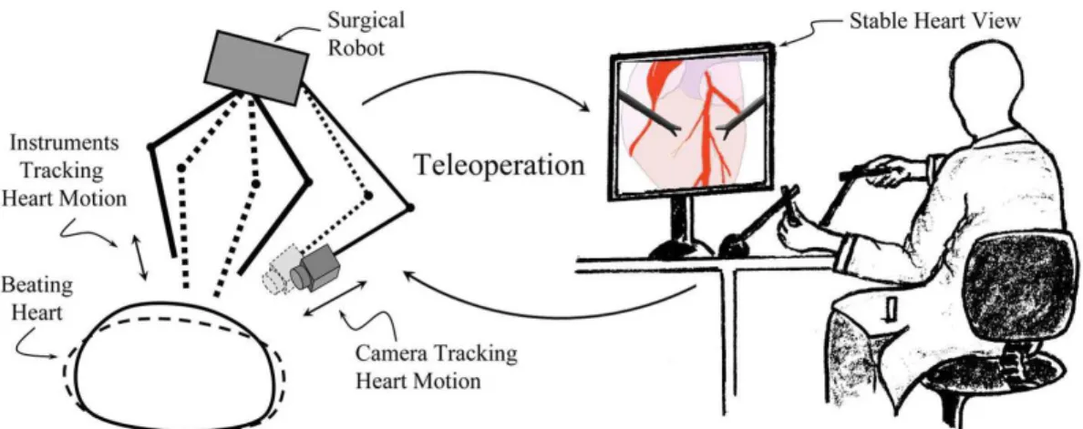
Figure 1.1: System Concept for Robotic Telesurgical System for Off-Pump CABG Surgery with Active Relative Motion Canceling (ARMC). Left: Surgical instruments and camera mounted on a robot actively tracking heart motion.

1.2 Robotic-Assisted Beating Heart Surgery

Robotic-assisted beating heart surgery emerges as a novel technology, which replaces the conventional surgical tools with robotic instruments. Figure 1.1 illustrates the proposed robotic assisted surgical system. In this system, a camera which is mounted on a robotic arm follows the heart motion. A surgical robot, which moves simulta-neously with the heart, is used to track and cancel the relative three dimensional heart motion. By this way, it allows surgeon to experience the surgical site via stabi-lized views. Surgeon directly controls the surgical instruments through teleoperation and surgical instruments track heart motion and cancel the relative motion between heart and the instruments. Thus, the surgeon operates on heart as if it is station-ary. This approach is called “Active Relative Motion Canceling (ARMC)”. This would eliminate the need for stopping the heart and the use of cardio pulmonary bypass machine (the pump). Hence, robotic-assisted CABG surgery will prevent the occurrence of risks due to on-pump CABG surgery. It differs from the traditional off-pump CABG surgery with stabilizers since in the proposed robotic-assisted sur-gical system, heart motion is canceled with motion compensation. In contrast in the

(17)

traditional off-pump CABG surgery, heart is passively constrained with mechanical stabilizers [4].

1.3 Motion Estimation Algorithms for Model

Based Active Relative Motion Canceling

Al-gorithms

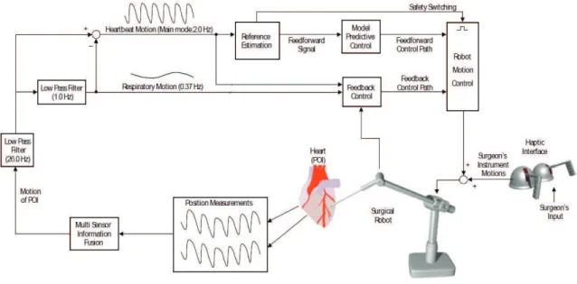
In CABG surgery, surgeon is required to operate on small blood vessels which move very rapidly. Their diameters vary from 0.5 to 2 mm and they have a quasiperiodic motion at the rates of 1 to 2 Hz. RMS tracking error for the position of a point of interest (POI) on the heart surface has to be in the order of 100-250 µm to perform precise operations on these vessels. The robotic tools need to track and manipulate a fast moving target with very high precision [5]. Causal error feedback control alone is not able to reduce the tracking error sufficiently such that surgery can be done on blood vessels on the heart surface. A predictive controller which implements a receding horizon model predictive control (RHMPC) in the feedforward path was found to be necessary [6, 7]. The proposed control architecture for designing motion estimation algorithm for ARMC on the beating heart surgery is shown in Figure 1.2 In the Model Based ARMC Algorithm architecture, the control algorithm fuses information from mechanical motion sensors which measure the heart motion. Mo-tion of the point of interest (POI) has two dominant modes of moMo-tion, lung moMo-tion and heartbeat motion. These two modes are separated using proper filters. Lung motion has significantly lower frequency, and it can be canceled by a simple causal feedback controller. On the other hand, heartbeat motion has more demanding re-quirements in terms of the bandwidth of the motion that needs to be tracked. Thus a feedforward controller is required to cancel heartbeat motion.

(18)

Figure 1.2: Proposed control architecture for designing Intelligent Control Algo-rithms for Active Relative Motion Cancelling on the beating heart surgery.

The confidence level reported by the heart motion model will be used to adap-tively weight the amount of feedforward and feedback components used in the final control signal. This confidence level will also be used as a safety switching signal to turn off the feedforward component of the controller if an arrhythmia is detected, and switch to a further fail-safe mode if necessary. These safety features will be an important component of the final system.

The primary goal of this research is to improve the tracking performance of a sur-gical robot prototype as proof of concept that motion cancelation can be achieved. To this end, the tracking performance research has primarily been focused on devel-oping estimation methods for use with a RHMPC. Such a predictive controller needs an estimate of the future motion of the POI on the heart surface. The estimate needs to be of a finite duration into the future, referred to as the prediction horizon.

(19)

In this thesis, heart motion prediction methods based on adaptive filtering tech-niques are studied. The implementations parametrize a linear system to predict the motion of the POI and rely on recursive least square adaptive filter algorithms. The presented methods differ as the first one assumes a linear system relation between the consecutive samples in the prediction horizon whereas the second method performs this parametrization independently for each point throughout the horizon. The ef-fectiveness and feasibility of these algorithms are studied by simulations and on a 3-degree-of-freedom (DOF) hardware with constant and varying heart rate data.

The presented one step adaptive filter and the generalized adaptive filter are initially described by Franke et al. in [8] and [9] respectively. During the course of this research, these two algorithms are exhaustively and extensively studied. The bugs and errors in these predictors are fixed and the generalized predictor is completely re-implemented. As a result of this effort, the prediction performance of the algorithms and eventually the tracking performance of the intelligent control algorithms are significantly improved. These two algorithms are explained for the completion of the work and the results presented in this thesis.

1.4 A Probabilistic Robotics Approach for

Sens-ing

A sensor that is in continuous contact with tissue is necessary for satisfactory track-ing. The continuous contact sensor used in measuring the heart motion in the current literature is a Sonomicrometry system manufactured by Sonometrics Inc. (London, Ontario, Canada). A Sonomicrometer measures the distances within the soft tissue via ultrasound signals. A set of small piezoelectric crystals attached to the tissue are used to transmit and receive short pulses of ultrasound signal, and the time of flight of the sound wave as it travels between the transmitting and receiving crystals are

(20)

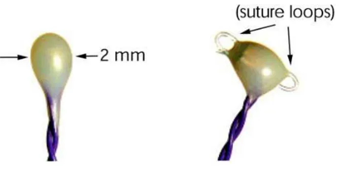
Figure 1.3: Piezoelectric crystals (courtesy of Sonometrics Corporation). Left: Stan-dard piezoelectric crystal in 2 mm diameter that were used on the base plate. Right: Piezoelectric crystal with suture loops embedded to the crystal head. Loops are used to suture the crystal onto muscle.

measured (see Figure 1.3) [10].

The Sonomicrometric position sensor has been the sensor of choice in the earlier studies of this research, but obtaining precise position measurements is essential in closed loop control for tracking the beating heart. Despite sonomicrometric sensors are very accurate, they contain noise from ultrasound echoes. [4].

It is crucial to provide good quality of heart motion data to intelligent control algorithms to make sure that these algorithms follows and cancels motion of POI on heart surface accurately. In this part of the research, a probabilistic robotics approach is followed to model the noise of the Sonomicrometry sensor system and a Bayes estimator is used to filter and clean the noisy measurements collected from the Sonomicrometry sensor system. Then the POI on the heart surface is localized using this filtered measurements.

The main reason for following a probabilistic robotic approach is to represent uncertainty in the sensor system explicitly, using the calculus of probability theory. In other words, instead of relying on a single hypothesis as to what might be the

(21)

exact effect of the ultrasound echoes on measurements, the applied probabilistic algorithms represent information by probability distributions over a whole space of possible hypotheses.

1.5 Contributions

This thesis presents two heart motion prediction methods based on adaptive filtering techniques. The presented methods differ as the first one assumes a linear system relation between the consecutive samples in the prediction horizon whereas the sec-ond method performs this parametrization independently for each point throughout the horizon.

Although, the presented one step adaptive filter and the generalized adaptive filter are initially described by Franke et al. in [8] and [9] respectively, the bugs and errors in these predictors are completely fixed and the generalized predictor is completely re-implemented.

In the literature these predictors are tested with very limited and short duration of data. During the course of this research, these two algorithms are exhaustively and extensively studied with a wide range of different heart motion data. Predictors are tested with both constant and varying heart rate motion data. This is the first study that uses real varying heart rate data to perform heart motion tracking. As a result of this effort, the prediction performance of the algorithms and eventually the tracking performance of the intelligent control algorithms are significantly improved. With the presented algorithms, the estimation of future POI motion is no longer the bottleneck in the heartbeat motion tracking since the necessary amount of RMS tracking error for the POI on the heart surface is achieved to perform precise oper-ations.

(22)

In this work, an effective probabilistic robotics approach is applied to model and characterize noise of the sensor system that is used to collect heart motion data used in this study. The applied model completely covers the noise of the sensor system and effectively filters the noisy measurements. In an in-vivo heart tracking experiment, this preliminary approach will provide an online filtering mechanism for the noisy sensor measurements and localize point-of-interest on the heart surface accurately.

1.6 Thesis Outline

The rest of this thesis is organized as follows. Related work and analysis of the experimental heart motion data are given in Chapter 2. Problem formulation, the prediction methods and how the methods differ from each other to create estima-tions throughout the prediction horizon are explained in Chapter 3. Implementation details are also addressed in this chapter. In Chapter 4 simulation and experimental results are given. Chapter 5 describes the probabilistic approach that is applied the model noise in the sensor system and explains two different localization algorithms that are used to filter and clean noisy sensor measurements in order to accurately localize the Point-of-Interest(POI) on heart. The results of the localization algo-rithms are given in Chapter 6. Finally, the discussion and conclusions are presented in Chapter 7.

(23)

Chapter 2 Background

2.1 Related Works in Literature

This thesis is concerned with estimating the prediction horizon for RHMPC–a control scheme that relies on the estimate of the prediction horizon as a reference signal. There has already been several proposed ways to estimate motion of a POI on the heart surface.

Nakamura et al. [11] performed experiments to track the heart motion with a 4-DOF robot using a vision system to measure heart motion. The tracking error due to the camera feedback system was relatively large (error on the order of few millimeters in the normal direction) to perform beating heart surgery. There are also other studies in the literature on measuring heart motion. Thakor et al. [12] used a laser range finder system to measure one-dimensional motion of a rat’s heart. Groeger et al. [13] used a two-camera computer vision system to measure local motion of heart and performed analysis of measured trajectories, and Koransky et al. [14] studied the stabilization of coronary artery motion afforded by passive cardiac stabilizers using

(24)

CHAPTER 2. BACKGROUND 10

3-D digital sonomicrometer. Richa et al. developed a tracking algorithm for the heart surface based on a thin-plate spline deformable model [15], and an illumination compensation algorithm which can cope with arbitrary illumination changes on the heart [16].

Ortmaier et al. [17] used Takens Theorem to develop a robust prediction algo-rithm, anticipating periods of lost data when a tool obscured the visual tracking system. Estimates were generated from a linear combination of embedding vectors of previous heart data. The weights were chosen such that better estimating vectors are weighted more heavily. The algorithm had a global prediction technique that correlated ECG signals to heart motion. It was able to estimate the system behavior when visual contact of the landmark was lost for some period of time.

Ginhoux et al. [7] separated breathing motion from heart motion in the prediction algorithm. The breathing motion was treated as perfectly periodic, since the patient would be on a breathing machine. The heart motion was predicted by estimating the fundamental frequency, as well as the amplitude and phase of the first 5 harmonics. This prediction was used to estimate disturbance so that the controller could correct for it.

Rotella [6] used the previous cycle of heart motion data as an estimate of future behavior. This lead to problems since the POI motion was not perfectly periodic. Bebek and Cavusoglu [4] improved upon this prediction scheme by synchronizing heart periods using ECG data and separated heart and breathing motion, predicting only heart motion. Bebek noted that the prediction method still could be improved. Bader et al. [18] presented a model-based approach for reconstructing the position of any arbitrary POI and for predicting the heart’s surface motion in the intervention area. They model the motion of a POI on heart surface by means a pulsating membrane model. The membrane motion is described by means of a system of coupled linear partial differential equations (PDEs) and obtained a bank of lumped

(25)

systems after spatial discretization of the PDE solution space by the Finite Spectral Element Method. A Kalman filter is employed to estimate the state of the lumped systems by incorporating noisy measurements of the heart surface.

Yuen et al. [19] developed a 1-DOF ultrasound-guided motion compensation sys-tem for cardiac surgery. The surgical syssys-tem integrates 3D ultrasound imaging and a robotic instrument with a predictive controller that compensates for the 50-100 ms imaging and image processing delays to ensure good tracking performance. Yuen et al. [20] used Extended Kalman Filter (EKF) algorithm to predict the future position of mitral valve annulus motion. The EKF filter is used to feed-forward the trajectory of a cardiac target in order to compensate time delays occurred due to the acquisition of motion data by the 3D ultrasound imaging. They tested the performance of EKF in prediction and tracking in the presence of high measurement noise and heart rate variability. They reported RMS synchronization errors of 1.5 mm for trajectories derived from clinical heart rate variability data.

This thesis introduces new estimation algorithms into the controller described in the earlier work of Rotella [6] and Bebek and Cavusoglu [4]. New prediction technique using adaptive filters are proposed and used in place of the prediction algorithm of Bebek and Cavusoglu [4]. Since the new predictors are parameterized by a least squares algorithm, the predictors are inherently robust to noise. The predictors only use observations close to and including the present making it less susceptible to differences between heart periods than the algorithm of Bebek and Cavusoglu [4]. Where as Ginhoux et al [7] formulated prediction for periodic POI motion, no assumptions are made towards periodicity of the system a priori, rather the predictors are unconstrained so that they can best mimic the motion of the POI. The adaptive prediction algorithms presented in this thesis tested with constant and varying heart rate motion data. This is the first study that uses real varying heart rate data to perform heart motion tracking.

(26)

In addition, tracking and prediction performance of the adaptive predictors pre-sented in this thesis and the EKF predictor used in the study of Yuen et al. [20] are compared.

2.2 Analysis of Heart Data

In this section of the thesis, the experimentally collected varying heart rate motion data, which are used in this study, are described. Data were collected from three calves and all the study is performed with on benchtop with these pre-recorded data. First the collection of heart motion data will be explained. Then the analysis of varying heart rate motion data is presented.

2.2.1 Experimental Setup for Measurement of Heart Motion

The prerecorded data used in this study was collected using a Sonomicrometry sys-tem (Sonometrics Inc., Ontario, Canada). The Sonomicrometry syssys-tem has also been the sensor of choice in our previous work for measuring heart motion for robotic ARMC [4]. A Sonomicrometer measures the distances within the soft tissue via ultrasound signals. A set of small piezoelectric crystals attached to the tissue are used to transmit and receive short pulses of ultrasound signal, and the “time of flight” of the sound wave as it travels between the transmitting and receiving crys-tals are measured. Using these data, the 3-D configuration of all the cryscrys-tals can be calculated [10]. Absolute accuracy of the Sonomicrometry system is 250 µm (approximately 1_/₄ _{wavelength of the ultrasound) [21].}

In the experimental set-up one crystal of the Sonomicrometry system was sutured on the heart . While collecting measurements, this crystal on the heart was placed in two different locations. The first location, which is referred to as ‘Top’ in the rest of

(27)

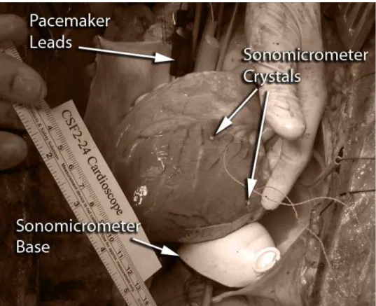
Figure 2.1: Experimental setup for measurement of heart motion. Two Sonomicrom-eter crystals that are sutured on the anterior and posterior surfaces of the heart are used for data collection. Pacemaker leads and Sonomicrometer base are also visible in the image.

the thesis, is located on the front surface. Specifically, the Sonomicrometry crystal was placed at 1 cm laterally from the left anterior descending coronary artery and 8 cm cranially from the LV apex. The second location, which is referred to as ‘Side’, is the location on the side surface of the heart. Specifically, in this case, the crystal was placed at 5 cm laterally from the left anterior descending coronary artery and 10 cm cranially from the LV apex. Five other crystals were asymmetrically mounted on a rigid plastic base of diameter 60 mm, on a circle of diameter 50 mm, forming a reference coordinate frame. This rigid plastic sensor base is placed in a rubber latex

(28)

balloon which is filled with a %9.5 glycerine solution. The reason of using such a set-up is to ensure a continuous line of sight between the base crystals and the crystal on the heart surface through a liquid medium for proper operation of Sonomicrometry sensor system. Figure 2.1 shows the experimental setup for measurement of heart motion. The Sonomicrometer crystals that are sutured on the heart can be seen from the figure. The pacemaker leads that are used to change the heart rate and the Sonomicrometer base are also visible.

Data were processed offline using the proprietary software provided with the system to calculate the 3-D motion of the POI. The only filtering performed on the data produced by the Sonomicrometry system was the (very limited) removal of the outliers, which occasionally occur as a result of ultrasound echoing effects. Although the Sonomicrometry system can operate at 2 kHz sampling rate for measuring the location of the POI crystal relative to the fixed base, in our test experiments, we have collected data at sampling rates of 257 Hz and 404 Hz in order to collect redundant measurements.

2.2.2 Analysis of Varying Heart Rate Motion Data

The motion of the heart surface is quasi-periodic in nature. The motion of the POI on the heart is primarily the superposition of two effects: motion due to the heart beating and motion due to breathing. Each of these signals closely resemble periodic signals.

In practice, the statistics of heart motion is likely to change during surgery. Such a change will result in variations in the underlying dynamics of the POI’s motion. In order to explore the effects of these slow variations on the tracking performance and investigate how the adaptive algorithms will adjust to these changes, two distinct types of experimentally collected heart data is used in this study. The first type

(29)

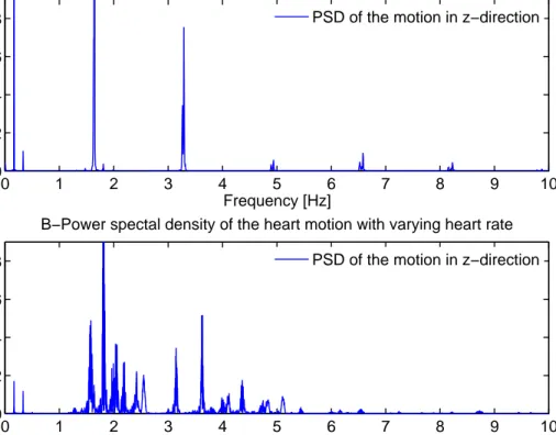
CHAPTER 2. BACKGROUND 15 0 1 2 3 4 5 6 7 8 9 10 0 2 4 6 8 Frequency [Hz] PSD [linear units]

A−Power spectal density of the heart motion with constant heart rate

0 1 2 3 4 5 6 7 8 9 10 0 2 4 6 8 Frequency [Hz] PSD [linear units]

B−Power spectal density of the heart motion with varying heart rate PSD of the motion in z−direction PSD of the motion in z−direction

Figure 2.2: Power Spectral Density (PSD) of the heart motion in the z direction. (A) PSD of heart motion with constant heart rate. Tall, narrow peaks with the absence of intermittent frequencies indicate largely periodic motion of the heart. (B) PSD of heart motion with varying heart rate.

includes constant heart rate data whereas the second type includes varying heart rate data. From each calf a duration of 736-s, 472-s and 340-s of data are processed and used in this study.

Fourier analysis of the heart signal data with constant heart rate reveals how this periodic nature is prevalent (see Figure 2.2-A). The first peak corresponds to lung motion, which has the lower frequency with a fundamental period of approximately

(30)

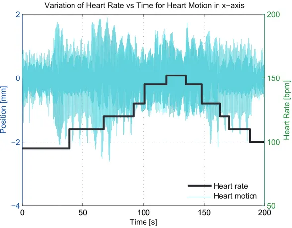
CHAPTER 2. BACKGROUND 16 0 50 100 150 200 −4 −2 0 2 Po si ti o n [ mm] Time [s]

Variation of Heart Rate vs Time for Heart Motion in x−axis

0 50 100 150 20050 100 150 200 H e a rt R a te [ b p m] Heart rate Heart motion

Figure 2.3: Variation of heart rate in the heart motion in x-direction.

0.17 Hz with first harmonic at 0.33 Hz is appearing significant. The heart motion it-self has a fundamental frequency of 1.66 Hz, corresponding to 100 bpm, with the first four harmonics clearly visible in the figure. The peak displacement of the POI from its mean location was 8.39 mm, with a root-mean-square (RMS) value of 3.55 mm. The sharpness of these peaks indicate that the harmonics decay very little in time, meaning that the overall motion of the POI is similar to a superposition of periodic signals.

In order to change the heart rate, an artificial pacemaker is employed which uses electrical impulses to regulate heart rate, generated by electrodes contacting the

(31)

heart muscles. Initially heart is allowed to beat 40 seconds at 95 bpm. Then, the heart rate is gradually increased from 95 bpm to 152 bpm by approximately 10 bpm steps and then decreased in the same way, where heart is allowed to beat for at an average 15 seconds at a particular heart rate. Figure 2.3 shows the variation in heart rate with respect to time for the heart motion in x-direction. In the Fourier analysis of varying heart rate data, Figure 2.2-B, the first observable dominant mode at 0.17 Hz corresponds the breathing motion, similar to constant heart rate data, with a significant first harmonic at 0.33 Hz. The remainder of motion which is due to the beating of heart shows the fundamental frequencies of heart motion for different heart rates. The peaks at 1.58 Hz, 1.81 Hz, 2.03 Hz, 2.18 Hz, 2.42 Hz and 2.54 Hz correspond to heart rate of 95 bpm, 110 bpm, 120 bpm, 130 bpm, 145 bpm and 152 bpm, respectively. The peak displacement of the POI from its mean location was 7.43 mm, with a RMS value of 3.38 mm.

(32)

Chapter 3 Problem Definition and Methods

3.1 Problem Formulation

The control algorithm establishes the most essential part of the robotic tools for tracking heart motion during CABG surgery. Rapid motion of heart possesses de-manding requirements on the control architecture in terms of the bandwidth of the motion that needs to be tracked. This necessity resulted in utilizing a feedforward algorithm in the control architecture in order to cancel high frequency components of heartbeat motion. In this study RHMPC (originally developed in [4]) was used as the feedforward control algorithm, requiring an estimate of the immediate future of the POI on the heart surface. If the feedforward controller has high enough pre-cision to perform the necessary tracking, then the tracking problem can be reduced to predicting the estimated reference signal effectively [4].

The following notion will be used for formulating the motion estimation problem. Let zi represent an observation at time i. In this case, zi is a three dimensional

column vector representing the location of the POI in Cartesian coordinates. At a 18

(33)

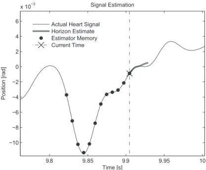
CHAPTER 3. PROBLEM DEFINITION AND METHODS 19 9.8 9.85 9.9 9.95 10 −10 −8 −6 −4 −2 0 2 4 6 x 10−3 Time [s] Position [rad] Signal Estimation

Actual Heart Signal Horizon Estimate Estimator Memory Current Time

Figure 3.1: A schematic of the prediction problem. The circles represent past ob-servations, now in memory, the ‘X’ is the current observation, and the short curve originating from there is the horizon estimate. The predictor takes the past obser-vations and produces the horizon estimate from past obserobser-vations.

given time step n, the observation zn indicates the current 3D position of the heart.

Then, the observation zn−1 represents the previous position of heart at the time n;

and the older observations will be referenced by decreasing subscript index, e.g., z_n−5 is the observation from five samples ago. In a similar fashion, zn+1 represents the

next observation at time n. Yet, this observation has not occurred, and will not be known until it becomes the present value. The estimate for the next observation at time n is introduced as ˆzn+1.

Using this notation, the prediction problem can be posed as follows: Given the N-dimensional vector of known samples leading up to time n, [zn, zn−1, . . . , zn−N+1]T,

find the best estimate of the M-dimensional horizon, [zn+1, zn+2, . . . , zn+M]T.

(34)

CHAPTER 3. PROBLEM DEFINITION AND METHODS 20

to be the one that minimizes the square of the estimation error, where the estimation error is the difference between the prediction and the observed value at that time. Once a method is established to predict the next observations, a sequence of future observations can be estimated. However, heart dynamics are nonlinear, which makes it quite challenging to parameterize a valid heart model in order to generate future predictions of POI from known samples.

Two adaptive filter based motion estimation algorithms are presented in this thesis to estimate reference signal, namely one step adaptive filter based motion estimation algorithm and a generalized adaptive filter based motion estimation al-gorithm. These two methods formulate and then parameterize the model of heart motion differently as described in the following two sections, Section 3.2 and Section 3.3.

3.2 One Step Motion Estimation Algorithm

An Nth _{order predictor has memory of past N − 1 observations together with}

ac-cessing to current observation. It generates the next expected observation in the prediction horizon based on these N observations. In order to generate the next fu-ture observation, what was just estimated is evaluated as if it was actually observed in the current time step and is added to the set of observations. Then the next value in the horizon is the next prediction that is obtained from this set. Proceeding in a similar fashion, any number of future estimates can be generated recursively till all the predictions for the horizon have been made.

In order to generate predictions in this way, the one step prediction function must be known. The motion of the POI interest is a continuous-time dynamic system, which is nonlinear as mentioned in the previous section. To establish a method for predicting future positions of POI, an equivalent discrete-time system has to be

(35)

used. Yet, neither the state space nor the dimension of the heart is obvious. So to simplify prediction method, a finite and low order state vector must be employed in the heart model. The state transition function for this approximate heart model is also nonlinear due to nonlinear dynamics of heart motion, which makes it difficult to parameterize.

The Fourier analysis of the heart signal data, presented in Section 2.2, reveals the quasiperiodic nature of the heart motion (see Figure 2.2-A). It shows that the heart position signal is composed of a main mode and additional harmonic where the motion is subject to small disturbance. This nature of heart motion allows the nonlinear state transition function to be approximated as linear by the following intuition.

The sharpness of the peaks of significant harmonics indicate that the harmonics decay very little in time, meaning that the overall motion of the POI is similar to a superposition of periodic signals. A linear system can easily be constructed that has a frequency response that mimics the heart signal’s Fourier representation. The transient response would then resemble the observed heart data. Thus, given the current state of the actual heart signal as initial values for the system, the transient response would follow the actual heart motion−giving a prediction.

Finally, if the state was formulated as a stacked vector of past observations, then the determination of the initial state would be trivial. A linear system of the above specifications would meet the requirements for the heart model transition function. However, the model would still need to be parameterized in a way to statistically minimize the error of the prediction.

(36)

3.2.1 Model of Heart Motion

The heart position data consists of 3-dimensional vectors representing position. These vector samples are assumed to be generated from a vector autoregressive model (VAR). A VAR process has multiple output signals which are correlated with each other. The model is given by following equation [22]:

~zk= N

X

i=1

Ai~zk−i+ ~γk (3.1)

In this case, it is an Nth _{order VAR model. Each observation is given by a weighted}

sum of past observations, and is perturbed by noise given by ~γk. Noise vector ~γk is

assumed to be zero mean white noise. Since the linear combination of past obser-vations account for correlation between obserobser-vations, for any two noise vectors ~γk

and ~γi, ~γk is uncorrelated with ~γi for i 6= k. Since the noise vector is assumed to

be white, it is not useful when generating predictions of future values. Therefore, when parameterizing the equation for the purpose of prediction, only the weighting matrices need to be estimated.

The VAR model given in (3.1) can be reformulated in state space canonical form as

~

Xk= Φ ~Xk−i+ Γ~vk

~σk = C ~Xk

(3.2) This system can be reformulated using an arbitrary state vector, however a stacked vector of past observations simplifies the determination of the initial state, parametrization of the state transition matrix Φ, and generation of the prediction

(37)

horizon. In this case, Φ is in canonical form and can be written as:

Φ =        A1 A2 · · · AN I 0 · · · 0 0 I ... .. . . .. 0        (3.3)

Future observations of the system are given by solving the state space solution at time n. In order to find the expected trajectory, we take the expectation of (3.2) and find that the solution takes the form

E{zn+k} = CΦkX~n (3.4)

where the above formula gives the horizon estimate made at time n for a value k steps into the future. Note that since Φk _{is only computed for k < M, where M}

is the horizon length, Φk _{always remains finite. Therefore, stability of Φ is not a}

concern. Since ~v is unknown, but its expected value is zero by construction, it does not appear in the solution to the expected trajectory.

3.2.2 Adaptive Filter

The adaptive predictor consists of two principle parts: a linear filter and an adap-tion algorithm (see Figure 3.2). The input-output relaadap-tion of the adaptive filter is determined by the linear filter. The adaptive filter’s response is the response of the linear filter to the system’s input. In this case, the linear filter will be a transver-sal filter. The adaptive algorithm changes the filter’s weights in order to make the filter’s output match the desired response in a statistical sense. The adaptive algo-rithm changes the filter’s weights, so the filter is in fact not linear time-invariant. However, when the adaptive filter is adapting to a stationary signal, it will converge

(38)

D

--+ Estimate Observation Weights Filter Adaptive Algortithm

Figure 3.2: Adaptive predictor concept; the adaptive filter is arranged to minimize the error between the estimate for the current observation, calculated in the last iteration, and the actual observed value. In this way, the weights of the filter are statistically optimized to estimate one step ahead.

to a steady state, after which point it can be treated as being linear time-invariant. If the adaptive algorithm is able to forget the past, just as it was able to converge to a stationary signal, it can track a signal with changing statistics [23]. In the special case that the statistics change slowly relative to the algorithm’s ability to adapt, then the filter can track the ideal time-varying solution. Further, if the statistics change slowly relative to the length of the prediction horizon as well as the length of the state vector, then the adaptive filter can be considered to be locally linear time-invariant. The two afore mentioned conditions are the case with modeling the heart motion during most normal situations.

The adaption algorithm uses an exponential window to weight past observations so that more recent observations carry more weight. The exponential window was chosen because it can easily be implemented recursively. Due to this windowing, the adaptive predictor is able to track the heart signal even if the statistics of the heart signal change slowly with time.

(39)

3.2.3 Parametrization

Traditional system identification problems using adaptive filters arrange the filter such that the input to the filter is the system’s input and the desired response is the system’s desired response. In this way, the filter converges towards an approximation of the system’s input-output relation. However, (Equation 3.2) is driven by white noise input vector ~v. This input is unknown and unable to be predicted for future observations. Thus, deriving an input-output relationship for the heart motion would be impractical. Instead, the adaptive filter is arranged as a one-step predictor. The desired response is the heart position’s current observation and the input to the adaptive filter is the previous heart observations. The adaptive filter adjusts its filter weights such that it generates the statistically best estimate for the next observation, given only the current and past observations.

In order to generate the predictions, the coefficient matrices, Ai, from (3.1),

equiv-alently, the matrix Φ from (3.2) need to be estimated. The state transition matrix, Φ, is in controllable canonical form, so estimating Ai is sufficient to parameterize the

estimated state transition matrix, denoted ˆΦ. As can be seen from (3.1), the matrices Ai correspond to tap weights in a transversal filter. In a one-step predictor, when

it has converged to a solution, its filter weights are precisely the matrices needed to parameterize ˆΦ. In this way the adaptive algorithm estimates the matrix ˆΦ.

3.2.4 Recursive Least Squares

Recursive least squares (RLS) was chosen as the adaptation algorithm to update the filter weights. RLS is a method that updates a least squares solution when a new piece of data is added. In practice, the RLS solution will approach the actual solution, even if the initial estimates for the solution were wrong. To formulate the RLS algorithm for vector samples, the one step prediction problem needs to be stated

(40)

as a least squares problem.

[zT

n−1 zTn−2 · · · zn−NT ] W

T _{= z}T

n (3.5)

where the objective is to find W such that the square of the error between the two sides of the equation is minimized. At any time step zn is the current position of

POI on heart surface and [zT

n−1 zn−2T · · · zn−NT ] is the N dimensional vector of past

positions. From this representation it is clear that

W = [A1 A2 · · · AN] (3.6)

where Ai are the weighting matrices from (3.1).

Using the statement of the least squares problem for the one step estimator in (3.5), the RLS algorithm can be derived. The derivation of the vector valued RLS algorithm is analogous to Haykin’s derivation of the scalar case [23]. Since W is updated at every time step, the estimator is able to adapt to slowly changing heart behavior. Further, an exponential weighting factor can be introduced to produce a weighted least squares problem. This factor, λ is multiplied to each observation at each iteration, producing an exponential weighting of observations.

The RLS algorithm was formulated with past observations exponentially win-dowed such that the algorithm has the ability to forget the distant past. The ex-ponential window parameter λ is referred to as the forgetting factor. When λ = 1, the RLS algorithm does not forget old observations, instead it has infinite memory. When λ < 1, observations are reduced in importance such that the least squares solution places a greater importance on minimizing error for the more recent obser-vations and their prediction than on older ones. From the combination of weighted memory and convergence to the optimal solution, if the statistics of the heart motion change in time, the RLS algorithm is able to adapt to the new heart behavior.

(41)

3.2.5 Prediction

Following from (3.4), the one-step prediction is:

W        zn z_n−1 ... zn−N+1        = ˆzn+1 (3.7)

Once W is determined by (3.6), the stacked past observations vector is shifted down by one observation size and making the first past observation the current position, zn. Then by matrix multiplication the one step prediction, ˆzn+1, on the

horizon is computed, which is is precisely the expected value of zn+1 from (3.1).

The prediction horizon of length M starting at time n is the solution to (3.4) with initial condition vector being the stacked vector of the past N observations.

In the actual implementation, predictions over the horizon length are generated by iterating this function several times. This avoids the computational complexity of calculating Φk _{and using it directly to compute the predictions. The calculation}

of ~Xn= Φ ~Xn−1 is simplified by calculating ˆzn+k by (3.7), shifting the stacked

obser-vation vector ~X down by one observation size and making the first observation the current estimate. In this way, the computational complexity of iterating the state variable increases proportional to N, opposed to N2. Since the observation matrix C from (3.2) simply retrieves the first observation from ~X, multiplication by C is not necessary because the observation can be directly indexed and removed.

(42)

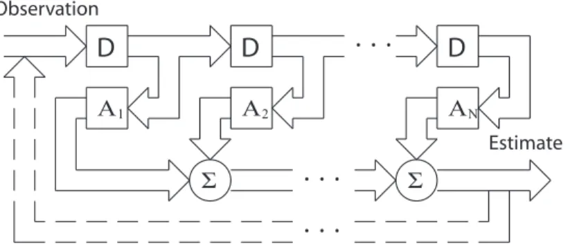
CHAPTER 3. PROBLEM DEFINITION AND METHODS 28 Estimate Observation

D

Σ Σ A₂ A₁ A_N

. . .

Figure 3.3: The generation of the horizon by the adaptive filter. The one step estimate is generated by use of a transversal filter weighting the past observations to produce an estimate for the next expected observation. When generating predictions for the horizon, the path is closed as the last estimate is treated as the current input. The prediction sequence is the collection of the estimate output each time the filter is iterated.

CΦ0,1 where

Φ0,1 : [zn, . . . , zn−N+1]T → [ˆzn+1, zn, . . . , zn−N+2]T

C : [zn, . . . , zn−N+1]T → zn; C = [I 0 · · · 0],

then it is possible to define a matrix U such that it maps the memory of past observations to the expected horizon. In this case,

U =        CΦ0,1 CΦ2 0,1 .. . CΦM 0,1        U : (zn, zn−1, . . . , zn−N+1) → (ˆzn+1, ˆzn+2, . . . , ˆzn+M). (3.8)

(43)

Using the above described method for obtaining an estimate, the horizon is gener-ated by collecting the next M estimates of the POI trajectory. Each time the process starts, the current state vector is composed of N-1 past observations together with the current observation. The first one-step prediction is generated by this state vec-tor. Then, the state vector is shifted down by one observation size and the new prediction is used as the current observation. By following this procedure the next M estimates in the prediction horizon are generated (see Figure 3.3). This collec-tion of M estimates is the expected POI trajectory given the N-1 past observacollec-tions and the current observation. In order to generate next prediction horizon at the following time step, the aforementioned procedure is applied to the new state vector where the new state vector is composed of the new actual heart position data and corresponding N − 1 past observations.

3.3 Generalized Linear Prediction

In Section 3.2, the optimal linear one step predictor, in the sense of prediction er-ror magnitude, was formulated and used recursively to generate predictions. This method approximates the heart dynamics as being a linear discrete time system and leads to sub-ideal predictions, as the POI motion has nonlinear dynamics. In the generalized prediction method that is explained in this section, the assumption of a linear system relation between consecutive time samples is abandoned. Instead, a linear estimator for each point in the horizon is independently estimated. This is done by extending (3.7) as follows:

V        zn z_n−1 .. . z_n−N+1        =        ˆ zn+1 ˆ zn+2 .. . ˆ zn+M        (3.9)

(44)

Where V is the estimation matrix that maps from the collection of observations to the expected horizon. In the same way as W was parameterized, RLS is used to determine V online and adaptively. However, since (3.9) contains the estimated values that are being solved for, it is unsuitable for implementation via RLS as is. This can be solved by assuming POI statistics to be stationary, or at least slowly varying, which makes V approximately constant. The assumption of time invariance of the heart statistics is utilized to introduce M delays so that all quantities have been observed when solving for V .

V        z_n−M z_{n−M −1} ... z_{n−N−M +1}        =        z_{n−M +1} z_{n−M +2} ... zn        (3.10)

The analogy can be made between (3.10) and an adaptive filter. The right hand side is the desired output and the observation vector on the left hand side is the input. Further, introducing the estimation matrices

Φ0,i : [zn, . . . , zn−N+1]T → [ˆzn+i, ˆzn+i+1, . . . , ˆz−N +n+i] T

for 1 ≤ i ≤ M, then V can be decomposed similar to U in (3.8) as

V =        CΦ0,1 CΦ0,2 .. . CΦ0,M        (3.11)

The generalization of this prediction method results from the fact that, unlike in (3.8), Φ0,i are parameterized independently and not, in general, equal to Φi0,1.

(45)

The removal of this constraint allows for the nonlinear dynamics throughout the prediction horizon to be better predicted by a linear estimator.

The predictor is implemented in a similar way to the previous vector RLS adap-tive filter. The adapadap-tive filter is formulated to solve the delayed estimation equation (3.10). This is equivalent to using a bank of n-step predictors, but is more computa-tionally efficient. The largest cost in the RLS algorithm involves updating the inverse covariance matrix of the inputs. The generalized predictor is an improvement on to the one-step predictor, since in generalized predictor each estimate is using the same input vector. As a result the updating only needs to be done once, providing a dra-matic reduction in computational complexity of one-step predictor when predictions are being made at many points throughout the horizon.

(46)

Chapter 4 Experimental Results

In this chapter, we evaluate the performance of the prediction methods that we pre-sented in the previous chapter. In the literature these predictors are tested with very limited and short duration of data. In this research, these algorithms are extensively studied with a wide range of different heart motion data. This is the first study that uses real varying heart rate data to perform heart motion tracking.

We start by introducing our testbed and the performance metrics we use. Next, we compare the performance of existing methods in terms of these metrics on both constant and varying heart rate data. Finally, we compare the presented results with the reported values in the literature and show that the presented generalized predictor outperforms existing methods for heart motion tracking.

(47)

CHAPTER 4. EXPERIMENTAL RESULTS 33

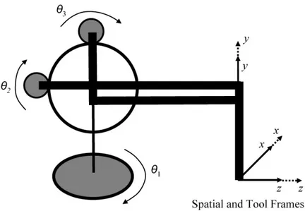
Figure 4.1: Zero Configuration of the PHANToM manipulator, also showing the axes movements and spatial and tool frames.

4.1 Experiments and Results

4.1.1 3-DOF Robotic Testbed

The proposed estimation algorithms were tested on a PHANToM Premium 1.5A haptic device, which is a 3-DOF robotic system. The nonlinearities of the system (i.e., gravitational effects, joint frictions, and Coriolis and centrifugal forces) were canceled independently from the controller. In order to maintain the accuracy of the experiments, the manipulator was brought to a selected home (zero) position, in the center of its workspace (more details can be found in [24]), before every experiment. The controller used by Bebek and Cavusoglu [4] was modified to include the new prediction algorithms. The trials used the prerecorded heart motion data described in Section 2.2. The robot was made to follow the combined motion of heartbeat and breathing. The system was run using online streaming position data in place

(48)

of real-time measurements. The controller was implemented in xPC Target and run in real time with a sampling time of 0.5 ms on a Intel Xeon 2.33 GHz Core PC. The linearized robot model was controlled using RHMPC. The RHMPC was formulated to track the horizon estimate weighted by a quadratic objective function. The encoder positions on the PHANToM were recorded and these positions were transformed into end effector positions. The reported RMS errors are calculated from the difference between the prerecorded target point and the actual end effector position calculated from joint angles.

4.1.2 Simulation and Experimental Results

The same control method and reference data were used while running simulations and experiments. During the trials, a 16th _{order correlated signal one-step estimator and}

a 10th _{order generalized estimator predicting 4 different future points in the 25 ms}

horizon were used and quadratic interpolation was accounted for the intermittent points. The experiments were carried out using two different constant heart rate data and four different varying heart rate data.

Experiments were run 10 times with the estimation algorithms and again with the actual heart motion data as future signal reference for the prediction horizon. The later case represents a ‘perfect’ estimation, providing a performance base of the robotic system’s capability. It was noted that the deviation between the trials are very small. Among these results, the maximum values for the End-effector RMS and Maximum Position Errors in millimeters in 3D and RMS Control Effort in millinewton meters are summarized in Table 4.1 for simulations and in Table 4.2 for experiments to project the worst cases. The results shown in Tables 4.1 and 4.2 are grouped with respect to type of the heart rate data collected from the animals. The position of the Sonomicrometer crystal on the heart surface, which are named as ‘Top’ position and ‘Side’ position are also stated.

(49)

SIMULATION AND EXPERIMENTAL RESULTS: The fixed heart rate data from animal 1 is 235 s long with a sampling rate of 257 Hz and from animal 2 is 472 s long with a sampling rate of 404 Hz. The sampling rate of all data sets with varying heart rate are 404 Hz. The duration of the varying heart rate data from animal 1 is 251 s for top position and 250 s for the side position. The duration for the varying heart from animal 3 is 200 s for top position and 140 s for side position.

Table 4.1: Simulation Results for End-Effector Tracking

A - RMS Position Error and MAX Position Error for the Control Algo-rithms

End-effector Tracking Results

RMS Position Error [mm] (Maximum Position Error [mm])

Heart Rate Fixed Varying

DataSet Animal 1 Animal 2 Animal 1 Animal 3 Animal 1 Animal 3

Crystal Position Top Top Top Top Side Side

RHMPC with Exact Reference Information

0.488 0.237 0.231 0.197 0.194 0.231

(1.428) (1.236) (0.777) (0.650) (1.542) (1.033) RHMPC with One-Step

Adaptive Filter Estimation

0.524 0.255 0.247 0.206 0.201 0.237

(1.953) (1.460) (1.098) (0.917) (2.163) (1.195) RHMPC with Generalized

0.481 0.235 0.229 0.195 0.191 0.230

(1.399) (1.173) (0.767) (0.861) (1.540) (1.059)

B - RMS Control Effort for the Control Algorithms

Control Effort [mNm]

RHMPC with Exact Reference

Information 18.873 14.589 16.647 11.719 13.675 14.137

RHMPC with One-Step

Adaptive Filter Estimation 26.685 21.801 37.991 18.010 30.402 20.027

RHMPC with Generalized

(50)

Table 4.2: Experiment Results for End-Effector Tracking

A - RMS Position Error and MAX Position Error for the Control Algo-rithms

RMS Position Error [mm] (Maximum Position Error [mm])

RHMPC with Exact Reference Information

0.344 0.162 0.163 0.171 0.161 0.165

(1.238) (0.912) (0.780) (0.559) (0.538) (0.906) RHMPC with One-Step

0.404 0.176 0.181 0.199 0.173 0.188

(2.236) (1.395) (1.576) (1.084) (0.960) (1.022) RHMPC with Generalized

0.351 0.174 0.168 0.178 0.164 0.167

(1.291) (1.022) (0.827) (0.615) (0.572) (0.972)

B - RMS Control Effort for the Control Algorithms

Control Effort [mNm]

RHMPC with Exact Reference

Information 54.379 28.512 25.350 21.593 24.390 27.260

RHMPC with One-Step

Adaptive Filter Estimation 55.686 33.785 46.820 24.346 52.640 29.592

RHMPC with Generalized

(51)

Tracking results for a constant heart rate data with the one-step estimator in two different scales is shown in Figure 4.2 and results for varying heart rate data with the generalized adaptive filter estimation is shown in Figure 4.3. When Figure 4.2-A and Figure 4.3-A are compared, the variations in the heart rate can be observed from the pattern of the reference signal for x-axis in Figure 4.3-A. In Figure 4.2-B and Figure 4.3-B, magnitude of the end effector position error superimposed with the reference signal for the x-axis is shown.

(52)

CHAPTER 4. EXPERIMENTAL RESULTS 38 20 40 60 80 100 120 140 160 0 2 4 6 8 10 Time [s] Position [mm] A−x−Axis Reference Ref x 1100 112 114 116 118 120 122 124 126 128 2 4 6 8 10 Time [s] Position [mm]

B−End Effector Position Error and x−Axis Reference

Ref x Err

x

Figure 4.2: Tracking results for 157-s constant heart rate heart motion data in two different scales with RHMPC with One-Step Adaptive Filter Estimation. (A) The reference signal for the x-axis. (B) Magnitude of the end effector error (below) superimposed with the reference signal for the x-axis.

We believe that, the maximum error values are affected from the noise in the data collected by Sonomicrometry sensor as it is unlikely that the POI on the heart is capable of moving 5 mm in a few milliseconds. The data has been kept as-is without applying any filtering to eliminate these jumps in the sensor measurement data as currently we do not have an independent set of sensor measurements (such as from a vision sensor) that would confirm this conjecture.

As it can be seen from the results presented in Table 4.1, in our simulations the generalized estimator out performed the exact heart signal in terms of RMS Position error. This is likely due a combination of two factors. First, the simulation model is a linearized, reduced order model of the actual hardware. Second, the estimator has a robustness characteristic that makes its output less noisy than the actual

(53)

CHAPTER 4. EXPERIMENTAL RESULTS 39 20 40 60 80 100 120 140 160 180 200 0 1 2 3 4 5 6 7 8 Time [s] Position [mm] A−x−Axis Reference Ref x 70 72 74 76 78 80 82 84 86 88 0 1 2 3 4 5 6 7 8 Time [s] Position [mm]

B−End Effector Position Error and x−Axis Reference

Ref x Err

x

Figure 4.3: Tracking results for 200-s varying heart rate heart motion data in two different scales with RHMPC with Generalized Adaptive Filter Estimation. (A) The reference signal for the x-axis. (B) Magnitude of the end effector error (below) superimposed with the reference signal for the x-axis.

heart data. The combination of these two factors yields better results in the linear case. However, when the experiment is performed on the hardware, the effects of the nonlinearities are seen when the performance of the estimator-driven controller decreases. It should be noted that although the simulation provides valuable insight to the effectiveness of the controller, it is the experimental trials that are the best indicator of performance.

When the tracking results of the adaptive predictors are compared with each other, the generalized predictor outperforms the one-step predictor both in simula-tions and experiments. These results show that the nonlinear dynamics of the POI throughout the prediction horizon are better predicted by a generalized estimator.

(54)

From the results presented in Table 4.2, it can be observed that, in the ex-periments the controller with exact heart signal reference performs better than the one-step estimator and the generalized estimator in term RMS end effector error for both constant heart rate data and varying heart rate data. Maximum error and the control effort results for the exact heart signal are also smaller than the tracking re-sults of one-step and generalized estimators, because the controller with exact heart signal reference represents the perfect estimation for heart motion tracking.

4.1.3 Discussion of the Results

At this point, it would be informative to compare the presented tracking results with the reported values in the literature.

Ginhoux et al. [7] used motion canceling through prediction of future heart motion using high-speed visual servoing with a model predictive controller. Their results indicated a tracking error variance on the order of 6-7 pixels (approximately 1.5-1.75 mm calculated from the 40 pixel/cm resolution reported in [7]) in each direction of a 3-DOF tracking task. Although it yielded better results than earlier studies using vision systems, the error was still very large to perform heart surgery.

Bebek and Cavusoglu used the past heartbeat cycle motion data, synchronized with the ECG data, in their estimation algorithms. They achieved 0.682 mm RMS end-effector position error on a 3-DOF robotic test-bed system [4].

Yuen et al. used an Extended Kalman Filter (EKF) algorithm with a quasiperi-odic motion model to predict the path of mitral valve motion in order to compensate the time delay occurred from the 3-dimensional ultrasound (3DUS) measurements. They achieved 1.15 ± 0.004 mm RMS tracking error for a 1-DOF motion compensa-tion instrument (MCI) in an in vitro 3DUS-guided servoing test. They stated that employing the EKF based predictor in time-delay compensation restores the tracking

Heart motion prediction based on adaptive estimation aşgorithms fo robotic-assisted beating heart surgery

HEART MOTION PREDICTION BASED ON ADAPTIVE

ESTIMATION ALGORITHMS FOR ROBOTIC-ASSISTED

BEATING HEART SURGERY

a thesis

submitted to the department of electrical and

electronics engineering

and the graduate school of engineering and science

of bilkent university

in partial fulfillment of the requirements

for the degree of

master of science

By

Eser Erdem Tuna

September, 2011

ABSTRACT

HEART MOTION PREDICTION BASED ON ADAPTIVE

ESTIMATION ALGORITHMS FOR ROBOTIC-ASSISTED

BEATING HEART SURGERY

¨

OZET

ROBOT˙IK-DESTEKL˙I KALP AMEL˙IYATLARI ˙IC

¸ ˙IN

UYAB˙ILEN TAHM˙IN ALGOR˙ITMALARINA DAYALI

KALP HAREKET˙I TAHM˙IN˙I

Acknowledgement

Dedeme ve anneanneme

Contents

List of Figures

List of Tables

Chapter 1

Introduction

1.1

Coronary Artery Bypass Graft Surgery

1.2

Robotic-Assisted Beating Heart Surgery

1.3

Motion Estimation Algorithms for Model

Based Active Relative Motion Canceling

Al-gorithms

1.4

A Probabilistic Robotics Approach for

Sens-ing

1.5

Contributions

1.6

Thesis Outline

Chapter 2

Background

2.1

Related Works in Literature

2.2

Analysis of Heart Data

2.2.1

Experimental Setup for Measurement of Heart Motion

2.2.2

Analysis of Varying Heart Rate Motion Data

Chapter 3

Problem Definition and Methods

3.1

Problem Formulation

3.2

One Step Motion Estimation Algorithm

3.2.1

Model of Heart Motion

3.2.2

Adaptive Filter

D

3.2.3

Parametrization

3.2.4

Recursive Least Squares

3.2.5

Prediction

D

D

D

. . .

. . .

. . .