SIAM J. SCI. COMPUT. c 2018 Society for Industrial and Applied Mathematics Vol. 40, No. 1, pp. C25–C46
1.5D PARALLEL SPARSE MATRIX-VECTOR MULTIPLY∗
ENVER KAYAASLAN†, CEVDET AYKANAT‡, AND BORA UC¸ AR§
Abstract. There are three common parallel sparse matrix-vector multiply algorithms: 1D row-parallel, 1D column-parallel, and 2D row-column-parallel. The 1D parallel algorithms offer the advantage of having only one communication phase. On the other hand, the 2D parallel algorithm is more scalable, but it suffers from two communication phases. Here, we introduce a novel concept of heterogeneous messages where a heterogeneous message may contain both input-vector entries and partially computed output-vector entries. This concept not only leads to a decreased number of messages but also enables fusing the input- and output-communication phases into a single phase. These findings are exploited to propose a 1.5D parallel sparse matrix-vector multiply algorithm which is called local row-column-parallel. This proposed algorithm requires a constrained fine-grain partitioning in which each fine-grain task is assigned to the processor that contains either its input-vector entry, its output-input-vector entry, or both. We propose two methods to carry out the constrained fine-grain partitioning. We conduct our experiments on a large set of test matrices to evaluate the partitioning qualities and partitioning times of these proposed 1.5D methods.
Key words. sparse matrix partitioning, parallel sparse matrix-vector multiplication, directed hypergraph model, bipartite vertex cover, combinatorial scientific computing
AMS subject classifications. 05C50, 05C65, 05C70, 65F10, 65F50, 65Y05
DOI. 10.1137/16M1105591
1. Introduction. Sparse matrix-vector multiply (SpMV) of the form y← Ax is a fundamental operation in many iterative solvers for linear systems, eigensystems, and least squares problems. This renders the parallelization of SpMV operation an important problem. In the literature, there are three SpMV algorithms: row-parallel, column-parallel, and row-column-parallel. Row-parallel and column-parallel (called 1D) algorithms have a single communication phase, in which either the x-vector or partial results on the y-vector entries are communicated. Row-column-parallel (2D) algorithms have two communication phases. First, the x-vector entries are commu-nicated, and then the partial results on the y-vector entries are communicated. We propose another parallel SpMV algorithm in which both the x-vector and the partial results on the y-vector entries are communicated as in the 2D algorithms, yet the communication is handled in a single phase as in the 1D algorithms. That is why the new parallel SpMV algorithm is dubbed 1.5D.
Partitioning methods based on graphs and hypergraphs are widely established to achieve 1D and 2D parallel algorithms. For 1D parallel SpMV, row-wise or column-wise partitioning methods are available. The scalability of 1D parallelism is limited especially when a row or a column has too many nonzeros in the row- and column-parallel algorithms, respectively. In such cases, the communication volume is high, and the load balance is hard to achieve, severely reducing the solution space. The associated partitioning methods are usually the fastest alternatives. For 2D parallel ∗Submitted to the journal’s Software and High-Performance Computing section December 2, 2016; accepted for publication (in revised form) July 31, 2017; published electronically February 1, 2018. A preliminary version appeared in IPDPSW [12].
http://www.siam.org/journals/sisc/40-1/M110559.html
†NTENT, Inc., 1808 Aston Ave., Carlsbad, CA 92008 ([email protected]).
‡Bilkent University, Department of Computer Engineering, Ankara TR-06800, Turkey ([email protected]).
§CNRS and LIP (UMR5668 CNRS-ENS Lyon-INRIA-UCBL), 46, all´ee d’Italie, ENS Lyon, Lyon 69364, France ([email protected]).
C26 E. KAYAASLAN, C. AYKANAT, AND B. UC¸ AR
SpMV, there are different partitioning methods. Among them, those that partition matrix entries individually, based on the fine-grain model [4], have the highest flexi-bility. That is why they usually obtain the lowest communication volume and achieve near perfect balance among nonzeros per processor [7]. However, the fine-grain par-titioning approach usually results in higher number of messages; not surprisingly, a higher number of messages hampers the parallel SpMV performance [11].
The parallel SpMV operation is composed of fine-grain tasks of multiply-and-add operations of the form yi ← yi+ aijxj. Here, each fine-grain task is identified
with a unique nonzero and assumed to be performed by the processor that holds the associated nonzero by the owner-computes rule. The proposed 1.5D parallel SpMV imposes a special condition on the operands of the fine-grain task yi ← yi+ aijxj:
The processor that holds aij should also hold xj or should be responsible for yi
(or both). The standard row-wise and column-wise partitioning algorithms for 1D parallel algorithms satisfy the condition, but they are too restrictive. The standard fine-grain partitioning approach does not necessarily satisfy the condition. Here, we propose two methods for partitioning for 1.5D parallel SpMV. With the proposed partitioning methods, the overall 1.5D parallel SpMV algorithm inherits the important characteristics of 1D and 2D parallel SpMV and the associated partitioning methods. In particular, it has
• a single communication phase as in 1D parallel SpMV;
• the partitioning flexibility close to that of 2D fine-grain partitioning; • a much-reduced number of messages compared to the 2D fine-grain
partition-ing;
• a partitioning time close to that of 1D partitioning.
We propose two methods (section 4) to obtain a 1.5D local fine-grain partition each with a different setting and approach where some preliminary studies on these methods are given in our recent work [12]. The first method is developed by proposing a directed hypergraph model. Since current partitioning tools cannot meet 1.5D partitioning requirements, we adopt and adapt an approach similar to that of a recent work by Pelt and Bisseling. [15]. The second method has two parts. The first part applies a conventional 1D partitioning method but decodes this only as a partition of the vectors x and y. The second part decides nonzero/task distribution under the fixed partition of the input and output vectors.
The remainder of this paper is as follows. In section 2, we give a background on parallel SpMV. Section 3 presents the proposed 1.5D local row-column-parallel algorithm and 1.5D local fine-grain partitioning. The two methods proposed to obtain a local fine-grain partition are presented and discussed in section 4. Section 5 gives a brief review of recent related work. We display our experimental results in section 6 and conclude the paper in section 7.
2. Background on parallel sparse matrix-vector multiply.
2.1. The anatomy of parallel sparse matrix-vector multiply. Recall that y← Ax can be cast as a collection of fine-grain tasks of multiply-and-add operations
(1) yi← yi+ aij× xj.
These tasks can share input and output-vector entries. When a task aij and the
input-vector entry xjare assigned to different processors, say, P`and Pr, respectively,
Pr sends xj to P`, which is responsible to carry out the task aij. An input-vector
entry xj is not communicated multiple times between processor pairs. When a task
1.5D PARALLEL SPARSE MATRIX-VECTOR MULTIPLY C27 P1 P2 P3 P1 P2 P3 x1 x1 x2 x2 x3 x3 y1 y1 y2 y2 a12 a12 a13 a13 a21 a21 a22 a22 3 2 2 1 1 P1 P1 P2 P2 P3 P1 P2 P2 P3 P3 P2 P1 3 2 2 1 1 P2 P2 P3 P1 P1 P1 P3 P2 P2 P2 P3 P1 P2
Fig. 1. A task-and-data distribution Π(y ← Ax) of matrix-vector multiply with a 2 × 3 sparse matrix A.
aij and the output-vector entry yi are assigned to different processors, say, Pr and
Pk, respectively, Pr performs ˆyi← ˆyi+ aij× xj as well as all other multiply-and-add
operations that contribute to the partial result ˆyiand then sends ˆyito Pk. The partial
results received by Pk from different processors are then summed to compute yi.
2.2. Task-and-data distributions. Let A be an m×n sparse matrix and aij
represent both a nonzero of A and the associated fine-grain task of multiply-and-add operation (1). Let x and y be the input- and output-vectors of size n and m, respectively, and K be the number of processors. We define a K-way task-and-data distribution Π(y← Ax) of the associated SpMV as a 3-tuple Π(y ← Ax) = (Π(A), Π(x), Π(y)), where Π(A) = {A(1), . . . , A(K)
}, Π(x) = {x(1), . . . , x(K)
}, and Π(y) ={y(1), . . . , y(K)
}. We can also represent Π(A) as a nonzero-disjoint summation
(2) A= A(1)+ A(2)+
· · · + A(K).
In Π(x) and Π(y), each x(k) and y(k) is a disjoint subvector of x and y, respectively.
Figure 1 illustrates a sample 3-way task-and-data distribution of matrix-vector mul-tiply on a 2×3 sparse matrix.
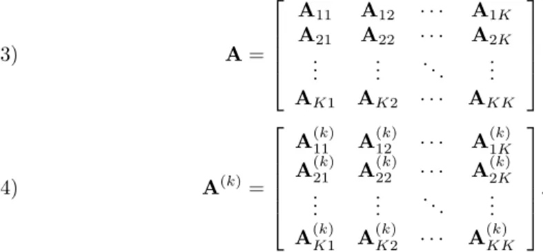
For given input- and output-vector distributions Π(x) and Π(y), the columns and rows of A and those of A(k) can be permuted, conformably with Π(x) and Π(y), to
form K×K block structures:
A= A11 A12 · · · A1K A21 A22 · · · A2K .. . ... . .. ... AK1 AK2 · · · AKK (3) A(k)= A(k)11 A(k)12 · · · A(k)1K A(k)21 A(k)22 · · · A(k)2K .. . ... . .. ... A(k)K1 A(k)K2 · · · A(k)KK . (4)
Note that the row and column orderings (4) of the individual A(k) matrices are in
compliance with the row and column orderings (3) of A. Hence, each block Ak` of
the block structure (3) of A can be written as a nonzero-disjoint summation
(5) Ak`= A(1)k` + A
(2)
k` +· · · + A (K)
k` .
Let Π(y ← Ax) be any K-way task-and-data distribution. According to this distribution, each processor Pk holds the submatrix A(k), holds the input-subvector
C28 E. KAYAASLAN, C. AYKANAT, AND B. UC¸ AR
x(k), and is responsible for storing/computing the output subvector y(k). The
fine-grain tasks (1) associated with the nonzeros of A(k) are to be carried out by P
k.
An input-vector entry xj ∈ x(k) is sent from Pk to P`, which is called an input
communication, if there is a task aij ∈ A(`) associated with a nonzero at column j.
On the other hand, Pk receives a partial result ˆyion an output-vector entry yi∈ y(k)
from P`, which is referred to as an output communication, if there is a task aij ∈ A(`)
associated with a nonzero at row i. Therefore, the fine-grain tasks associated with the nonzeros of the column stripe A∗k = [AT1k, . . . , ATKk]T are the only ones that require
an input-vector entry of x(k), and the fine-grain tasks associated with the nonzeros
of the row stripe Ak∗ = [Ak1, . . . , AkK] are the only ones that contribute to the
computation of an output-vector entry of y(k).
2.3. 1D parallel sparse matrix-vector multiply. There are two main alter-natives for 1D parallel SpMV: row-parallel and column-parallel.
In the row-parallel SpMV, the basic computational units are the rows. For an output-vector entry yi assigned to processor Pk, the fine-grain tasks associated with
the nonzeros of Ai∗ ={aij ∈ A : 1 ≤ j ≤ n} are combined into a composite task of
inner product yi ← Ai∗x, which is to be carried out by Pk. Therefore, for the
row-parallel algorithm, a task-and-data distribution Π(y←Ax) of matrix-vector multiply on A should satisfy the following condition:
(6) aij ∈ A(k) whenever yi∈ y(k).
Then Π(A) coincides with the output-vector distribution Π(y)—each submatrix is a row stripe of the block structure (3) of A. In the row-parallel parallel SpMV, all messages are communicated in an input-communication phase called expand, where each message contains only input-vector entries.
In the column-parallel SpMV, the basic computational units are the columns. For an input-vector entry xjassigned to processor Pk, the fine-grain tasks associated with
the nonzeros of A∗j ={aij ∈ A : 1 ≤ i ≤ m} are combined into a composite task of
“daxpy” operation ˆyk ← ˆyk+ A∗jxj, which is to be carried out by Pk, where ˆyk is
the partially computed output-vector of Pk. As a result, a task-and-data distribution
Π(y← Ax) of matrix-vector multiply on A for the column-parallel algorithm should satisfy the following condition:
(7) aij ∈ A(k) whenever xj∈ x(k).
Here, Π(A) coincides with the input-vector distribution Π(x)—each submatrix A(k)
is a column stripe of the block structure (3) of A. In the column-parallel SpMV, all messages are communicated in an output-communication phase called fold, where each message contains only partially computed output-vector entries.
The column-net and row-net hypergraph models [3] can be used to obtain the required task-and-data partitioning for, respectively, the row-parallel and column-parallel SpMV.
2.4. 2D parallel sparse matrix-vector multiply. In the 2D parallel SpMV, also referred to as the row-column-parallel, the basic computational units are nonze-ros [4, 7]. The row-column-parallel algorithm requires fine-grain partitioning, which imposes no restriction on distributing tasks and data. The row-column-parallel algo-rithm contains two communication and two computational phases in an interleaved manner as shown in Algorithm 1. The algorithm starts with the expand phase, where the required input-subvector entries are communicated. The second step computes
1.5D PARALLEL SPARSE MATRIX-VECTOR MULTIPLY C29 Algorithm 1. The row-column-parallel sparse matrix-vector multiply.
For each processor Pk:
1. (expand) for each nonzero column stripe A(`)∗k, where `6= k;
(a) form vector ˆx(k)` , which contains only those entries of x(k)corresponding
to nonzero columns in A(`)∗k, and (b) send vector ˆx(k)` to P`.
2. for each nonzero row stripe A(k)`∗, where `6= k; compute (a) y(`)k ← A(k)`k x(k) and (b) y(`)k ← yk(`)+P r6=kA (k) `rxˆ (r) k .
3. (fold) for each nonzero row stripe A(k)`∗ , where `6= k;
(a) form vector ˆy(`)k , which contains only those entries of y(`)k corresponding to nonzero rows in A(k)`∗, and
(b) send vector ˆy(`)k to P`. 4. compute output-subvector (a) y(k) ← A(k)kkx(k), (b) y(k) ← y(k)+ A(k) k`xˆ (`) k , and (c) y(k) ← y(k)+P `6=kyˆ (k) ` .
only those partial results that are to be communicated in the following fold phase. In the final step, each processor computes its own output-subvector. If we have a row-wise partitioning, steps 2, 3, and 4c are not needed, and hence the algorithm reduces to the row-parallel algorithm. Similarly, the algorithm without steps 1, 2b, and 4b can be used when we have a column-wise partitioning. The row-column-net hypergraph model [4, 7] can be used to obtain the required task-and-data partitioning for row-column-parallel SpMV.
3. 1.5D parallel sparse matrix-vector multiply. In this section, we propose the local row-column-parallel SpMV algorithm that exhibits 1.5D parallelism. The proposed algorithm simplifies the row-column-parallel algorithm by combining the two communication phases into a single expand-fold phase while attaining a flexibility on nonzero/task distribution close to the flexibility attained by the row-column-parallel algorithm.
In the well-known parallel SpMV, the messages are homogeneous in the sense that they pertain to either x- or y-vector entries. In the proposed row-column-parallel SpMV algorithm, the number of messages is reduced with respect to the row-column-parallel algorithm by making the messages heterogeneous (pertaining to both x- and y-vector entries) and by communicating them in a single expand-fold phase. If a processor P`sends a message to processor Pk in both the expand and the fold phases,
then the number of messages required from P`to Pkreduces from two to one. However,
if a message from P`to Pk is sent only in the expand phase or only in the fold phase,
then there is no reduction in the number of such messages.
3.1. A task categorization. We introduce a 2-way categorization of input- and output-vector entries and a four-way categorization of fine-grain tasks (1) according
C30 E. KAYAASLAN, C. AYKANAT, AND B. UC¸ AR
to a task-and-data distribution Π(y← Ax) of matrix-vector multiply on A. For a task aij, the input-vector entry xj is said to be local if both aij and xj are assigned
to the same processor; the output-vector entry yiis said to be local if both aij and yi
are assigned to the same processor. With this definition, the tasks can be classified into four groups. The task
yi← yi+ aij× xj on Pk is input-output-local if xj∈ x(k)and yi∈ y(k), input-local if xj∈ x(k)and yi6∈ y(k), output-local if xj6∈ x(k)and yi∈ y(k), nonlocal if xj6∈ x(k)and yi6∈ y(k).
Recall that an input-vector entry xj ∈ x(`) is sent from P`to Pk if there exists a task
aij ∈ A(k)at column j, which implies that the task aij of Pk is either output-local or
nonlocal since xj 6∈ x(k). Similarly, for an output-vector entry yi ∈ y(`), P` receives
a partial result ˆyi from Pk if a task aij ∈ A(k), which implies that the task aij of Pk
is either input-local or nonlocal since yi6∈ y(k). We can also infer from this that the
input-output-local tasks neither depend on the input-communication phase nor incur a dependency on the output-communication phase. However, the nonlocal tasks are linked with both communication phases.
In the row-parallel algorithm, each of the fine-grain tasks is either input-output-local or output-input-output-local due to the row-wise partitioning condition (6). For this reason, no partial result is computed for other processors, and thus no output communication is incurred. In the column-parallel algorithm, each of the fine-grain tasks is either input-output-local or input-local due to the column-wise partitioning condition (7). In the row-column-parallel algorithm, the input and output communications have to be carried out in separate phases. The reason is that the partial results on the output-vector entries to be sent are partially derived by performing nonlocal tasks that rely on the input-vector entries received.
3.2. Local fine-grain partitioning. In order to remove the dependency be-tween the two communication phases in the row-column-parallel algorithm, we pro-pose the local fine-grain partitioning where “locality” refers to the fact that each fine-grain task is input-local, output-local, or input-output-local. In other words, there is no nonlocal fine-grain task.
A task-and-data distribution Π(y← Ax) of matrix-vector multiply on A is said to be a local fine-grain partition if the following condition is satisfied:
(8) aij ∈ A(k)+ A(`) whenever yi∈ y(k)and xj∈ x(`).
Notice that this condition is equivalent to
(9) if aij∈ A(k) then either xj∈ y(k), yi∈ x(k), or both.
Due to (4) and (9), each submatrix A(k) becomes of the following form:
(10) A(k)= 0 . . . A(k)1k . . . 0 .. . . .. ... . .. ... A(k)k1 · · · A(k)kk · · · A(k)kK .. . . .. ... . .. ... 0 . . . A(k)Kk . . . 0 .
1.5D PARALLEL SPARSE MATRIX-VECTOR MULTIPLY C31 P1 P2 P3 P1 P2 P3 x1 x1 x2 x2 x3 x3 y1 y1 y2 y2 a12 a12 a13 a13 a21 a21 a22 a22 3 2 2 1 1 P1 P1 P2 P2 P3 P1 P2 P2 P3 P3 P2 P1 3 2 2 1 1 P2 P2 P3 P1 P1 P1 P3 P2 P2 P2 P3 P1 P2
Fig. 2. A sample local fine-grain partition. Here, a12 is an output-local task, a13is an input-output-local task, a21is an output-local task, and a22is an input-local task.
In this form, the tasks associated with the nonzeros of diagonal block A(k)kk, the off-diagonal blocks of the row stripe A(k)k∗, and the off-diagonal blocks of the column-stripe A(k)∗k are input-output-local, output-local, and input-local, respectively. Furthermore, due to (5) and (8), each off-diagonal block Ak`of the block structure (3) induced by
the vector distribution (Π(x),Π(y)) becomes
(11) Ak`= A(k)k` + A
(`)
k`,
and for each diagonal block we have Akk= A(k)kk.
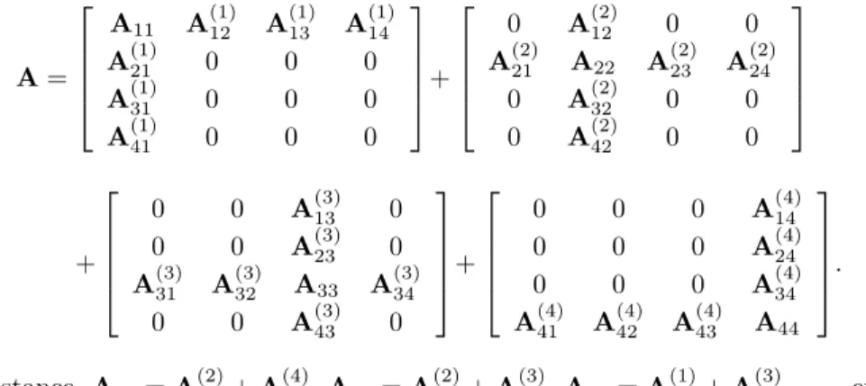
In order to clarify equations (8)–(11), we provide the following 4-way local fine-grain partition on A as permuted into a 4×4 block structure:
A= A11 A(1)12 A (1) 13 A (1) 14 A(1)21 0 0 0 A(1)31 0 0 0 A(1)41 0 0 0 + 0 A(2)12 0 0 A(2)21 A22 A(2)23 A (2) 24 0 A(2)32 0 0 0 A(2)42 0 0 + 0 0 A(3)13 0 0 0 A(3)23 0 A(3)31 A(3)32 A33 A(3)34 0 0 A(3)43 0 + 0 0 0 A(4)14 0 0 0 A(4)24 0 0 0 A(4)34 A(4)41 A(4)42 A(4)43 A44 . For instance, A42= A(2)42 + A (4) 42, A23= A(2)23 + A (3) 23, A31= A(1)31 + A (3) 31, . . . , etc.
Figure 2 displays a sample 3-way local fine-grain partition on the same sparse matrix used in Figure 1. In this figure, a13∈ A(1), where y1∈ y(2) and x3∈ x(1) and
thus a13 is an input-local task of P1. Also, a21∈ A(3) where y2∈ y(3) and x1∈ x(1)
and thus a21 is an output-local task of P3.
3.3. Local row-column-parallel sparse matrix-vector multiply. As there are no nonlocal tasks, the output-local tasks depend on input communication, and the output communication depends on the input-local tasks. Therefore, the task groups and communication phases can be arranged as (i) input-local tasks; (ii) output-communication, input-communication; and (iii) output-local tasks and input-output-local tasks. The input and output communication phases can be combined into the expand-fold phase, and the output-local and input-output-local task groups can be combined into a single computation phase to simplify the overall execution.
The local row-column-parallel algorithm is composed of three steps as shown in Algorithm 2. In the first step, processors concurrently perform their input-local tasks which contribute to partially computed output-vector entries for other processors. In
C32 E. KAYAASLAN, C. AYKANAT, AND B. UC¸ AR
Algorithm 2. The local row-column-parallel sparse matrix-vector multiply. For each processor Pk:
1. for each nonzero block A(k)`k , where `6= k;
compute y(`)k ← A(k)`k x(k). I input-local tasks of Pk
2. (expand-fold) for each nonzero block A`k = A(k)`k + A (`)
`k, where `6= k;
(a) form vector ˆx(k)` , which contains only those entries of x(k)corresponding
to nonzero columns in A(`)`k;
(b) form vector ˆyk(`), which contains only those entries of y(`)k corresponding to nonzero rows in A(k)`k ; and
(c) send vector [ˆx(k)` , ˆy(`)k ] to processor P`.
3. compute output-subvector (a) y(k) ← A(k)kkx(k), I input-output-local tasks of Pk (b) y(k)← y(k)+ A(k) k`xˆ (`)
k and I output-local tasks of Pk
(c) y(k)
← y(k)+P
`6=kyˆ
(k)
` . I input-local tasks of other processors
the expand-fold phase, for each nonzero off-diagonal block A`k = A(k)`k + A (`)
`k, Pk
prepares a message [ˆx(k)` , ˆy(`)k ] for P`. Here, ˆx(k)` contains the input-vector entries of
x(k)that are required by the output-local tasks of P`, whereas ˆy(`)k contains the partial
results on the output-vector entries of y(`), where the partial results are derived by
performing the input-local tasks of Pk. In the last step, each processor Pk computes
output-subvector y(k) by summing the partial results computed locally by its own
input-output-local tasks (step 3a) and output-local tasks (step 3b) as well as the partial results received from other processors due to their input-local tasks (step 3c). For a message [ˆx(k)` , ˆy(`)k ] from processor Pk to P`, the input-vector entries of ˆx(k)`
correspond to the nonzero columns of A(`)`k, whereas the partially computed output-vector entries of ˆy(`)k correspond to the nonzero rows of A(k)`k . That is, ˆx(k)` = [xj :
aij ∈ A(`)`k] and ˆy(`)k = [ˆyi : aij ∈ A(k)`k ]. This message is heterogeneous if A(k)`k and
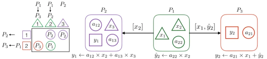
A(`)`k are both nonzero and homogeneous otherwise. We also note that the number of messages is equal to the number of nonzero off-diagonal blocks of the block structure (3) of A induced by the vector distribution (Π(x), Π(y)). Figure 3 illustrates the steps of Algorithm 2 on the sample local fine-grain partition given in Figure 2. As seen in the figure, there are only two messages to be communicated. One message is homogeneous, which is from P1 to P2 and contains only an input-vector entry x2,
whereas the other message is heterogeneous, which is from P1to P3 and contains an
input-vector entry x1and a partially computed output-vector entry ˆy2.
4. Two proposed methods for local row-column-parallel partitioning. We propose two methods to find a local row-column-parallel partition that is re-quired for 1.5D local row-column-parallel SpMV. One method finds vector and nonzero distributions simultaneously, whereas the other one has two parts in which vector and nonzero distributions are found separately.
4.1. A directed hypergraph model for simultaneous vector and nonzero distribution. In this method, we adopt the elementary hypergraph model for the
1.5D PARALLEL SPARSE MATRIX-VECTOR MULTIPLY C33 aij P` Pk xj yi xj ˆyi ˆ yi ˆyi+ aij⇥ xj yi yi+ ˆyi P` Pk P` Pk aij aij xj xj yi yi ˆ yi xj ˆ yi ˆyi+ aij⇥ xj yi yi+ ˆyi yi yi+ aij⇥ xj ˆ y2 a22⇥ x2 y1 a12⇥ x2+ a13⇥ x3 y2 a21⇥ x1+ ˆy2 P1 P2 P3 x1 x2 x3 y1 y2 a12 a13 a22 a21 [x2] [x1, ˆy2] Pr 3 2 2 1 1 P1 P1 P2 P2 P3 P1 P2 P2 P3 P3 P2 P1
Fig. 3. An illustration of Algorithm 2 for the local fine-grain partition in Figure 2.
fine-grain partitioning [16] and introduce an additional locality constraint on par-titioning in order to obtain a local fine-grain partition. In this hypergraph model H2D = (V, N ), there is an input-data vertex for each input-vector entry, an
output-data vertex for each output-vector entry, and a task vertex for each fine-grain task (or per matrix nonzero) for a given matrix A. That is,
V = {vx(j) : xj ∈ x} ∪ {vy(i) : yi ∈ y} ∪ {vz(ij) : aij ∈ A}.
The input- and output-data vertices have zero weights, whereas the task vertices have unit weights. In H2D, there is an input-data net for each input-vector entry and an
output-data net for each output-vector entry. An input-data net nx(j), corresponding
to the input-vector entry xj, connects all task vertices associated with the nonzeros at
column j as well as the input-data vertex vx(j). Similarly, an output-data net ny(i),
corresponding to the output-vector entry yi, connects all task vertices associated with
the nonzeros at row i as well as the output-data vertex vy(i). That is,
N = {nx(j) : xj∈ x} ∪ {ny(i) : yi∈ y},
nx(j) ={vx(j)} ∪ {vz(ij) : aij ∈ A, 1 ≤ i ≤ m}, and
ny(i) ={vy(i)} ∪ {vz(ij) : aij∈ A, 1 ≤ j ≤ n}.
Note that each input-data net connects a separate input-data vertex, whereas each output-data net connects a separate output-data vertex. We associate nets with their respective data vertices.
We enhance the elementary row-column-net hypergraph model by imposing di-rections on the nets; this is required for modeling the dependencies and their nature. Each input-data net nx(j) is directed from the input-data vertex vx(j) to the task
vertices connected by nx(j), and each output-data net ny(i) is directed from the task
vertices connected by ny(i) to the output-data vertex vy(i). Each task vertex vz(ij)
is connected by a single input-data-net nx(j) and a single output-data-net ny(i).
In order to impose the locality in the partitioning, we introduce the following constraint for vertex partitioning on the directed hypergraph modelH2D: Each task
vertex vz(ij) should be assigned to the part that contains either input-data vertex
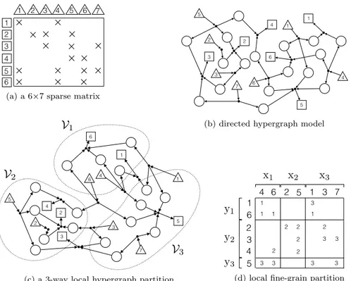
vx(j), output-data vertex vy(i), or both. Figure 4(a) displays a sample 6×7 sparse
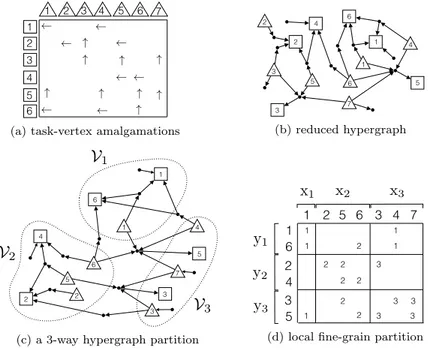
matrix. Figure 4(b) illustrates the associated directed hypergraph model. Figure 4(c) shows a 3-way vertex partition of this directed hypergraph model satisfying the lo-cality constraint, and Figure 4d shows the local fine-grain partition decoded by this partition.
Instead of developing a partitioner for this particular directed hypergraph model, we propose a task-vertex amalgamation procedure which will help in meeting the described locality constraint by using a standard hypergraph partitioning tool. For
C34 E. KAYAASLAN, C. AYKANAT, AND B. UC¸ AR 2 2 5 3 6 1 7 4
x
1x
2x
3y
1y
2y
3 1 2 3 2 5 3 4 5 6 1 6 4 1 7 3 4 1 6 5 1 1 2 2 2 2 2 3 3 3 3 2 3 3 1 3 5 3 1 2 4 5 6 7 1 2 3 4 6V
1V
2V
3 3 5 7 2 1 4 6 4 2 3 1 6 5(a) a 6×7 sparse matrix
2 2 5 3 6 1 7 4 3 5 7 4 2 2 3 1 1 6 5 6 4
x
1x
2x
3y
1y
2y
3 1 2 3 2 5 3 4 5 6 1 6 4 1 7 3 4 1 6 5 1 1 2 2 2 2 2 3 3 3 3 2 3 3 1 3P
1P
2P
3 5 3 1 2 4 5 6 7 1 2 3 4 6(b) directed hypergraph model
2 2 5 3 6 1 7 4 3 5 7 4 2 2 3 1 1 6 5 6 4
x
1x
2x
3y
1y
2y
3 1 2 3 2 5 3 4 5 6 1 6 4 1 7 3 4 1 6 5 1 1 2 2 2 2 2 3 3 3 3 2 3 3 1 3 5 3 1 2 4 5 6 7 1 2 3 4 6V
1V
2V
3 (c) a 3-way local hypergraph partition2 2 5 3 6 1 7 4 3 5 7 4 2 2 3 1 1 6 5 6 4
x
1x
2x
3y
1y
2y
3 1 2 3 2 5 3 4 5 6 1 6 1 4 7 2 3 2 5 3 4 5 6 1 6 4 1 7 3 4 1 6 5 1 1 2 2 2 2 2 3 3 3 3 2 3 3 1 3P
1P
2P
3(d) local fine-grain partition
Fig. 4. An illustration of attaining a local fine-grain partition through vertex partitioning of the directed hypergraph model that satisfies locality constraints. The input- and output-data vertices are drawn with triangles and rectangles, respectively.
this, we adopt and adapt a simple yet effective approach of Pelt and Bisseling [15]. In our adaptation, we amalgamate each task vertex vz(ij) into either input-data vertex
vx(j) or output-data vertex vy(i) according to the number of task vertices connected
by nx(j) and ny(i), respectively. That is, vz(ij) is amalgamated into vx(j) if column j
has a smaller number of nonzeros than row i; otherwise, it is amalgamated into vy(i),
where the ties are broken arbitrarily. The result is a reduced hypergraph that contains only the input- and output-data vertices amalgamated with the task vertices where the weight of a data vertex is equal to the number of task vertices amalgamated into that data vertex. As a result, the locality constraint on vertex partitioning of the initial directed hypergraph naturally holds on any vertex partitioning on the reduced hypergraph. It so happens that after this process, the net directions become irrelevant for partitioning, and hence one can use the standard hypergraph partitioning tools.
Figure 5 illustrates how to obtain a local fine-grain partition through the described task-vertex amalgamation procedure. In Figure 5(a), the up and left arrows imply that a task vertex vz(ij) is amalgamated into input-data vertex vx(j) and
output-data vertex vy(i), respectively. The reduced hypergraph obtained by these
task-vertex amalgamations is shown in Figure 5(b). Figure 5(c) and 5(d) shows a 3-way vertex partition of this reduced hypergraph and the obtained local fine-grain partition, respectively. As seen in these figures, task a35is assigned to processor P2since vz(3, 5)
is amalgamated into vx(5) and since vx(5) is assigned to V2.
We emphasize here that the reduced hypergraph constructed as above is equiv-alent to the hypergraph model of Pelt and Bisseling [15]. In that original work, the use of this model was only for 2-way partitioning (of the fine-grain model), which is
1.5D PARALLEL SPARSE MATRIX-VECTOR MULTIPLY C35 1 6 1 6 3 4 2 5 2 3 4 7 5 5 6 2 5 6 4 2 3 7 1
x
1 x2 x3y
1y
2y
3 1 4 3 1 6 5 1 2 2 2 2 3 2 1 2 3 3 3 1 1 " " " " " " " " " 2 3 2 4 6 1 5 3 2 3 4 1 7V
1V
2V
3 3 5 7 2 1 4 6 4 2 3 1 6 5(a) task-vertex amalgamations
1 6 1 6 3 4 2 5 2 3 4 7 5 5 6 2 5 6 4 2 3 7 1 3 5 7 4 2 2 3 1 1 6 5 6 4
x
1 x2 x3y
1y
2y
3 1 4 3 1 6 5 1 2 2 2 2 3 2 1 2 3 3 3 1 1P
1P
2P
3 " " " " " " " " " 2 3 2 4 6 1 5 3 2 3 4 1 7 (b) reduced hypergraph 1 6 1 6 3 4 2 5 2 3 4 7 5 5 6 2 5 6 4 2 3 7 1 3 5 7 4 2 2 3 1 1 6 5 6 4x
1 x2 x3y
1y
2y
3 1 4 3 1 6 5 1 2 2 2 2 3 2 1 2 3 3 3 1 1 " " " " " " " " " 2 3 2 4 6 1 5 3 2 3 4 1 7V
1V
2V
3 (c) a 3-way hypergraph partition1 6 1 6 3 4 2 5 2 3 4 7 5 5 6 2 5 6 4 2 3 7 1 3 5 7 4 2 2 3 1 1 6 5 6 4
x
1 x2 x3y
1y
2y
3 1 4 3 1 6 5 1 2 2 2 2 3 2 1 2 3 3 3 1 1 " " " " " " " " " 2 3 2 4 6 1 5 3 2 3 4 1 7V
1V
2V
3 (d) local fine-grain partitionFig. 5. An illustration of local fine-grain partitioning through task-vertex amalgamations. The input- and output-data vertices are drawn with triangles and rectangles, respectively. The figure on the bottom right shows the fine-grain partition.
then used for K-way fine-grain partitioning recursively. But this distorts the locality of task vertices so that a partition obtained in further recursive steps is no longer a local fine-grain partition. That is why the adaptation was necessary.
4.2. Nonzero distribution to minimize the total communication vol-ume. This method is composed of two parts. The first parts finds a vector distri-bution (Π(x), Π(y)). The second part finds a nonzero/task distridistri-bution Π(A) that exactly minimizes the total communication volume over all possible local fine-grain partitions which abide by (Π(x), Π(y)) of the first part. The first part can be ac-complished by any conventional data partitioning method, such as 1D partitioning. Therefore, this section is devoted to the second part.
Consider the block structure (3) of A induced by (Π(x), Π(y)). Recall that in a local fine-grain partition, due to (11), the nonzero/task distribution is such that each diagonal block Akk= A(k)kk and each off-diagonal block Ak`is a nonzero-disjoint
summation of the form Ak`= A(k)k` +A (`)
k`. This corresponds to assigning each nonzero
of Akkto Pk, for each diagonal block Akkand assigning each nonzero of Ak`to either
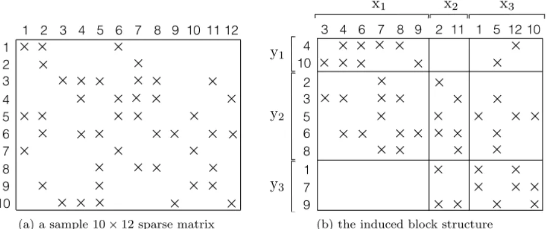
Pk or P`. Figure 6 illustrates a sample 10×12 sparse matrix and its block structure
induced by a sample 3-way vector distribution which incurs four messages: from P3
to P1, from P1 to P2, from P3 to P2, and from P2 to P3 due to A13, A21, A23, and
A32, respectively.
Since diagonal blocks and zero off-diagonal blocks do not incur any communica-tion, we focus on the nonzero off-diagonal blocks. Consider a nonzero off-diagonal block Ak` which incurs a message from P` to Pk. The volume of this message is
determined by the distribution of tasks of Ak` between Pk and P`. This in turn
im-plies that distributing the tasks of each nonzero off-diagonal block can be performed independently for minimizing the total communication volume.
C36 E. KAYAASLAN, C. AYKANAT, AND B. UC¸ AR 2 2 2 2 2 2 2 3 3 3 2 2 2 2 2 3 3 3 3 3 3 3 3 1 1 1 2 2 2 2 1 1 2 1 2 2 2 3 5 6 8 3 4 6 7 8 9 4 10 1 7 9 2 11 1 5 10 x1 x2 x3
y
1y
2y
3 12 2 9 1 7 4 10 6 8 3 5 11 6 10 3 4 5 7 8 9 2 1 12 2 3 5 6 8 3 4 6 7 8 9 4 10 1 7 9 2 11 1 5 10x
1x
2x
3y
1y
2y
3 12 1 1 1 1 1 1 1 1 2 2 2 2 2 2 3 3 3 3 2 2 2 3 3 3 3 3 3 3 3 3 3 3 1 1 1 1 1 1 2 2 2 2 2 2 2 3 5 6 8 3 4 6 7 8 9 4 10 1 7 9 2 11 1 5 10x
1x
2x
3y
1y
2y
3 12 1 1 1 1 1 1 1 1(a) a sample 10 × 12 sparse matrix
2 2 2 2 2 2 2 3 3 3 2 2 2 2 2 3 3 3 3 3 3 3 3 1 1 1 2 2 2 2 1 1 2 1 2 2 2 3 5 6 8 3 4 6 7 8 9 4 10 1 7 9 2 11 1 5 10 x1 x2 x3
y
1y
2y
3 12 2 9 1 7 4 10 6 8 3 5 11 6 10 3 4 5 7 8 9 2 1 12 2 3 5 6 8 3 4 6 7 8 9 4 10 1 7 9 2 11 1 5 10x
1x
2x
3y
1y
2y
3 12 1 1 1 1 1 1 1 1 2 2 2 2 2 2 3 3 3 3 2 2 2 3 3 3 3 3 3 3 3 3 3 3 1 1 1 1 1 1 2 2 2 2 2 2 2 3 5 6 8 3 4 6 7 8 9 4 10 1 7 9 2 11 1 5 10x
1x
2x
3y
1y
2y
3 12 1 1 1 1 1 1 1 1(b) the induced block structure
Fig. 6. A sample 10 × 12 sparse matrix A and its block structure induced by input-data dis-tribution Π(x) = {x(1), x(2), x(3)} and output-data distribution Π(y) = {y(1), y(2), y(3)}, where x(1) = {x
3, x4, x6, x7, x8, x9}, x(2) = {x2, x11}, x(3) = {x1, x5, x12, x10}, y(1) = {y4, y10}, y(2)= {y
2, y3, y5, y6, y8}, and y(3)= {y1, y7, y9}.
In the local row-column-parallel algorithm, P`sends [ˆx(k)` , ˆy (`)
k ] to Pk. Here, ˆx(k)`
corresponds to the nonzero columns of A(`)`k, and ˆyk(`)corresponds to the nonzero rows of A(k)`k for a nonzero/task distribution Ak` = A(k)k` + A
(`)
k`. Then we can derive the
following formula for the communication volume φk`from P` to Pk:
(12) φk`= ˆn(A(k)k`) + ˆm(A
(`)
k`),
where ˆn(·) and ˆm(·) refer to the number of nonzero columns and nonzero rows of the input submatrix, respectively. The total communication volume φ is then com-puted by summing the communication volumes incurred by each nonzero off-diagonal block of the block structure. Then the problem of our interest can be described as follows.
Problem 4.1. Given A and a vector distribution (Π(x), Π(y)), find a nonzero/ task distribution Π(A) such that (i) each nonzero off-diagonal block has the form Ak`= A(k)k` + A
(`)
k`, (ii) each diagonal block Akk= A(k)kk in the block structure induced
by(Π(x), Π(y)), and (iii) the total communication volume φ =P
k6=`φk`is minimized.
Let Gk` = (Uk`∪ Vk`, Ek`) be the bipartite graph representation of Ak`, where
Uk` and Vk` are the set of vertices corresponding to the rows and columns of Ak`,
respectively, and Ek`is the set of edges corresponding to the nonzeros of Ak`. Based
on this notation, the following theorem states a correspondence between the problem of distributing nonzeros/tasks of Ak`to minimize the communication volume φk`from
P` to Pk and the problem of finding a minimum vertex cover of Gk`. Before stating
the theorem, we give a brief definition of vertex covers for the sake of completeness. A subset of vertices of a graph is called vertex cover if each of the graph edges is incident to any of the vertices in this subset. A vertex cover is minimum if its size is the least possible. In bipartite graphs, the problem of finding a minimum vertex cover is equivalent to the problem of finding a maximum matching [13]. Aschraft and Liu [1] describe a similar application of vertex covers.
Theorem 4.2. Let Ak`be a nonzero off-diagonal block andGk`= (Uk`∪Vk`,Ek`)
be its bipartite graph representation:
1.5D PARALLEL SPARSE MATRIX-VECTOR MULTIPLY C37 1. For any vertex cover Sk`ofGk`, there is a nonzero distribution Ak`= A(k)k` +
A(`)k` such that|Sk`| ≥ ˆn(A(k)k`) + ˆm(A(`)k`);
2. For any nonzero distribution Ak`= A(k)k` + A (`)
k`, there is a vertex coverSk`
of Gk`such that |Sk`| = ˆn(A(k)k`) + ˆm(A(`)k`).
Proof. We prove the two parts of the theorem separately.
1) Take any vertex cover Sk` of Gk`. Consider any nonzero distribution Ak`=
A(k)k` + A(`)k` such that (13) aij ∈ A(k)k` if vj∈ Sk`and ui6∈ Sk`, A(`)k` if vj6∈ Sk`and ui∈ Sk`, A(k)k` or A(`)k` if vj∈ S`and ui∈ Sk`.
Since vj ∈ Sk` for every aij ∈ A(k)k` and ui ∈ Sk` for every aij ∈ A(`)k`,
|Sk`∩ Vk`| ≥ ˆn(A(k)k`) and|Sk`∩ Uk`| ≥ ˆm(A(`)k`), which in turn leads to
|Sk`| ≥ ˆn(A(k)k`) + ˆm(A (`)
k`).
(14)
2) Take any nonzero distribution Ak`= A(k)k` + A(`)k`. Consider Sk`={ui∈ Uk`:
aij ∈ A(`)k`} ∪ {vj ∈ Vk`: aij ∈ A(k)k`}, where |Sk`| = ˆn(A(k)k`) + ˆm(A (`) k`). Now
consider a nonzero aij ∈ Ak` and its corresponding edge {ui, vj} ∈ Ek`. If
aij ∈ A(k)k`, then vj∈ Sk`. Otherwise, ui∈ Sk`since aij ∈ A(`)k`. So, Sk`is a
vertex cover of Gk`.
At this point, however, it is still not clear how the reduction from the problem of distributing the nonzeros/tasks to the problem of finding the minimum vertex cover holds. For this purpose, using Theorem 4.2, we show that a minimum vertex cover of Gk` can be decoded as a nonzero distribution of Ak` with the minimum
communication volume φk`as follows. Let Sk`∗ be a minimum vertex cover of Gk`and
φ∗
k` be the minimum communication volume incurred by a nonzero/task distribution
of Ak`. Then|Sk`∗ | = φ∗k`since the first and second parts of Theorem 4.2 imply|Sk`∗| ≥
φ∗
k` and |Sk`∗| ≤ φ∗k`, respectively. We decode an optimal nonzero/task distribution
Ak`= A(k)k` + A (`)
k` out of Sk`∗ according to (13), where one such distribution is
(15) A(k)k` ={aij∈ Ak`: vj ∈ Sk`∗} and A (`)
k` ={aij ∈ Ak`: vj 6∈ S
∗
k`}.
Let φk` be the communication volume incurred by this nonzero/task distribution.
Then, |S∗
k`| ≥ φk` due to (14), and φk`= φ∗k`since φk`∗ =|Sk`∗ | ≥ φk`≥ φ∗k`.
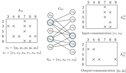
Figure 7 illustrates the reduction on a sample 5×6 nonzero off-diagonal block Ak`.
The left side and middle of this figure, respectively, display Ak`and its bipartite graph
representation Gk`, which contains five row vertices and six column vertices. In the
middle of the figure, a minimum vertex cover Sk` that contains two row vertices
{u3, u6} and two column vertices {v7, v8} is also shown. The right side of the figure
displays how this minimum vertex cover is decoded as a nonzero/task distribution Ak` = A(k)k` + A
(`)
k`. As a result of this decoding, P` sends [x7, x8, ˆy3, ˆy6] to Pk in a
single message. Note that a nonzero corresponding to an edge connecting two cover vertices can be assigned to either A(k)k` or A(`)k` without changing the communication volume from P` to Pk. The only change that may occur is in the values of partially
computed output-vector entries to be communicated. For instance, in the figure,
C38 E. KAYAASLAN, C. AYKANAT, AND B. UC¸ AR u2 u3 u5 u8 v3 v4 v6 v7 v8 v9 u6 Sk`={u3, u6, v7, v8} Gk` Ak` 2 3 5 6 8 3 4 6 7 8 9 yk={y2, y3, y5, y6, y8} x`={x3, x4, x6, x7, x8, x9} 2 3 5 6 8 3 4 6 7 8 9 A(`)k` Output-communication [ˆy3, ˆy6] A(k)k` 2 3 5 6 8 3 4 6 7 8 9 Input-communication [x7, x8]
Fig. 7. The minimum vertex cover model for minimizing the communication volume φk`from P`to Pk. According to the vertex cover Sk`, P`sends [x7, x8, ˆy3, ˆy6] to Pk.
nonzero a37is assigned to A(k)k`. Since both u3and v7are cover vertices, a37could be
assigned to A(`)k` with no change in the communicated entries but the value of ˆy3.
Algorithm 3 gives a sketch of our method to find a nonzero/task distribution that minimizes the total communication volume based on Theorem 4.2. For each nonzero off-diagonal block Ak`, the algorithm first constructs Gk`, then obtains a
minimum vertex cover Sk`, and then decodes Sk` as a nonzero/task distribution
Ak` = A(k)k` + A(`)k` according to (15). Hence, the communication volume incurred
by Ak` is equal to the size of the cover|Sk`|. In detail, each row vertex ui on the
cover incurs an output communication of ˆyi ∈ ˆy`(k), and each column vertex vj on
the cover incurs an input communication of xj ∈ ˆx(`)k . We recall that P` sends ˆy(k)`
and ˆx(`)k to Pkin a single message in the proposed row-column-parallel sparse
matrix-vector multiply algorithm.
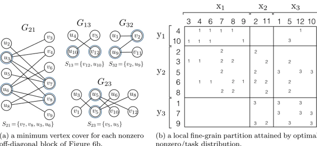
Figure 8 illustrates the steps of Algorithm 3 on the block structure given in Figure 6(b). Figure 8(a) shows four bipartite graphs each corresponding to a nonzero off-diagonal block. In this figure, a minimum vertex cover for each bipartite graph is also shown. Figure 8(b) illustrates how to decode a local fine-grain partition from those minimum vertex covers. In this figure, the nonzeros are represented with the processor to which they are assigned. As seen in the figure, the number of entries sent
Algorithm 3. Nonzero/task distribution to minimize the total communication volume.
1: procedure NonzeroTaskDistributeVolume(A, Π(x), Π(y))
2: for eachnonzero off-diagonal block Ak`do I See (3)
3: Construct Gk`= (Uk`∪ Vk`,Ek`) I Bipartite graph representation
4: Sk`← MinimumVertexCover(Gk`)
5: for eachnonzero aij ∈ Ak`do
6: if vj∈ Sk`then I vj ∈ Vk`is a column vertex and vj∈ Sk`
7: A(k)k` ← A(k)k` ∪ {aij}
8: else I ui∈ Uk`is a row vertex and ui∈ Sk`
9: A(`)k` ← A(`)k` ∪ {aij}
1.5D PARALLEL SPARSE MATRIX-VECTOR MULTIPLY C39 u2 u3 u5 u8 v3 v4 v6 v7 v8 v9 u6
G
21G
13 v12 v5 u4 u10G
32 v2 v11 u1 u9G
23 v5 v1 v10 v12 u3 u5 u6 u8S21={v7, v8, u3, u6} S23={v5, u5}
S13={v12, u10} S32={v2, u9}
(a) a minimum vertex cover for each nonzero off-diagonal block of Figure 6b.
2 3 5 6 8 3 4 6 7 8 9 4 10 1 7 9 2 11 1 5 10 x1 x2 x3
y
1y
2y
3 12 2 9 1 7 4 10 6 8 3 5 11 6 10 3 4 5 7 8 9 2 1 12 2 3 5 6 8 3 4 6 7 8 9 4 10 1 7 9 2 11 1 5 10x
1x
2x
3y
1y
2y
3 12 2 2 2 2 2 2 3 3 3 3 3 2 2 2 2 3 3 3 3 3 3 3 3 3 1 1 1 1 1 1 1 2 2 2 2 2 2 3 5 6 8 3 4 6 7 8 9 4 10 1 7 9 2 11 1 5 10x
1x
2x
3y
1y
2y
3 12 1 1 1 1 1 1 1 1 2 2 2 2 2 2 2 3 3 3 2 2 3 3 2 3 3 3 3 3 3 3 3 1 1 1 2 2 2 2 1 1 2 1 2 2 1 1 1 1 1 1 1 1(b) a local fine-grain partition attained by optimal nonzero/task distribution.
Fig. 8. An optimal nonzero distribution minimizing the total communication volume obtained by Algorithm 3. The matrix nonzeros are represented with the processors they are assigned to. The total communication volume is 10, where P1 sends [x7, x8, ˆy3, ˆy6] to P2, P3 sends [x12, ˆy10] to P1, P3 sends [x2, ˆy9] to P1, and P3 sends [x5, ˆy5] to P2.
from P1 to P2 is four, that is, φ21= 4, and the number of entries sent from P3to P1,
from P3 to P2 and from P2to P3 are all two, that is, φ13= φ23= φ32= 2.
We note here that the objective of this method is to minimize the total com-munication volume under a given vector distribution. Since blocks of nonzeros are assigned, a strict load balance cannot be always maintained.
5. Related work. Here we review recent related work on matrix partitioning for parallel SpMV.
Kuhlemann and Vassilevski [14] recognize the need to reduce the number of mes-sages in parallel sparse matrix vector multiply operations with matrices corresponding to scale-free graphs. They present methods to embed the given graph in a bigger one to reduce the number of messages. The gist of the method is to split a vertex into a number of copies (the number is determined with a simple calculation to limit the maximum number of messages per processor). In such a setting, the SpMV opera-tions with the matrix associated with the original graph, y←Ax, is then cast as triple sparse matrix vector products of the form y← QT(B(Qx)). This original work can
be extended to other matrices (not necessarily symmetric or square) by recognizing the triplet product as a communication on x for duplication (for the columns that are split), communication of x vector entries (duplicates are associated with different destinations), multiplication, and a communication on the output vector (for the rows that are split) to gather results. This exciting extension requires further analysis.
Boman et al. [2] propose a 2D partitioning method obtained by postprocessing a 1D partition. Given a 1D partition among P processors, the method maps the P× P block structure to a virtual mesh of size Pr× Pc and reassigns the off-diagonal blocks
so as to limit the number of messages per processor by Pr+ Pc. The postprocessing
is fast, and hence the method is nearly as efficient as a 1D partitioning method. However, the communication volume and the computational load balance obtained in the 1D partitioning phase are disturbed, and the method does not have any means to control the perturbation. The proposed two-part method (section 4.2) is similar to this work in this aspect; a strict balance cannot always be achieved, yet a finer approach is discussed in the preliminary version of the paper [12].
C40 E. KAYAASLAN, C. AYKANAT, AND B. UC¸ AR
Pelt and Bisseling [15] propose a model to partition sparse matrices into two parts (which then can be used recursively to partition into any number of parts). The essential idea has two steps. First, the nonzeros of a given matrix A are split into two different matrices (of the same size as the original matrix), say, A = Ar+ Ac.
Second, Ar and Ac are partitioned together, where Ar is partitioned row-wise and
Ac is partitioned column-wise. As all nonzeros of A are in only one of Aror Ac, the
final result is a 2-way partitioning of the nonzeros of A. The resulting partition on A achieves load balance and reduces the total communication volume by the standard hypergraph partitioning techniques.
2D partitioning methods that bound the maximum number of messages per processor, such as the checkerboard-[5, 8] and orthogonal recursive bisection [17]– based methods, have been used in modern applications [18, 20], sometimes without graph/hypergraph partitioning [19]. In almost all cases, inadequacy of 1D partitioning schemes are confirmed.
All previous work (including those that were summarized above) assumes the standard SpMV algorithm based on expanding x-vector entries, performing multiplies with matrix entries, and folding y-vector entries. Compared to all these previous works, ours has therefore a distinctive characteristic. In this work, we introduce the novel concept of heterogeneous messages where x-vector and partially computed y-vector entries are possibly communicated within the same message packet. In order to make use of this, we search for a special 2D partition on the matrix nonzeros in which a nonzero is assigned to a processor holding either the associated input-vector entry, the associated output-vector entry, or both. The implication is that the proposed local row-column-parallel SpMV algorithm requires only a single communication phase (all the previous algorithms based on 2D partitions require two communication phases) as is the case for the parallel algorithms based on 1D partitions, yet the proposed algorithm achieves a greater flexibility to reduce the communication volume than the 1D methods.
6. Experiments. We performed our experiments on a large selection of sparse matrices obtained from the University of Florida (UFL) sparse matrix collection [9]. We used square and structurally symmetric matrices with 500–10M nonzeros. At the time of experiments, we had 904 such matrices. We discarded 14 matrices, as they contain diagonal entries only, and we also excluded one matrix (kron g500-logn16) because it took extremely long to have a partition with the hypergraph partitioning tool used in the experiments. We conducted our experiments for K = 64 and K = 1024 and omit the cases when the number of rows is less than 50× K. As a result, we had 566 and 168 matrices for the experiments with K = 64 and 1024, respectively. We separate all our test matrices into two groups according to the maximum number of nonzeros per row/column, more precisely, according to whether the test matrix contains a dense row/column or not. We say a row/column dense if it contains at least 10√m nonzeros, where m denotes the number of rows/columns. Hence, for K = 64 and 1024, the first group contains, respectively, 477 and 142 matrices, which have no dense rows/columns out of 566 and 168 test matrices. The second group contains the remaining 89 and 26 matrices, each having some dense rows/column, for K = 64 and 1024, respectively.
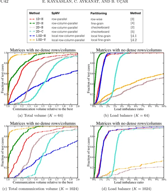
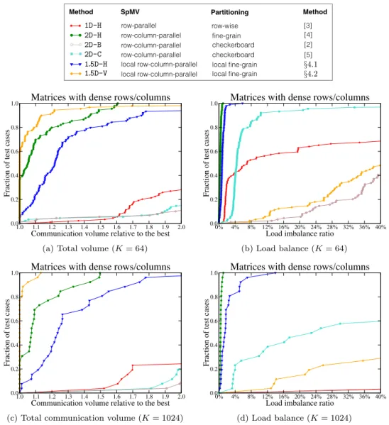
In the experiments, we evaluated the partitioning qualities of the local fine-grain partitioning methods proposed in section 4 against 1D row-wise (1D-H [3]), the 2D fine-grain (2D-H [4]), and two checkerboard partitioning methods (2D-B [2], 2D-C [5]). For the method proposed in section 4.1, we obtain a local fine-grain partition through the directed hypergraph model (1.5D-H) using the procedure described at the end of
1.5D PARALLEL SPARSE MATRIX-VECTOR MULTIPLY C41 that subsection. For the method proposed in section 4.2 (1.5D-V), the required vector distribution is obtained by 1D row-wise partitioning using the column-net hypergraph model. Then we obtain a local fine-grain partition on this vector distribution with a nonzero/task distribution that minimizes the total communication volume.
The 1D-H, 2D-H, 2D-C, and 1.5D-H methods are based on hypergraph models. Al-though all these models allow arbitrary distribution of the input- and output-vectors, in the experiments, we consider conformal partitioning of input- and output-vectors, by using vertex amalgamation of the input- and output-vector entries [16]. We used PaToH [3, 6] with default parameters where the maximum allowable imbalance ratio is 3% for partitioning. We also notice that the 1.5D-V and 2D-B methods are based on 1D-H and keep the vector distribution obtained from 1D-H intact. Hence, in the experiments, the input- and output-vectors for those methods are conformal as well. Finally, since PaToH depends on randomization, we report the geometric mean of 10 different runs for each partitioning instance.
In all experiments, we report the results using performance profiles [10], which is very helpful in comparing multiple methods over a large collection of test cases. In a performance profile, we compare methods according to the best performing method for each test case and measure in what fraction of the test cases a method performs within a factor of the best observed performance. For example, a point (abscissa = 1.05, ordinate = 0.30) on the performance curve of a given method refers to the fact that for 30% of the test cases, the method performs within a factor of 1.05 of the best observed performance. As a result, a method that is closer to top-left corner is better. In the load balancing performance profiles displayed in Figures 9(b), 9(d), 10(b), and 10(d), we compare performance results with respect to the performance of perfect balance instead of best observed performance. That is, a point (abscissa = 6%, ordinate = 0.40) on the performance curve of a given method means that for 40% of the test cases, the method produces a load imbalance ratio less than or equal to 6%.
Figures 9 and 10 both display performance profiles of four task-and-data distri-bution methods in terms of the total communication volume and the computational load imbalance. Figure 9 displays performance profiles for the set of matrices with no dense rows/columns, whereas Figure 10 displays performance profiles for the set of matrices containing dense rows/columns.
As seen in Figure 9, for the set of matrices with no dense rows/columns, the relative performances of all methods are similar for K = 64 and K = 1024 in terms of both communication volume and load imbalance. As seen in Figure 9(a) and 9(c), all methods except the 1.5D-H method achieve a total communication volume at most 30% more than the best in almost 80% of the cases in this set of matrices. As seen in these two figures, the proposed 1.5D-V method performs significantly better than all other methods, whereas the 2D-H method is the second best performing method. As also seen in the figures, 1D-H displays the third best performance, whereas 1.5D-H shows the worst performance. As seen in Figure 9(b) and 9(d), in terms of load balance, the 2D-H method is the best performing method. As also seen in the figures, the proposed 1.5D-V method displays considerably worse performance than the others. Specifically, all methods except 1.5D-V achieve a load imbalance below 3% in almost all test cases. In terms of the total communication volume, 2D checkerboard partitioning methods perform considerably worse than 1.5D-V, 2D-H and 1D-H methods. The first alternative 2D-B obtains better results than 2D-C. For load balance, 2D-C behaves similar to 1D-H, 2D-H, and 1.5D-H methods, except that 2D-C achieves a load imbalance below 5% (instead of 3%) for almost all instances. 2D-B behaves similarly to 1.5D-V and does not achieve a good load balance.
C42 E. KAYAASLAN, C. AYKANAT, AND B. UC¸ AR SpMV Partitioning Method Method 1D 2D 1.5D 1.5D-V 1.5D-L Matrices with or without dense rows (K = 1024)
local row-column-parallel 1.5D-H §4.1 1D 2D 1.5D 1.5D-V 1.5D-L Matrices with or without dense rows (K = 1024)
local row-column-parallel 1.5D-V §4.2 1D 2D 1.5D 1.5D-V 1.5D-L Matrices with or without dense rows (K = 1024)
row-parallel row-wise [3] 1D 2D 1.5D 1.5D-V 1.5D-L Matrices with or without dense rows (K = 1024)
row-column-parallel [4] row-column-parallel checkerboard [5] row-column-parallel checkerboard [2] 1D-H 2D-H 2D-B 2D-C 1.0 1.1 1.2 1.3 1.4 1.5 1.6 1.7 1.8 1.9 2.0
Communication volume relative to the best 0.0 0.2 0.4 0.6 0.8 1.0
Fraction of test cases
Matrices with no dense rows/columns
(a) Total volume (K = 64)
0% 1% 2% 3% 4% 5% 6% 7% 8% 9% 10%
Load imbalance ratio 0.0 0.2 0.4 0.6 0.8 1.0
Fraction of test cases
Matrices with no dense rows/columns
(b) Load balance (K = 64)
1.0 1.1 1.2 1.3 1.4 1.5 1.6 1.7 1.8 1.9 2.0
Communication volume relative to the best 0.0 0.2 0.4 0.6 0.8 1.0
Fraction of test cases
Matrices with no dense rows/columns
(c) Total communication volume (K = 1024)
0% 1% 2% 3% 4% 5% 6% 7% 8% 9% 10%
Load imbalance ratio 0.0 0.2 0.4 0.6 0.8 1.0
Fraction of test cases
Matrices with no dense rows/columns
(d) Load balance (K = 1024)
Fig. 9. Performance profiles comparing the total communication volume and load balance using test matrices with no dense rows/columns for K = 64 and 1024.
As seen in Figure 10, for the set of matrices with some dense rows/columns, all methods display a similar performance for K = 64 and K = 1024 in terms of the total communication volume. As in the previous data set, in terms of the total com-munication volume, the 1.5D-V and 2D-H methods are again the best and second best methods, respectively, as seen in Figure 10(a) and 10(c). As also seen in these figures, 1.5D-His the third best performing method in terms of the total communication vol-ume, whereas 1D-H shows considerably worse performance. The 2D-H method achieves near-to-perfect load balance in almost all cases, as seen in Figure 10(b) and 10(d). As also seen in these figures, the 1.5D-H method displays a load imbalance lower than approximately 6% and 14% for all test matrices for K = 64 and 1024, respectively. This shows the success of the vertex amalgamation procedure within the context of the directed hypergraph model described in section 4.1. As seen in Figure 10(c), the total communication volume does not exceed the best method by 40% in about 75%
1.5D PARALLEL SPARSE MATRIX-VECTOR MULTIPLY C43 SpMV Partitioning Method Method 1D 2D 1.5D 1.5D-V 1.5D-L Matrices with or without dense rows (K = 1024)
local row-column-parallel 1.5D-H §4.1 1D 2D 1.5D 1.5D-V 1.5D-L Matrices with or without dense rows (K = 1024)
local row-column-parallel 1.5D-V §4.2 1D 2D 1.5D 1.5D-V 1.5D-L Matrices with or without dense rows (K = 1024)
row-parallel row-wise [3] 1D 2D 1.5D 1.5D-V 1.5D-L Matrices with or without dense rows (K = 1024)
row-column-parallel [4] row-column-parallel checkerboard [5] row-column-parallel checkerboard [2] 1D-H 2D-H 2D-B 2D-C 1.0 1.1 1.2 1.3 1.4 1.5 1.6 1.7 1.8 1.9 2.0
Communication volume relative to the best 0.0 0.2 0.4 0.6 0.8 1.0
Fraction of test cases
Matrices with dense rows/columns
(a) Total volume (K = 64)
0% 4% 8% 12% 16% 20% 24% 28% 32% 36% 40%
Load imbalance ratio 0.0 0.2 0.4 0.6 0.8 1.0
Fraction of test cases
Matrices with dense rows/columns
(b) Load balance (K = 64)
1.0 1.1 1.2 1.3 1.4 1.5 1.6 1.7 1.8 1.9 2.0
Communication volume relative to the best 0.0 0.2 0.4 0.6 0.8 1.0
Fraction of test cases
Matrices with dense rows/columns
(c) Total communication volume (K = 1024)
0% 4% 8% 12% 16% 20% 24% 28% 32% 36% 40%
Load imbalance ratio 0.0 0.2 0.4 0.6 0.8 1.0
Fraction of test cases
Matrices with dense rows/columns
(d) Load balance (K = 1024)
Fig. 10. Performance profiles comparing the total communication volume and the load balance on test matrices with dense rows/columns for K = 64 and 1024.
and 85% of the test cases for the 1.5D-H and 2D-H methods, respectively, for K = 1024. The two 2D checkerboard methods display considerably worse performance than the others (except 1D-H, which also shows a poor performance) in terms of the total com-munication volume. When K = 64, 2D-C shows an acceptable performance; however, when K = 1024, its performance considerably deteriorates in terms of load balance. 2D-B obtains worse results. This not surprising since 2D-B is a modification of 1D-H, whose load balance performance is already very poor.
Figure 11(a) and 11(b) compares the methods in terms of the total and maximum message counts, respectively, using all test matrices for K = 1024. We note that these are secondary metrics, and none of the methods addresses them explicitly as the main objective function. Since 1.5D-V uses the conformal distribution of the input- and output-vectors obtained from 1D-H, the total and the maximum message counts of 1.5D-V are equivalent to those of 1D-H in these experiments. As seen in the figure,
C44 E. KAYAASLAN, C. AYKANAT, AND B. UC¸ AR SpMV Partitioning Method Method 1D 2D 1.5D 1.5D-V 1.5D-L Matrices with or without dense rows (K = 1024)
local row-column-parallel 1.5D-H §4.1 1D 2D 1.5D 1.5D-V 1.5D-L Matrices with or without dense rows (K = 1024)
local row-column-parallel 1.5D-V §4.2 1D 2D 1.5D 1.5D-V 1.5D-L Matrices with or without dense rows (K = 1024)
row-parallel row-wise [3] 1D 2D 1.5D 1.5D-V 1.5D-L Matrices with or without dense rows (K = 1024)
row-column-parallel [4] row-column-parallel checkerboard [5] row-column-parallel checkerboard [2] 1D-H 2D-H 2D-B 2D-C 1.0 1.1 1.2 1.3 1.4 1.5 1.6 1.7 1.8 1.9 2.0
Number of messages relative to the best 0.0 0.2 0.4 0.6 0.8 1.0
Fraction of test cases
All matrices
(a) Total message count
1.0 1.1 1.2 1.3 1.4 1.5 1.6 1.7 1.8 1.9 2.0
Maximum number of messages relative to the best 0.0 0.2 0.4 0.6 0.8 1.0
Fraction of test cases
All matrices
(b) Maximum message count
1.0 1.1 1.2 1.3 1.4 1.5 1.6 1.7 1.8 1.9 2.0
Maximum communication volume relative to the best 0.0 0.2 0.4 0.6 0.8 1.0
Fraction of test cases
All matrices
(c) Maximum volume
1.0 1.2 1.4 1.6 1.8 2.0 2.2 2.4 2.6 2.8 3.0
Partitioning time relative to the best 0.0 0.2 0.4 0.6 0.8 1.0
Fraction of test cases
All matrices
(d) Partitioning time
Fig. 11. Performance profiles comparing the total message count and the maximum message count for three methods, 1D-H, 2D-H, and 1.5D-H; maximum communication volume per processor; and partitioning time for all methods on all test matrices for K = 1024. In 11(a) and 11(b), 1.5D-V’s profiles are identical to those of 1D-H and hence are not shown.
in terms of the total and the maximum message counts, 2D-B, 2D-C, and 1D-H (also 1.5D-V) display the best performance, 2D-H performs considerably poor, and 1.5D-H performs in between. At a finer look, the method 2D-B is the winner with both metrics. 1.5D-V (as 1D-H) and the other checkerboard method 2D-C follows it, where 2D checkerboard methods show a clearer advantage.
Figure 11(c) compares all four methods in terms of the maximum communication volume sent from a processor for K = 1024. The 1.5D-V method performs significantly better than all others, 2D-H is the second best performing method, 1D displays the third best, and 1.5D-H displays the worst performance. These relative performances of the methods in terms of the maximum communication volume resemble their relative performances in terms of the total communication volume as expected.
1.5D PARALLEL SPARSE MATRIX-VECTOR MULTIPLY C45 Figure 11(d) compares the methods in terms of partitioning times for K = 1024. The run time of the 1.5D-V method involves the time spent for obtaining the vec-tor distribution, which is the run time of the 1D-H method in our case. As seen in the figure, the 1D-H, 1.5D-V, and 1.5D-H methods display comparable performances, whereas the 2D-H method takes significantly longer. The longer run time of 2D-H stems from the large size of the hypergraph model. 2D-B displays comparable perfor-mance (in terms of running time) with that of the 1D-H, 1.5D-V, and 1.5D-H methods. Meanwhile, 2D-C is considerably slower than all others except 2D-H.
In summary, the 1.5D-H method is a promising alternative for sparse matrices with dense rows/columns. It obtains a total communication volume close to 2D-H, near-perfect balance, and a considerably lower message count than 2D-H and has short partitioning time. The 1.5D-V method performs at the extremes: the best for the total communication volume and the worst for the load balance, especially for matrices with dense rows/columns. Nevertheless, 1.5D-V could still be favorable to other methods for particular matrices due to lower communication volume. In short, if a sparse matrix contains dense rows/columns, then 1.5D-H seems to be the method of choice in general; otherwise, 1.5D-V and 1D-H are reasonable alternatives compet-ing with each other. The 2D checkerboard-based methods perform worse than the 1.5D methods, but they have good performance in terms of the message count–based metrics. In particular, 2D-B is a fast method with a striking performance in reducing the latency, but load balance can be an issue. These could be deciding factors for large-scale systems. On the other hand, 2D-C obtains better balance than 2D-B but is slower.
7. Conclusion and further discussion. This paper introduced 1.5D paral-lelism for SpMV operations. We presented the local row-column parallel SpMV that uses this novel parallelism. This multiply algorithm is the fourth one in the literature for SpMV in addition to the well-known 1D row-parallel, 1D column-parallel, and 2D row-column-parallel ones. In this paper, we also proposed two methods (1.5D-H and 1.5D-V) to distribute tasks and data in accordance with the requirements of the proposed 1.5D parallel algorithm. Using a large set of matrices from the UFL sparse matrix collection, we compared the partitioning qualities of these two methods against the standard 1D and 2D methods.
The experiments suggest the use of the local row-column-parallel SpMV with a local fine-grain partition obtained by the proposed directed hypergraph model for matrices with dense rows/columns. This is because the performance of the proposed 1.5D partitioning is close to that of 2D fine-grain partitioning (2D-H) in terms of the partitioning quality, with a considerably fewer number of messages and much faster execution.
We considered the problem mainly from a theoretical point of interest and leave the performance of 1.5D parallel SpMV algorithms in terms of the parallel multiply timings as a future work. We note that the main ideas behind the proposed 1.5D parallelism, such as heterogeneous messaging and avoiding nonlocal tasks by a locality constraint on partitioning, are of course not restricted to the parallel SpMV operation, and these ideas can be extended to other parallel computations as well.
REFERENCES
[1] C. Ashcraft and J. W. H. Liu, Applications of the Dulmage-Mendelsohn decomposition and network flow to graph bisection improvement, SIAM J. Matrix Anal. Appl., 19 (1998), pp. 325–354.
C46 E. KAYAASLAN, C. AYKANAT, AND B. UC¸ AR
[2] E. G. Boman, K. D. Devine, and S. Rajamanickam, Scalable matrix computations on large scale-free graphs using 2d graph partitioning, in Proceedings of the International Conference on High Performance Computing, Networking, Storage and Analysis, SC ’13, ACM, New York, 2013, pp. 50:1–50:12.
[3] ¨U. C¸ ataly¨urek and C. Aykanat, Hypergraph-partitioning-based decomposition for paral-lel sparse-matrix vector multiplication, IEEE Trans. Paralparal-lel Distrib. Syst., 10 (1999), pp. 673–693.
[4] ¨U. C¸ ataly¨urek and C. Aykanat, A fine-grain hypergraph model for 2d decomposition of sparse matrices, in Proceedings of the International Parallel and Distributed Processing Symposium, Vol. 3, IEEE Computer Society, San Francisco, CA, 2001, p. 30118b. [5] ¨U. C¸ ataly¨urek and C. Aykanat, A hypergraph-partitioning approach for coarse-grain
decom-position, in Supercomputing, ACM/IEEE 2001 Conference, IEEE, Piscataway, NJ, 2001, p. 42.
[6] ¨U. C¸ ataly¨urek and C. Aykanat, Patoh (partitioning tool for hypergraphs), in Encyclopedia of Parallel Computing, Springer, Berlin, 2011, pp. 1479–1487.
[7] ¨U. C¸ ataly¨urek, C. Aykanat, and B. Uc¸ar, On two-dimensional sparse matrix partitioning: Models, methods, and a recipe, SIAM J. Sci. Comput., 32 (2010), pp. 656–683.
[8] ¨U. V. C¸ ataly¨urek, C. Aykanat, and B. Uc¸ar, On two-dimensional sparse matrix partition-ing: Models, methods, and a recipe, SIAM J. Sci. Comput., 32 (2010), pp. 656–683. [9] T. A. Davis and Y. Hu, The University of Florida sparse matrix collection, ACM Trans. Math.
Softw., 38 (2011), pp. 1:1–1:25.
[10] E. D. Dolan and J. J. Mor´e, Benchmarking optimization software with performance profiles, Math. Program., 91 (2002), pp. 201–213.
[11] K. Kaya, B. Uc¸ar, and U. V. C¸ ataly¨urek, Analysis of partitioning models and metrics in parallel sparse matrix-vector multiplication, in Parallel Processing and Applied Mathemat-ics (PPAM2014), R. Wyrzykowski, J. Dongarra, K. Karczewski, and J. Wa´sniewski, eds., Lecture Notes in Computer Science, Warsaw, 2014, Springer, Berlin, pp. 174–184. [12] E. Kayaaslan, B. Uc¸ar, and C. Aykanat, Semi-two-dimensional partitioning for
par-allel sparse matrix-vector multiplication, in Parpar-allel and Distributed Processing Sym-posium Workshop (IPDPSW), 2015 IEEE International, IEEE, Piscataway, NJ, 2015, pp. 1125–1134.
[13] D. Konig, Gr´afok ´es m´atrixok. Mat. Fiz. Lapok, 38 (1931), pp. 116–119.
[14] V. Kuhlemann and P. S. Vassilevski, Improving the communication pattern in matrix-vector operations for large scale-free graphs by disaggregation, SIAM J. Sci. Comput., 35 (2013), pp. S465–S486.
[15] D. M. Pelt and R. H. Bisseling, A medium-grain method for fast 2d bipartitioning of sparse matrices, in Parallel and Distributed Processing Symposium, 2014 IEEE 28th International, IEEE, Piscataway, NJ, 2014, pp. 529–539.
[16] B. Uc¸ar and C. Aykanat, Revisiting hypergraph models for sparse matrix partitioning, SIAM Rev., 49 (2007), pp. 595–603.
[17] B. Vastenhouw and R. H. Bisseling, A two-dimensional data distribution method for parallel sparse matrix-vector multiplication, SIAM Rev., 47 (2005), pp. 67–95.
[18] R. S. Xin, J. E. Gonzalez, M. J. Franklin, and I. Stoica, Graphx: A resilient distributed graph system on spark, in First International Workshop on Graph Data Management Ex-periences and Systems, GRADES ’13, ACM, New York, 2013, pp. 2:1–2:6.
[19] A. Yoo, A. H. Baker, R. Pearce, and V. E. Henson, A scalable eigensolver for large scale-free graphs using 2D graph partitioning, in Proceedings of the International Conference for High Performance Computing, Networking, Storage and Analysis, ACM, New York, 2011, pp. 63:1–63:11.
[20] A. Yoo, E. Chow, K. Henderson, W. McLendon, B. Hendrickson, and U. Catalyurek, A scalable distributed parallel breadth-first search algorithm on bluegene/l, in Proceedings of the 2005 ACM/IEEE Conference on Supercomputing, SC ’05, IEEE Computer Society, Washington, DC, 2005, p. 25.