Selçuk J. Appl. Math. Selçuk Journal of Vol. 7. No.2. pp. 81-90, 2006 Applied Mathematics
One Way Fixed Effect Analysis Of Variance Under Variance Hetero-geneity And A Solution Proposal
A.Fırat Özdemir and Serdar Kurt
Dokuz Eylul University, Faculty of Arts and Sciences, Department of Statistics, Kay-naklar Campus, 35160 Buca / ˙Izmir Turkey
e-mail: firat_ ozdem ir@ deu.edu.tr, serdar_ kurt@ deu.edu.tr
Summary.In the first part of this study, the results of heteroscedasticity in one way fixed effect ANOVA have been examined with a close concern on large sample approximations of treatment and error mean sum of squares and distor-tion of the distribudistor-tion of the F ratio. Second part includes the presentadistor-tion of new and simple approximation procedure which intends to create an easy and applicable alternative. The purpose of this new approximation procedure is to preserve the actual Type I error rate at a level determined by the researcher and to increase the power as well. Third part of the study consist of a simula-tion study which was implemented to compare the actual significance level and power of the new approximation, conventional F test and two other alterna-tives (Welch Test, Kruskal-Wallis Test). Finally, some recommendations about the preference of these tests for different types of experimental conditions were given.
Key words: Heteroscedasticity, B2 test, F test, Welch Test, Kruskal-Wallis
Test
1. Introduction
The purpose of analysis of variance is to test the population mean differences for statistical significance. This is accomplished by analyzing the variance of the response variable of the experiment into two parts. First one is due to random variation and second one is due to differences between population means. This relationship is shown at Eq.(1)
(1) X =1 X =1 ¡ − ¯¢ 2 = X =1 X =1 ¡ − ¯¢ 2 + X =1 ¡¯− ¯¢ 2
These two components are then used in a test procedure called F test which has a test statistics as in Eq.(2). Under the assumption ∀= 1 2
∼ ¡ 2¢ = 1 2 (2) X =1 ( ¯− ¯) −1 X =1 X =1 ( ¯− ¯)2 − = ∼ −1−
In ANOVA, variance of the distributions in which the samples are drawn should be the same to validate the underlying probability distribution of the method and to confine the errors within the desired limits. Violation of this equal-ity of variances assumption is called as heteroscedasticequal-ity in literature. In the case of heteroscedasticity, the distribution of response variable Y will be ∀ = 1 2 ∼ ¡ 2
¢
= 1 2 when the other two basic
assumptions of analysis of variance hold. There are two main results of het-eroscedasticity; distortion of the distribution of the F ratio and discrepancy between nominal and actual significance level.
1.1. Distribution of F Ratio
The numerator and denominator sums of squares of F ratio
are distributed
as weighted sum of squares of independent normal random variables with weights 2
. When the variances differ between populations these weights are unequal
and the distributions are not chi-square. By far the best article about the effect of unequal variances on the F test is Box (1954a) (G Rupert and Jr. Miller, 1986). Box developed the distribution theory for quadratic forms in the case of heteroscedasticity and applied it to the one-way classification. The ratio of mean squares is distributed approximately as 0where
(3) = − ( − 1) P =1( − ) 2 P =1 (− 1) 2 (4) 0 = ½ P =1( − ) 2 ¾2 ½ P =1 2 ¾2 + P =1( − 2 ) 4
(5) = ½ P =1 (− 1) 2 ¾2 ½ P =1 (− 1) 4 ¾
1.2. Discrepancy between nominal and actual significance level
An experimenter may wish to test the omnibus null hypothesis of equality of treatment means at nominal significance level = 0.05. But in reality this level may reach 3 or 4 times this level which is called as actual significance level because of the heterogeneity of variances problem (Wilcox et al 1986). Degree of this discrepancy depends mainly on the degree of heterogeneity of population variances and number of replications made with each treatment. To understand the effect of unequal variances on the F test, it suffices to examine the large sample case where all the n are large. (G Rupert and Jr. Miller, 1986). The
denominator mean sum of squares is converging to its expected value, which is
(6) ⎡ ⎣ 1 − X =1 X =1 (− ¯)2 ⎤ ⎦ = 1 − X =1 (− 1)2 where2
is the variance of the observations from the i’th population. Since −
=
P
=1
(− 1) , the expectation of sum of squares error is a weighted average of
the 2
and called as ¯2.The expectation of the numerator mean sum of squares
under 0 is (7) ∙ 1 −1 P =1 ¡¯− ¯¢ 2¸ =−11 ∙ P =1 ¡¯− ¢ 2 − ¡¯− ¢ 2¸ = 1 −1 ⎡ ⎣P =1 2 − =1 2 2 ⎤ ⎦ = (1−1) P =1( − )2
This quantity is a different weighted average of the 2
and called as ¯2∗. When the
n are all equal, the two weighted averages agree (¯2= ¯2∗) which means the F
ratio is centered near 1 as it should be. In this case the variance of the numerator should be controlled in order to see the effect of variance heterogeneity.
(8) ( ) = 2¯ 4 − 1 ⎡ ⎢ ⎢ ⎢ ⎣1 + ( − 2) ( − 1) P =1 ¡ 2 − ¯2 ¢ ¯ 4 2⎤ ⎥ ⎥ ⎥ ⎦
When the variances are equal the quantity in brackets in the above formula should be 1, but it obviously exceeds this when the 2
differ. Thus the actual
variance is larger than the theoretical variance (the variance where the 2 equal) and the upper tail of the distribution of the F ratio has more mass in it than anticipated by the 2−1 distribution. For an observed F ratio the actual sig-nificance level is larger than the one calculated from the tables, but numerical studies indicate that the effect is not large. This conclusion is also born out in small samples (Box,1954a, Scheffe, 1959). When the n are unequal, the effects
can be more serious. Suppose that the large 2
happen to be associated with
the large n. Then in¯2, the large 2 receive greater weight, where as in ¯2∗
the small 2
receive greater weight. The expectation of the numerator mean
squares is, therefore, less then the expectation of the denominator, and the cen-ter of the distribution of the F ratio is shifted below 1. The actual significance level is less than the one stated from the tables (nominal values). If the large 2
are associated with the small n, the shift goes in the opposite direction. The
actual significance level exceeds its nominal level without too much disparity in the variances. Falsely reporting significant results when the small samples have the larger variances is a serious worry. To balance the experiment is very crucial if it is possible. Then unequal variances and other departures from assumptions have the least effect.
2. Different Solution Approaches
Over the years, many attempts have been made to find solutions that are ro-bust in both Type I and Type II error rate performance while at the same time having nominal performance when the homogeneity of variance assumption is not violated. There are 6 main approaches proposed to solve the mentioned problem; Approximate Tests, Exact Tests, Nonparametric Tests, Data Trans-formations, Weighted Least Square Estimation Method and Robust Statistical Procedures.
2.1. A New And Simple Approximation
Consider k independent randomly sampled groups each measured on a normally distributed random variable (Y). Variances of the populations and sample size of the groups need not to be equal. Each of the k samples of size n will have
(9) ¯ = ⎡ ⎢ ⎢ ⎣ P =1 ¡ − ¯ ¢2 (− 1) ⎤ ⎥ ⎥ ⎦ 12
For each of the k samples, if we define a weight such that P =1 = 1 (10) = 1 2 ¯ P =1 Ã 1 2 ¯ !
The variance-weighted estimate of the common mean (+) of Y becomes
(11) +=
X
=1
¯
Finally, for each of the k groups a one-sample t statistics is calculated as
(12) =
¯ − +
¯
Under the usual assumptions, each of the t will be distributed as Student’s t
with = n - 1 degrees of freedom. Several of the approximation methods that
have appeared in the literature begin with the equivalent of the same derivation. After this step, this new approximation uses a normalizing transformation on each of the sample t values directly in order to transform the each t values
in to standard normal deviate z. Several normalizing transformations for the t
statistics have appeared in the literature. One of them is “Accurate Normalizing Transformations of a Student’s t Variate” Bailey B.J.R (1980). Bailey offers a locally accurate normalizing transformation which is given as follows
(13) = ± 42 + 5(22 +3) 24 42 + +(4 2 +9) 12 12 ½ µ 1 + 2 ¶¾12 (14) 2= X =1 2 = X =1 ⎛ ⎜ ⎜ ⎝ 42 + 5(22+3) 24 42 + +(4 2 +9) 12 ⎧ ⎪ ⎨ ⎪ ⎩ ⎛ ⎜ ⎝1 + ³¯ −+ ¯ ´2 ⎞ ⎟ ⎠ ⎫ ⎪ ⎬ ⎪ ⎭ 12⎞ ⎟ ⎟ ⎠ 2
will be approximately distributed 2−1. Decision rule that the tests uses is reject the null hypothesis of of equal means if B2 exceeds the 1- quantile of a
chi-square distribution with k-1 degrees of freedom. Let us call the first part of the z transformation as coefficient c, then ;
(15) = ± ½ µ 1 + 2 ¶¾12 where (16) = 4 2 + 5(22+3) 24 42 + +(4 2 +9) 12 12 then (17) 2= X =1 2 = X =1 ⎛ ⎜ ⎜ ⎝ ⎧ ⎪ ⎨ ⎪ ⎩ ⎛ ⎜ ⎝1 + ³¯ −+ ¯ ´2 ⎞ ⎟ ⎠ ⎫ ⎪ ⎬ ⎪ ⎭ 12⎞ ⎟ ⎟ ⎠ 2
can be written with the help of a table of c’s (Table1). 3. Simulation Study
Performance of the F, Welch (W), Kruskal-Wallis(KW), Alexender-Govern(AG) and new approximation (B2) procedures have been examined by means of a
simulation study. Simulated actual significance level and and power of the test have been obtained using different sample sizes and error variances for k=3, k=6 and k=9 groups by using nominal significance level 0.05. All means were equal to 0 when predicting actual significance level. Two different configurations of mean differences were used when assesing the power of the tests. The first pattern was 1 = 2, 2 = 0, 3 = 0 while the second pattern was 1 = -1, 2 = 0, 3 = 1 in which the means were equally spaced. Each configuration was executed 10000 times. All data were generated from normal distribution by using the 13’th version of statistical software MINITAB. Different experimental desings used in simulation study and all results were given in table section at the end of the paper.
4. Conclusions
Results have been interpreted according to number of treatments, number of replications and population variances. Interpretation criterion was the close-ness of the actual significance level and nominal significance level ( =0.05).
Bradley (1978) has stated that a test can said to be robust to a specific as-sumption violation if it protects actual significance level between 0.9
1.1 . This criterion is called as Bradley’s stringent criterion of robustness and
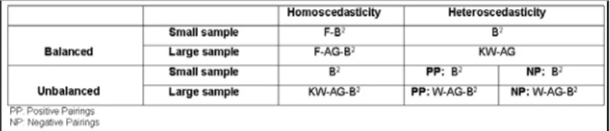
refers to 0.045 0.055 for nominal significance level of 0.05. Power values which directly change with Type I error rates have not been considered while comparing any two tests unless the actual Type I error rates of the tests are approximately equal. Power values for k=9 groups could not be given because of size problem. Recommended tests for different experimental designs were given at Table 9.
References
1. R.A. Alexender and D.M Govern, A new and Simpler Approximation for ANOVA Under Variance Heterogeneity, Journal of Educational Statistics 19, 91-101 (1994). 2. B.J.R. Bailey, Accurate Normalizing Transformations of Student’s t Variate, Ap-plied Statistics 29, 304-306 (1980).
3. G.E.P. Box, Some theorems on quadratic forms applied in the study of analysis of variance problems. Annals of Mathematical Statistics 25, 290-302 (1954a).
4. J.V. Bradley, Robustness? Brithish Journal of Mathematical and Statistical Psy-chology 31, 144-152. (1978).
5. J. Hartung, D. Argaç and K.H. Makambi, Small Sample Properties of Tests on Homogeneity in One-Way Anova and Meta-Analysis, Statistical Papers 43, 197-235. (2002).
6. W.H. Kruskal and W.A. Wallis Use of ranks in one criterion variance analysis. JASA 47, 583-621. (1952).
7. G.Rupert and J.R. Miller, Beyond ANOVA, basics of applied statistics, John Wiley & Sons. Inc Newyork (1986).
8. H. Scheffe, The Analysis of Variance, John Wiley & Sons.Inc. Newyork (1959). 9. B.L. Welch, On the comparison of several mean values, Biometrika 38, 330-336. (1951).
10. R.R. Wilcox, V.L. Charlin and K.L. Thompson, New Monte Carlo results on the robutness of the ANOVA F, W and F* statistics, Communications in Statistics: Simulation and Computation 15, 933-943. (1986).
Tables
Table 1: Coefficient of c’s up to 10 degrees of freedom for= 0.05 and= 0.01
Table 2: Sample sizes and variances of the distributions for k=3, k=6 and k=9
Table 3 : Actual significance sevels for different experimental designs of k = 3 groups
Table 5 : Actual significance levels for different experimental designs of k= 9 groups
Table 6 : Predicted power values for different experimental designs of k=3 groups
Table 8 : Codes of designs used in this simulation study