S l S P S f l ! : W 4 ,^'.f M -^r ‘!V·^ CW - ' ■'·?i>' ^ ·' ·> ^r
& 4» i - « $ W « wi 5 /à ü 4 . £ - W ■«■' A J £.· y t . “j 2 '2‘·
I
1 îâ iA THES*::
<?A
j^ û 2 - 'SALGEBRAIC THEORY OF LINEAR
MULTIVARIABLE CONTROL SYSTEMS
A THESIS
SUBMITTED TO THE DEPARTMENT OF ELECTRICAL AND ELECTRONICS ENGINEERING
AND THE INSTITUTE OF ENGINEERING AND SCIENCES OF BILKENT UNIVERSITY
IN PARTIAL FULFILLMENT OF THE REQUIREMENTS FOR THE DEGREE OF
MASTER OF SCIENCE
By
Sevgi Babacan Uetiii September 1998
ULH
4 0
Л.З. • C 4 S iSS%I certify that I have read this thesis and that in rny opinion it is fully adeciuate, in scope and in cjuality, as a thesis for the degree of Master of Science.
Prof. Dr. A. Biilent Ozguler(Supervisor)
I certify that I have recid this thesis and that in my opinion it is fully adequate, in scope and in cjuality, as a thesis for the degree of Master of Science.
rof. Dr. M. Erol Sezer
I certify that I have read this thesis and that in my opinion it is fully adequate, in scope and in quality, as a thesis for the degree of Master of Science.
Assoc. Prof. Dr. Om«i· Morgfil
Approved for the Institute of Engineering and Sciences:
Prof. Dr. Mehmet
Director of Institute of EngineeWig and Sciences
ABSTRACT
ALGEBRAIC THEORY OF LINEAR
MULTIVARIABLE CONTROL SYSTEMS
Sevgi Babacan Çetin
M .S . in Electrical and Electronics Engineering Supervisor: Prof. Dr. A . Bülent Özgüler
September 1998
The theory of linear multivariable systems stands out as tlie most devel oped and sophisticated among the topics of system theory. In the literature, many different solutions are presented to the linear midtivariable control prob lems using three main approaches : geometric approacli, fractional approach and polynomial model based approach. This thesis is a first draft for a text book on linear multivariable control which contains a description of solutions to the most of the standard algebraic feedback control problems using simple linear algebra and a minimal amount of polynomial algebra. These problems are internal stabilization, disturbance decoupling by state feedback and mea surement feedback, output stabilization, tracking with regulation in a scalar system, regulator problem with a single output channel and decentralized sta bilization.
Keywords: Multivariable control, fractional approach, internal stabilization, disturbance decoupling, tracking and regulation, decentralized stabilization.
ÖZET
Ç O K D E Ğ İŞ K E N L İ D O Ğ R U S A L K O N T R O L S İS T E M L E R İN İN C E B İR SE L T E O R İS İ
Sevgi Babacan Çetin
Elektrik ve Elektronik Mühendisliği Bölümü Yüksek Lisans Tez Yöneticisi: Prof. Dr. A . Bülent Özgüler
Eylül 1998
Çokdeğişkenli doğrusal sistemler, sistem teorisinin en karmaşık ve en fazla işlenmiş alanını oluşturmaktadır. Literatürde birçok çokdeğişkenli doğrusal sistem problemi şu üç yöntemden biri kullanılarak çözülmüştür : geometrik yaklaşım, kesir yaklaşımı ve polinom modellere dayalı yaklaşım. Çokdeğişkenli doğrusal kontrol üzerine bir ders kitabı taslağı olarak hazırlanan bu çalışma, birçok cebirsel geribeslemeli denetim probleminin çözümünü, basit doğrusal ce bir yöntemleri ve minimum miktarda polinom cebiri kullanarak sunmaktadır. Ele alınan başlıca problemler şunlardır : içsel kararlılaştırma, durum ve ölçüm geribeslemesiyle bozanetkeni ortadan kaldırma, çıktı kararlılaştırılması, sayıl bir sistemde düzenleme ile izleme, tek çıktı kanallı düzenleme problemi ve dağıtılmış (özeksiz) kararlılaştırma.
Anahtar Kelimeler: Çokdeğişkenli kontrol, kesir yaklaşımı, içsel kararlılaştırma, bozanetkeni ortadan kaldırma, düzenleme ve izleme, dağıtılmış (özeksiz) kararlılaştırma.
A C K N O W L E D G M E N T S
I would like to express my sincere gratitude to Prof. Dr. A. Bülent Özgüler for his supervision, guidance, suggestions, and especially encouragement through out the development of this thesis.
I would like to thank Prof. Dr. Erol Sezer and Assoc. Prof. Dr. Ömer Morgül for reading and commenting on the thesis.
I express my special thanks to Ismail and my parents for their constant support, patience and sincere love.
Contents
1 IN T R O D U C T IO N 1
2 LIN EAR TIM E IN V A R IA N T SYSTEM S: SOME BASIC
CON CEPTS 6
2.1
State and Output Trajectories 72.2
Stability of LTI Systems2.3 Reachability of LTI S y s te m s ... 13
2.4 Transformation of Linear S y ste m s... 17
2.5 Separation of the Reachable P a r t ... 18
2.6 Notes and R eferen ces... 21
3 STATE FEED BACK 22 3.1 Reachability and F eed b a ck ... 23
3.2 Eigenvalue A ssign m en t... 26
3.3 Stabilizability... 29
3.4 Notes and References 30
4 OBSERVABILITY A N D OBSERVERS 32
4.1 O b s e r v a b ility ... 33
4.2 Dynamic Asymptotic O b s e r v e r s ... 37
4.3 Functional Observers 40
4.4 Notes and R eferen ces... 43
5 D Y N A M IC STABILIZING CON TROLLER 44
5.1 Kalman Canonical D ecom p osition ... A5
5.2 Combined Observer and State Feedback C on trollers... 49
•5.3 Notes and R eferen ces... 52
6 F R A C T IO N A L REPRESENTATIONS 53
6.1
Right and Left Coprime Fractional R epresen tation s... .546.2 Coprime Factorization From State-Space Description .56
6.3 Common Factors and Unimodular M atrices... 59
6.4 Some Properties of Polynomial M a t r i c e s ... 62
7
ALL INTERNALLY STABILIZING CONTROLLERS
67
7.1 Closed Loop S tability...
68
7.2
Parametrization Of All Stabilizing C o n tr o lle r s ... 747..3 Strong Stabilization... 76
7.4 Notes and References 78
8 D IST U R B A N C E D ECO UPLIN G 79
8.1 A Disturbance Decoupled System 80
8.2
Disturbance Decoupling By State Feedback... 818
.2.1
Geometric A p p r o a c h ... 828
.2.2
Tran.sfer Matrix Approach 868.3 Disturbance Decoupling By Measurement F e e d b a c k ... 91
8.4 Notes and References 95
9 T R A C K IN G A N D REG U LATIO N 97
9.1 Output Stcvbilization Problem 98
9.2 Tracking with Regulation; Scalar Case 106
9.3 Regulator Problem with a Single Output C h a n n e l...109
9.4 Notes and R eferen ces...113
10 DECENTRALIZED STABILIZATION
114
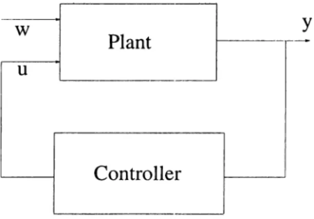
10.1 Decentralized Stabilization P ro b le m ...115
10.2 Decentralized Fixed M o d e s ...
121
10.3 Notes and R eferen ces...
122
List of Figures
2.1 Equivalence of linear systems 17
3.1 The system (
2
.1
) with state f e e d b a c k ... 234.1 Open loop system state r e c o n s tr u c tio n ... 37
5.1 Kalman d e co m p o sitio n ... 46
5.2
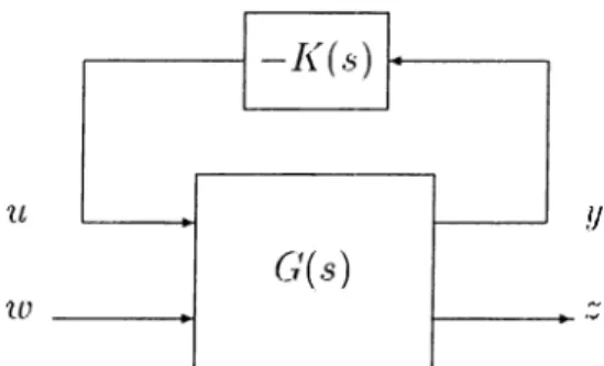
Closed loop observer plus state feedback configuration 507.1 Feedback loop for internal stability 68
8.1 Two channel system with measurement feed ba ck ... 92
9.1 Tracking with regulation 106
9.2
RPIS with a single output channel 10910.1
Closed loop system for D S P ...116Chapter 1
IN TR O D U C TIO N
The theory of linear multivariable systems stands out as the most developed and sophisticated among the topics of system theory. The structure of a multi- variable dynamic system and the limitations it may impose on the success of a feedback control applied on this system in order to satisfy certain design speci fications are well-investigated and well-understood for a large class of idealized control problems.
Yet, reference by control system designers to very basic and relevant results the tlieoiy has accumulated still remains surprisingly limited. Some quick explanations for this are that the real systems are too complex to yield to linear analysis, or that the design specifications are usually many more in number than any theory can anticipate. Such explanations can be discarded on the grounds that Newton’s theory of motion is indispensible to designers of
automobiles although an automobile is in fact far more complex than a point- mass. The reason for the limited attention the theoiy has received perhaps lies elsewhere.
If we consider one of the simplest feedback control problems of multivari able systems, say the disturbance decoupling prol)lem, then we may better understand the source of difficulty. The problem at its most generality is the following; A system with two groups of outputs and two groups of inputs are given. One group of inputs, called the disturbance inputs, consists of variables with unwanted influence on one group of outputs, called the regulated out puts. The second groups of inputs and outputs consist of the inputs available for control, called the control inputs, and the outputs that can be measured, called the measured outputs. The problem is to determine a feedback controller which processes the measured outputs to produce values for the control inputs such that in the closed loop system the disturbance inputs have no influence on the regulated outputs. Since the introduction of a feedback loop into any system may cause instabilities of the signals around the loop, the satisfaction of stability of the feedback loop is another specification on the controller to be determined. The problem is a very basic one in many disciplines where a formal model is used for describing the system at hand. The disturbance inputs sum up the variables that are external to the model which are known to influence certain states or outputs. But the dynamics with which these variables are generated the model builder has little or no knowledge of.
The multivariable control systems literature contains many different solu tions to this problem. The differences are in the language used in formulating the condition for solvability as well as in the technique of construction of a
controller whenever one exists. One class of solutions uses the language of the so-called geometric approach. The condition for solvability is formulated in terms of (A^B) and {C^A) invariant subspaces which require an advanced knowledge of linear algebra. The construction of a controller in this approach is via the construction of a state-feedback matrix F and output injection matrix K which make certain subspaces {A + 5F)-invariant and {A-\- A"C'j-invariant. The procedure is anything but straightforward. The second class of solutions uses the language of fractional approach or factorization approach. The condi tion for solvability, in its cleanest form, is formulated in terms of system ma trices and as the existence of zero-cancellations among these system matrices. The construction of a solution requires an advanced knowledge of polynomial, or alternatively stable proper rational, matrix algebra. The procedure again is not at all simple. The link between the two approaches is not always obvious. It is quite usual that the specialists in one approach cannot follow the details of construction or even cannot fully grasp the limitations imposed by the solv ability condition given by the other approach. In fact, a full exploration of the link between the two approaches is a speciality of another area of research known as the theory of polynomial models.
The picture drawn above may indeed look complicated to a researcher out side the area of control theory as well as to a designer of control systems. Although the rather heavy specialization in certain techniques is not a weak ness of a theory, the fact that each particular approach demands a sophisticated mathematical background even at the descriptive level of stating the condition for solvability does shy away the potential appliers of the theory.
Having identified the source of difficulty as such, what needs to be done is clear. The results obtained by the theory must be presented in as simple a manner as possible, eliminating the need for a sophisticated mathematical background. This thesis attempts to present some of the known solutions to a number of standard problems of multivariable control systems with this objective in mind. The proofs given for Theorems (8.2.3) and (8.2.4) of the solution to disturbance decoupling problem without and with stability and the proof given for Theorem (9.1.1) of the output stabilization problem, a proto type problem of regulation, use simple linear algeirra and a minimal amount of polynomial algebra. The link between the two solvability conditions, one com ing from geometric approach and the other from fractional approach, are made explicit without recource to the theory of polynomial models. As they stand, the results and the construction of the controllers in these theorems should be easy to follow for anyone with a basic background in linear systems. This necessary background is given in Chapters 2-5 with as little technical demand from the reader as possible. Other standard problems of linear multivariable control are also presented. These include disturbance decoupling problem with measurement feedback as posed above, regulation and tracking problems, and decentralized stabilization problem. These incorporated, the thesis is a first draft for a textbook on linear multivariable control.
The thesis is organized as follows; Chapter 2 is devoted to some basic con cepts of linear time invariant systems. Stability, reachability, equivalence of linear time invariant systems are presented. In Chapter 3, state feedback is introduced and the procedure for eigenvalue assignment is given. The concept of stabilizability also mentioned. Chapter 4 includes the concept of observabil ity and synthesis of dynamic asymptotic observers and functional observers.
In Chapter 5, Kalman Canonical Decomposition theorem is given and the sep aration principle lor feedback controllers is establihed. In Chapter
6
, stable proper factorizations are examined. Chapter 7 contains the parametrization of all controllers in terms of a free parameter. In Chapter8
, the problem of cancelling the effect of disturbances using state feedback and output measure ment feedback is examined. Two main cipproaches to this problem namely the geometric approach and the transfer matrix approach are reviewed and the so lution techniques of these two approaches are illustrated. Output stabilization, tracking and regulation problem in the scalar system and regulator problem with a single output channel is considered in Chapter 9. In Chapter10
, we show how the decentralized stabilization problem can be transformed into a “make-coprime” problem. Finally concluding remarks are given.Chapter 2
LIN EAR TIM E IN V A R IA N T
SYSTEM S: SOME BASIC
CONCEPTS
In this chapter, we shall introduce the state variable description of linear time invariant systems. Then, the definitions of equilibrium state, asymptotic and ex
23
onential stabilitj^ are given. Finally, the concept of reachability, equivalent dynamical representations and how we can sej^arate the reachcible part are presented.A linear time invariant (LTI) system is defined by a pair of equations
x{t) = Ax{t) + Bic{t), (2.1)
y{t) = Cx{t) + Du{t), t > 0 ,
where A, C , D are constant, real matrices of sizes n x n, n x m, p x ?i, p x »??., respectively. For every t > 0, x(t) G R " , u{t) E R ”', and ¡/(t) E R'h The
components iti(i), i = of u{t) are assumed to l)e piecewise continuous functions on the interval [0,oo). The vectors .r(i), ?/(/), and u{t) are called the state, output, and input of (2.1), respectively. Occasionally, the notation E = { A , B , C , D ) will be used to denote the LTI s}'stem (2.1) with all the associated restrictions.
2.1
State and Output Trajectories
Given an initial time to > 0 and an initial state x{to) =: xq, let to,xo,u{.)) be defined by Ho where OO
(p{t-to,xo,u{.)):=e^^^
’'*.Bu(r)f/r,
(2.2)
Jto (At)· i= 0is the exponential matrix function of At. Clearly, (fito', to, xo, u(.)) = xo. More over, using the differentiation and transition properties of the exponential ma trix function, it is easy to verify that
ip(t-,to,XoAi{·)) = A(f{t;to,xo-,u(-))ABu(t).
Thus, <.p(t-,to,xo,u{·)) is a solution of (2.1) for the initial time to > 0 and the initial state x{to) = xo- Note that this solution is a continuous function of time t and, by the theory of ordinary differential equations, it is unique. The solution (p{t; to, xoi ui·)) for t > to is called the state trajectory oi (2.1). The output expression for the initial time io ^
0
and the initial state .'c(io) = •'t’o is obtained by substituting x{t) = (p{t;to,Xo,u{·)) ii^fo the output equation asrt
Ho
y(t) = + f ^^Bu{t)cIt -f Du, t > to.
Jto
The more explicit notation T]{t,(p{t]to,XoiUi-))-,u(·)) is used to denote the value y{t) of the output at i > to, resulting from application of the input u(.) in [¿
05
^] starting with the initial state xq — x{to). The set of points r]{t,(f{t;to,Xo,u{-)),u{-))i i ^ to in is called the output trajectory of the LTI system.Alternatively using Laplace transform, we can also show that (
2
.2
) is a solution of (2.1). Let A"(s), U{s) be the Laplace transforms of x(t) and u{t) respectively. By setting ¿o = 0 and taking the Laplace transform of (2.1), we havesX {s) - x{0) = AX {s ) + BU(s), so that,
A"(
5
) = {si - A)-Lr(O) + {s i - A)-^BU{s). Taking inverse Laplace transform of both sides of this equality,x{t) = L - ^ { { s I - A ) - ^ x o } + L - ^ { { s I - A ) - ^ B U { s ) } , x{t) = e^^xo + {e^*B * u{t)),
where “ * ” denotes time convolution. Hence,
x{t) = + fo Bu{T)dT = (p{t;0,xo,ii{.)).
This shows that (p{to,xo,u{.)) is a solution of (2.1) for the initial time io = 0 and the initial state ,ro. The general solution for ¿o > 0 can be obtained using the following time-invariance property of any solution of (
2
.1
)ip{t; to, a;o, u{r - to)) = (f{t - to',
0
, .Tq, w.(r)), (2.4)which is a consequence of the fact that both A and B in (
2
.1
) are constant matrices.Note that any solution (2.1) can be written as
(f{t-,to,Xo,u{T)) = X^i{t) + x,s(t),
where
x. i i t) := ip{t]tQ,Xo,0) = ^°^xo, x^s{t) := (р{1-,1о,0,и(т)) — [ Jto
The term Xziii) is called the zero-input solution and Xzs{t) is called the zero- state solution of (2.1). More generally, the state trajectory has the following linearity property: For all a , /? € R , for all states x ,z € R " , and all inputs ti(.),u (.),
(p{t·, to, ax + /3z, au(.) + /?u(.)) = a(p(t; to, x, ti(.)) + /3(p(t; to, z, v{.)). (2.5)
2.2
Stability of LTI Systems
Consider the unforced system
x(t) = Ax(t), (
2
.6
)where A G R"·^” and x{t) G R " for each i > 0. This is a special case of (2.1) in which the input is set to zero so that
ip{t-,to,Xo·,^) = t > to (2.7)
is the unique solution of (
2
.6
) for the initial state x{to) =xo-The point 0 G R ” is an equilibrium point of (2.6) since any state trajectory starting at
0
at ^ = to stays at0
for all t >to-Definition 2.2.1. An equilibrium point x G R ” of (2.6) is called a stable equilibrium point if for all e > 0, io > 0, there exists 6 possibly depending on e and to such that for all .Tq € and all t > to the implication
|:co - •'î'il < S - .x’ll < e holds.
In other words, x is a stable equlibrium point if small perturbations on the initial state x results in small perturbations on the trajectory. It is not difficult to show that the ecpiilibrium point
0
of (2
.6
) is stable if and only if there exists M > 0 such that||v?(t;io,a;o,0)|| < M\\xo\\, Vf > to. (
2
.8
) Definition 2.2.2. If the trajectory “approaches” the equilibrium as time pro gresses, then the egitilibriiim point is called asymptotically .stable. More for mally, X is an asymptotically stable equilibrium point if it is .stable and for all to >0
, there exists 6 possibly depending on to sxich that||xo - x|| <
6
=> lim ||y?(i;fo,a;o,0
) - x|| =0
.<—
♦•00
A third concept of stability relevant to (2.6) is exponential .stability.
Definition 2.2.3. The system (2.6) is called exponentially stable if for all to > 0 and all Xo € R"^ there exist M > 0 and
7
> 0 such that||v?(f;io,ico,0)|| < M||xo||e Vf > to. The constant
7
as above, if it exists, is called the decay rate.(2.9)
By the particular form of the solution (2.7) of (2.6), it turns out that asymptotic and exponential stability are equivalent requirements for (
2
.6
).Let С denote the set of complex numbers. By C _ . Co, and C +, we denote the points in the open left half complex plane, imaginary axis, and the open right half complex plane, respectively. The points in the closed left and right half complex plane are denoted respectively by C o- and Co+. Let C+(. denote Co+ together with the point at infinity.
Fact
2
.2
.1
. (i) The eqxnlibrium point 0 of (2.6) is a-syniptotically stable, equiv alently, the system (2.6) is exponentially stable, if and only if all eigenvalues of A have negative real parts, i.e., cr{A) C C _ . (ii) The equilibrium point 0 of (2.6) is stable if and only if a{A) C C o- and an eigenvalue of A with zero real part has multiplicity at most one as a root of the minimal polynomial of A.Proof. Let Ai,...,A,. be the eigenvalues of A with multiplicities ті,...,гпг as roots of the minimal polynomial of A. Then,
¿=
1
j=i(
2
.10
)where P ij { A ) is the ij-th interpolating polynomial of A. The solution ip{t-,to,xo,0) is given by
^A{t to)^^ _ E E ( < - (2.11)
¿=1
j-l(i) If
Re(Xi)
< 0 for all i =1
,...,?% then by (2.11),< EL, E "i.(i
for some sufficiently large M > 0 and
7
:= maxi{ — Re(\i)}. It follows that the equilibrium point0
is asymptotically and the system is exponentially stable. Conversely, if .some eigenvalue Xi is such that iie(A, ) > 0, then let .Tq in (2.11)be an eigenvector corresponding to A,· so that (
2
.11
) givesHence,
¿ m ||e^<‘ - ‘»).ro|| ^
0
(2.12)and one has neither asymptotic nor exponential stcvbility.
(ii) If all eigenvalues have nonpositive real parts and those with zero real parts, say Aq,...,A(·^ are such that m,·, = ... = =
1
, then in (2
.11
) the terms containing j ■ have coefficients independent of i — fo. It follows that for any xq G R "||e''<‘ - ‘*.To|| < M||,r„||
for some sufficiently large M > 0, i.e., (
2
.6
) is stable. Conversely, if ???.q >1
for some y, then the term containing e^'> in (2
.11
) has a nonconstant polynomial coefficient in t — to. Hence, also in this situation we get (2.12) and stability isnot possible. □
We will call the forced system (2.1) (asymptotically) stable if the equilib rium point
0
of the corresponding unforced system (2
.6
) is (asymptotically) stable.Note by Fact(2.2.1) and its proof that if the system (2.1) is asymptotically stable, then it is exponentially stable with decay rate
7
= maxi{—Re{Xi)}.Given a LTI system (2.1) and two points in R ", when does there exist a suitable input such that the resulting state trajectory passes through the two given points? The concept of reachability, studied in this section, is essential for answering this question.
Definition 2.3.1. A state a;
6
R " is reachable at time t from a-o if there exist t o > 0 with t > to and ic{t) with t > t > t o such that (f{t; to, a’o, w(.)) = x. A state Xo G R ” iscontrollable at time to to x if there exist t > to and u{t) with t > T > to, sxich that ip{t-,to,Xo,u{·)) = a:.By time-invariance property (2.4) of (2.1), it is easy to see that x is reachable at time t from a,’o if and only if it is reachable at time t — to from xo- Similarly, Xo is controllable at time to to x if and only if it is controllable at time
0
toX. It follows that in studying the sets of reachable and controllable states of (
2
.1
), there is no loss of generality in considering reachability and controllability at time 0. Moreover, by linearity property (2.5) of (2.1) and by invertibility of the exponential niatrix function, x is reachable at time t from .tq if and only if X — jg reachable at time t from the state 0. Similarly, .ro is controllable at time to to x if and only if xo — e~'‘^^^~^°^x is controllable at time to to state 0. It follows that, one can focus on reachable states from the origin and controllable states to the origin. Finally, note that any state is reachable from the zero state if and only if any state can be controlled to any other state as a consequence of linearity. By the invertibility of the exponential matrix function, it also follows that, any state can be controlled to the zero state if and only if any state can be reached from any other state.'Rq := {x G R " : X is reachable from the zero state}.
This is a linear subspace of R " since if 0,0, « (.)) — x and 0,0, u(.)) = z, then by the linearity property (2.5), we have (p(t; 0,0, au{.) + /?u(.)) = otx + fL·, where t m a.T {ti,i
2
}, u{.) is equal to u(.) in the interval [0
,ti] and zero otherwise, and t;(.) is equal to u(.) in the interval [0
,^2
] and zero otherwise. We now give an explicit expression for the control input which drives the state trajectory to a given state starting at the origin. It will be seen that controls which achieve the task in an arbitrarily small time exist (provided there are no bounds on the control input). We first prove the following fact. Let us denote<
A
IIm B
> : -Im B
+Im AB
+ ...+ImA^~^B = Im [B A B
...A^~^B].
L e m m a 2 .3 .1 . Let
These considerations allow us to concentrate on the set of reachable states from the zero state at time zero, i.e., the set
Wt := i e^^BB'e/'^dr, t >
0
, Jowhere A' denotes the transpose of A. Then,
ImWf = < A \
ImB >
for all positive t.
Proof. We show that < A \ Im B >-^= {ImWt)'^ where for a subspace IZ C R ", 7^·*· denotes the orthogonal complement of IZ in R ” . First, suppose that .T G< A I I m B then
x'B = 0, x'A B = 0, · · · x'A ’^-^B = 0.
By Cayley Hamilton Theorem, x'A^B = 0, VA; > 0. Thus =
0
. k=0 k\ It follows that x'Wt = Cx'e^^BB'e'^'^dr =0
, Vi >0
. JoHence
X
G Now suppose thatx
€ (/?vW i)-‘-. Then x'WfX = 0 so thati II B'e^'^x
||2
dr =0
. JoTherefore, B'e^ '^x = 0, Vr G (
0
, i). Now repeated differentiation at r =0
yields B'{A')^x = 0 for A; = 0 ,1 ,..., n — 1 which implies x G < A \ I m B >·*■. □ T h e o r e m 2.3.1. The set of reachable states is given by
TZo = < A I Im B > .
If
X
G< A\ImB>f
then there exists a Zx such thatx
— WtZx andx
is reachable from zero by the application of the inputu(t) := r S [0, t] (2.13)
for any t > 0.
Proof. Let X G T^o so thfit for some i > 0 and some ti(r), r G [0,i], we have
.T = c^(i;
0
,0
,u (r )), i.e.,= [ ' e^(‘ -").B u (r)d r = r f ; = £ A^B f ^ ± I ^ u { T ) d r .
Jo t^o t^o ^·
By Cayley-Hamilton theorem, x G Im B + Im A B + ...+ ImA'^~^B. It follows that < A I Im B > contains IZo. Conversely, suppose that x G Im B I m A B + ...+ ImA^~^B. Hence,
.T = r
e^^BB'e^'^Zxdr = [ ' e^^^-^'>BB'e^'^^~^hxdT= c^(i; 0,0,
B'e^'^^~^hx).[
0
, t] for arbitrary i >0
. □ Therefore, x is reachable froin zero by the input u(r) for r €We call the system (2.1) com-pletthy reachable, or simply reachable if IZo — R"·, which is the case if and only if < A | Im B > — R ” , by Theorem (2.3.1). If the system (
2
.1
) is reachable, then any x6
R " is reachable from zero by the inputu(r) :=
r € [0,/]
(2.14)
for any i >
0
.Note that smaller is the time during which a state is reached, larger is the magnitude of some entries in the control function due to the appearance of in (2.14). It might be wondered if there is some other bounded control transferring the zero state to a given nonzero state in arbitrarily small time. However, this is not in general possible. Using elementary methods of varia tional calculus, the control function (2.13) can be shown to be the minimizing function for the energy functional
roo
/ u{t)'u{t)dt. Jo
Thus, fast control requires large control energy and irice versa.
Alternatively, we can state the following rank condition for reachability. Corollary 2.3.1. The system (2.1) is (completely) reachable if and only if
•ank B A B A^-^B = n.
Since complete reachability is a property determined by the matrices A and B only, the phrase “ (A, B ) is reachable” is also used to refer to reachability of (
2
.1
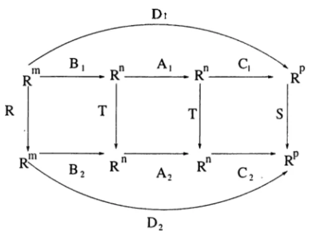
).Many system properties remain unchanged under coordinate transformations in the states, inputs, and outputs.
D e fin itio n 2 .4 .1 . Two LTI systems Si := {Ai, D\) and S
2
:= {A2·, B2 1C2, D2) are called eq u ivalen t if there exist nonsingular matrices T €G such that
A2 = T A f.r -\ B2 = T BxR - \ C2 =■· SCxT - \ D2 = SDxR~\
The systems S i and S
2
ai’e thus equivalent if one can be obtained from the other by nonsingular coordinate transformations in the state space R'^, the input space R ”*, and the output space R ''. Interpreting the matrices as maps, we have the commutative diagram of Figure2.1
for equivalence.Di
2.4
Transformation of Linear Systems
Figure
2
.1
: Equivalence of linear systemsSince A\ and A2 are related by a similarity transformation, the eigenvalues
and their multiplicities remain unchanged under system equivalence. Reach ability is also preserved under equivalence as expected. Given the equivalent systems Si and S
2
, Si is completely reachable if and only ifTi2 is completelyreachable. To see this, note that
B2 A2B2 ... / i r
'^2
(Hag {jR, i?} = 7' B, A ,B , ... A\-^BSince R and T are nonsingular, the result follows by Corollary (2.3.1).
2.5
Separation of the Reachable Part
If a LTI system is not reachable, it is jDossible to identify a maximal “part” of the system which is reachable. The fact that Rq is an ^4-invariant subspace of R " allows one to do this.
D e fin itio n 2.5.1. Given any A € a subspace S Ç R " is said to be A -invariant if Ax € S for all x e S.
E x a m p le 2.5.1. The subspaces {0 } and R " are clearly /l-invariant for any matrix A. If A has all its eigenvalues distinct and real, then the span of any collection of the corresponding eigenvectors is an A-invariant subspace of R ” . Given A e R ” , there is a one-dimensional A-invariant subspace of R ” if and only if A has a real eigenvalue.
Fact 2.5.1. The reachable subspace Rq is the smallest A-invariant subspace containing Im B o / R " .
Proof. Let X € Ro so that x = a.’o + a;i + ... + .r„_i, where Xi € AGm B for i = 0, l,..n — 1. Now Axi € {A^'^^ImB) Ç Rq for i = 0 ,l ,..n — 2 and Axn-i € {A^Im B) Ç 7?-o, where the last inclusion is by Cayle.y-Hamilton the orem. Hence Rq is a A-invariant subspace containing Im B. Any A-invariant
subspace containing Im B in R " should contain A^ImB for i =
0
,1
, . .?r —1
. Therefore, R q is the smallest A-invariant subspace containing Im B. □Let the columns of a matrix Rq be a basis for Rq and let a matrix Ri be such that T := [i?o -f^i] is nonsingular. Since Rqis /l-invariant containing Im B,
there exist matrices /l i , ^
2
, Az and B\ such that Ai A20
/I3
A\Rq — [i?o ^1
] We thus have , B = [R o R i] B, 0 T~^AT = A\^2
, T~^B = ’ B , '0
A3
0
(2.15) Note that dimRo = rank = rank B A B ... A^-^B B, AiBi ... A r^ B i 0 0 0 = rank ^ = rank B A B ... A^-^B Bi AiB i ... A ^^B i Bi AiBi ... A^^-^Bi By Cayley-Hamilton Theorem, this is equal to ra72kwhere ni := siztA\. We have thus shown: 1/ dm iR o = ni < n, then theix exists a nonsingular matrix T such that (2.15) holds fo r some matri ces Aj·, i = 1,2,3 and B\ such that s iz e A i = iii and (Ai,Bi) is a I'eachable pair. The particular form (2.15) attained by system equivalence is called the ■reachable normal form.
An alternative criterion for reachability is as follows.
Corollary 2.5.1. The system (2.1) is (completely) reachable if and only if
rank s i - A B = n,
V.S e c.
Proof. [Only If] Suppose rank s I - A B ^ n, for some s G C , then there exists a nonzero q ^ C ’^such that q '{sl — A) = 0, q'B =
0
. This givesSince
9
0, there exists ci nonzero vector in the left null space of the reacha bility matrix. By Corollary (2..3.1), i A , B ) is not reachable.[If] If { A , B ) is not reachable, there exists a nonsingular T G such that (2.15) holds. Now, for s G (t{Az)·, we have d e t(s l — As) = 0 and hence
rank si — Ai -A-> Bi
0 si - A 3 0
< n then, rankT
-1
( s I - A ) T Bwhich implies that rank s i - A B < n.
< n (2.16)
□
We close this chapter by the following definition, the terminology being explained in Section (3.3).
Definition 2.5.2. The pair (A^B) is called stabilizable if either ( A , B ) is reachable or cr(A3) C C _, inhere A3 is defined by the reachable normal form (2.15).
Corollary 2.5.2. (A,R) is stabilizable if and only if
•'ank s i - A B = n, Vs G Co+. (2.17)
Proof. [If] If (A^B) is not stabilizable, there exists T G as in (2.15), where [A\.,B\) reachable and cr(A
3
) (f. C _ . Hence there exists s G Cq+ ncr(A3
) such that d e t{s l — A3
) = 0 so that (2.16) holds and rankfor this s G Co+ n cr(A
3
).s i - A B < n
[O n ly If] If rank A - A B < n for some s G Cq+, then
rank
s i — A\ —A2 B\
0 s7 - A3 0
< n = rank T- 1 { s I - A ) T B < n.
Let 0 ^ G C " be such that q' — <![ <l2 and
(A (/2
s i — A\ — A2 I3i
0
s i - A30
= 0. (2.18)
By (2.18), q [{sl — Ai) = 0 , q[Bi = 0 so that qi = 0 by reachability of {A i,B i). Hence, again by (2.18), q'^isl —
2
I3
) = 0 for q27
^ 0. Therefore,s G <
7
(^43
) n Cq+. D2.6
Notes and References
The definition of state is due to Belman et al. [
1
], [2]. The theorem for the existence and uniqueness of the solution to (2.1) can be found in [3]. The invariance property (2.4) of (2.1) is explained in detail in Callier and Desoer [4]. The books [5], [6
], [7] can be consulted for further background on stability of systems. The concept of reachability and controllability is introduced by Kcilman [8
] in the context of optimal control. The idea of the separation of the reachable part is due to Kalman [9], [10]. The criterian for reachability in Corollary (2.5.1) is known as Hautus Belevich Popov (HBP) test because original sources include [11
], [12
] and [13]. More fundamental facts of linear algebra used such as Cayley Hamilton theorem and their proofs can be found in [14].Chapter 3
STATE FEEDBACK
A primary objective of control theory is the relocation of the system eigen values in order to achieve desired characteristics such as stability, satisfactory transient response. We assume in this chapter thcit all state variables are avail able for control purposes and show that if system is completely reachable, then any desired characteristic polynomial can be obtained by state feedback.
Consider the state equation in (
2
.1
),x{t) = Ax{ t ) -f t > 0. (3.1)
If the input is a linear constant function of the states, then we can write
u(t) = Fx{ t ) , F e (3.2)
The two equations (3.1) and (3.2) lead to a closed-loop unforced system
x{t) = i A + BF ) x i t ) (3.3)
driven only by the initial state .Tq = .t(0) as shown in Figure 3.1.
3.1
Reachability and Feedback
In this section, it will be shown that exponential stability of the closed loop system with arbitrarily large decay rate can be achieved by state feedback if and only if (3.1) is reachable.
We first note the following properties of the induced matrix norm.
Fact 3.1.1. For every A € o-{A), || A ||:= >| A | .
Proof. Let A be an eigenvalue of A and xi be a corresponding eigenvector. Then, II Axi || = | A ||| xi || so that =| A |. It follows that
II ^-^-ll , I
- I A I ·
□
Proof. Let xi be a corresponding eigenvector of A G cr(A). By the series expansion of the exponential matrix function
e^^xi = xi + A xit + ...+
nl + ...
, X^xif’
—
3;i + Xx\t + .... H
---j---h ···
nl
(3.4)By (3.4), is an eigenvalue of The result follows using Fact (.3.1.1). □
T h e o r e m 3 .1 .1 . The pair (A^B) is reachable if and only if^ ^ > 0, 3F.y € R ”^^" and My >
0
such thate^A+BFAt II< Vi >
0
. (3.5)Proof. [If] Suppose (T , B) is not reachable. Let T € be nonsingular putting {A, B) into reachable normal form as in (2.15). For any F € R '"^ ",
T~AA + B F )T =
^2
’ Bi ' r 1 + F, F20
As0
where F T — F\ F2 . Then T - \ A + B F ) T ^ Ai + BiFi A2F B2F2 0 /1,3 Let A =Ai
+B\F\ A2
+B2F2
0
/I3
By Fact (3.1.2), || eSA+BF)t | j > g f l e { , \ 3 } < ^ where A 3 G
cr(Az).
Suppose nowthat V
7
>0
, there exist Fly and AFy > 0 such that (3.5) holds. Choosing7
> —i?e{A3
}, we haveMye"^‘
>11
e^A+BFAt ||> gHe{A3}<_It follows that
]\L· > (3.6)
Since i?e{A
3
} +7
>0
, (3.6) fails for large t. Hence, if {A, B) is not reachable, then (3.5) is not satisfied for .some7
> 0.[O n ly if] Let
■ = f
-A e u / „-A 's
where is as defined in Lemma (2.3.1) and F ;= —B'Ws~^. Since { A, B) is reachable, by Lemma (2.3.1), We ^ exists. Consider the candidate Lyapunov function V(x) ;= x'WeX for X = (A-\- B F )'x. We have
= 2 x 'e -‘''B B 't-*''A 'xd T + 2x'W ,F'B'x. Hence,
l/(.r) = - r A II B'e-^'^x II dr - 2x'BB'x. (3.7) J
0
cL'i"By (3.7), V{x) < 0. U.sing Lyapunov Theorem, there exists M > 0 such that
II ¿A+BF)'t II ^11 ¿A ^B F)t | | < > g .
Note that, using Corollary (2.3.1) it can easily be shown that, {A^B) is reach able if and only if (/I-I-
7
/ , 5 ) is reachable. Hence, given any7
> 0, there existE,, such that II FA+^^+BF^)t II< M^. So, II ||< Vf > 0. Then
F^ = -B 'W -}^ , (3.8)
where
Wr^ := Jo
The state feedback F^ of (3.8) achieves the desired decay rate in the closed
The expression (3.8) for the state feedback shows that a small amplitude closed loop state and/or a large decay rate, can be achieved at the expense of allowing large magnitudes in the entries of the state feedback, i.e., at the expense of a “high-gain” state feedback.
3.2
Eigenvalue Assignment
If [A^B) is reachable, not only can one achieve an arbitrary decay rate for the closed loop system of Figure 3.1, but can also assign the spectrum of the closed loop system at any given n-points in the complex plane, the only restriction arising due to the fact that the state feedback F is a real matrix. In this section, we first show that, using state feedback, a reachable system can be nicicle reachable from a single input, usually any of the m input components with nonzero effect on the state. The eigenvalue assignment result for single input systems is then used to construct a state feedback achieving the desired spectrum for the original multi-input .system.
L e m m a
3
.2
.1
. Consider (3.1). I f { A , B ) is reachable, then for some b = Bv ^0
, there exist Ui,U2,...tin-i such that the vectorsxi := b = Bv X2 := Ax I + Bui
(3.9)
Xfi .— AXji—{ -f* BUji—i
are linearly independent.
Proof. The proof uses induction on n. For n =
1
, Xi = b ^ 0 and the statement is true. Suppose that are linearly independent. We show that there exists Uk such that xi, ...Xk, Xk+i are linearly independent for k < n. Suppose thcit such Uk does not exist. So0:^+1
= Axk + Buk is in spfm{.ri, ....ca,.}. Let L span{xi, . . . X k } · Then Axk + Buk € T, 'iuk- By setting u = 0, Axk € L.It follows that Buk G L. Hence L is an H-invariant subspace containing ImB. Therefore T 3 by Fact (2.5.1). This implies that k = n. □ L e m m a 3 .2 .2 . I f { A , B ) is reachable and b = Bv ^ 0, then there exists F such that [A + BF., b) is reachable.
Proof. By Lemma (3.2.1), there exist Ui, ..u„_i such that .'Cj, ...,x „ of (3.9) are linearly independent. Let F be chosen such that P'xk = Uk for A; = l,..n —
1
. Then(A + BF) xk = Axk + Buk - Xk+i, k = 1,2..??. -
1
. So, Xk+i = (A + BF)^b, k =1
,2
..?? —1
. Thereforerank = ??.
□
b {A + BF) b ... (A + B F ^ -^ b Hence [A + BF,b) is reachable.
T h e o r e m 3 .2 .1 . The following are equivalent. (i) (A,B) is reachable.
( i i ) For every set F ;= {71,...7,1} C C which is symmetric with respect to the real axis, there exists F such that cr(A + B F ) — F.
Proof, (ii) (i) Suppose that (A ,B ) is not reachable, and let T G put [ A, B) into reachable normal form (2.15). Then
<t(A + B F ) = a(T~HA + BF ) T) = a
’ Ai a/
+
' BiFr B2F2
where F T = Fi F2 . It follows that / a(A + B F ) — a L A\ + B\F\ A-2 + B2F2 0 A3 \ J/ = <r{Ai + BiFi)Ua{A: i ). 3.10)
By (3.10), the eigenvalues of A3 are in a{ A + BF) . So a{ A + B F ) can not be
an arbitrary set.
(i) (ii) If i A , B ) is reachable, then by Lemma (3.2.2), there exists Fi such that {A + BF\., Bv) is reachable for some nonzero Bv. Let A := A + BF\ and b Bv. Note that there exists a transformation matrix T putting (A ,
6
) into control canonical form, i.e., T is such that0 1 0 0
0
0 0 1 00
T A T - i = , tU ■ ^0 ^^1 ^n—11
(.3.11)where d;’s are determined from
d ct(sl — A) — s” -f" ctn—
1
^” "b ... "t" iiii· "b 0,0·Given any V - {
71
, ...,7
„ } G C , let ( s -7
i ) ( s ~72
) . . . ( s -7
„) = : s" + a„_is'^ ^ + ... + Q>lS + CtO) F2^0
~ ^n—1
1
, and F2 := F2T. IfF := F i F VF2, then the spectrum of the closed loop system is
a(A
+BiFi
+VF
2)) = a{T{A
+B{Fr
+vF2))T~^) = a{TAT-^
+ T6A)·By (3.11), a { A ^ B F ) = a 1 0 0 1 0 = a (Xq
^'1
0 1 0 0 - a „ _ i+ a„ - a-o
a„_i - a„_i
1 0
y Cl Q Q>\ ^n —
1
= {Ti.--.Tn} = r.
□
The state feedback F constructed by the algebraic method in Theorem (3.2.1) achieves the decay rate m a x ,{—i? e {
7
i } } for the closed loop system. Similar to the stiite feedback of Theorem (3.1.1), this feedback matri.x also has entries of large magnitude if it achieves a large decay rate since ao ==7
i..-7
n appears in its expression.3.3 Stabilizability
If (A, B) is not reachable, then neither eigenvalue assignment nor exponential stability with arbitrary decay rate is possible in the closed loop system. We show in this section that it is still possible to achieve exponential stability with decay rate being determined by the eigenvalues of the “unreachable part” of {A^B) provided [ A , B ) is stabilizable.
I )
T h e o r e m 3 .3 .1 . There exists a state feedback F G such that cr{A + B F ) C C _ if and only if (^4, B ) is stabilizable.
Proof, [if] Suppose that {A, B) is stabilizable. If (/1, B) is reachable, the result follows by Theorem (3.2.1) on letting T be any symmetric subset of C _ . If [A.,B) is not reachable, then in the reiichable normal form, A-s has all its eigenvalues in C _ . Note that for any T’,
a { A F B F ) = a { r - \ A F B F ) T ) = a A\ /I
2
V
0 A\ + B\F\ A2 + B1F2 \0
A3 / + B, 0 Fi0
where F := F2 —<^(^1
+ U cr{As)^ (3.13) T~^. Since (y4i,i?i) is reachable, there exists F\ such that <7
(/li + BiP\) C C _ . Hence, by (3.13), cr(/l + BP') C C _ .[O n ly If] Suppose that for some F , one has a{A-\-BF) C C _ . Then by (3.13),
«^(As) c C _ . □
By Theorem (3.3.1), the eigenvalues of A^ can not be shifted by any state feedback. For this reason, the matrix A^ of the reachable normal form is sometimes referred to as the “unreachable part” of ( /1 ,5 ) . Also note that all the eigenvalues of A\ of the reachable normal form can be assigned arbitrarily.
3.4
Notes and References
For Lyapunov theorem and its proof, the book [
6
] can be referred to. As reported by Kailath [15], Bertram perhaps was the first one who realized in1959 that if the system was controllable, the desired characteristic polynomial could be obtained by state variable feedback [15]. In 1962, Rosenbrock [16] discussed this problem but a complete statement and result was not given. Eigenvalue assignment problem and complete solution was first published by Rissanen [17], in a similar way, Popov [18] also obtained the same result for the multivariable systems. Lemma (3.2.1) and (3.2.2) in Section (3.2) are due to Heymann [19] and Wonharn and Morse [20]. The control canonical form for a. single input system is first published by Popov [
21
]. A more detailed discussion of stabilizability can be found in [22
].Chapter 4
OBSERVABILITY A N D
OBSERVERS
When the states are not available for measurements or when engagement of all the components of the states for feedback is not desirable, the simplest approach to achieving the control objectives would be to reconstruct the states from available mesurements, the outputs, and then apply the known state feedbcick technicpies. The most direct means of reconstructing the states is to design cui observer. Whether the states can be reconstructed at all is an issue that must first be studied. This gives rise to the concept of observability. In this chapter, we discuss the concept of observability and the design of dynamic and functional observers for a LTI system.
4.1
Observability
Consider the LTI system (2.1) with (p{t;to,Xo,ui·)) denoting the value at time t > 0 of the trajectory resulting by the initial state xq at to and by the appli cation of input ■«(.) in [^
0
?^]· Also let r]{t,(p{t;to.,XoiU{.)), u{.)) be the value of the output at time i >0
resulting from application of the input ■u{.) in starting with the initial state Xq-D e fin itio n 4 .1 .1 . A state Xq G R ” is said to be u n o b s e rv a b le in [^o, ^i] if
= 0, Vi € [io.il], io < <i (4.1)
i.e., when no input is applied, the state xq gives rise to zero output at all times in [to,^i]·
Note that if xq is unobservable in then its effect on the out put is indistinguishable from that of the zero initial state x{to) --
0
since r/(t, (^(i; ¿o, 0, 0), 0) = 0. In what follows, we show that, as a consequence of time-invariance of (2
.1
), the interval of unoKservability is imniciterial.T h e o r e m 4 .1 .1 . The following are equivalent:
(i) A state xo G R '‘ is unobservable in [io^i] fov some to < t\ . (<>) e n?=o
KtrCA'.
(iii) .To is unobservable in [i,>s] for any t < s.
Proof. It is obvious that (iii) (i). (i) (ii): If .tq is unobservable in [io, ^i], then by (4.1) and (2..3),
The last equality evaluated at t — to gives Cxq =
0
. Taking the derivative of both sides of this equality successively and evaluating at t — to·, we obtainCA^Xo =
0
, i —0
,1
, n —1
.Hence, xo €
0
^=0
^ K erC A \(ii) ^ (iii) If (ii) holds, then by Cayley-Hamilton theorem, CA''Xo =
0
for all i > 0. It follows that for any t < s.,f ] ( t , ( p i T - , s , X o , u { . ) ) , 0 ) = = 0, Vr e [ t , s ] ,
by the series expansion of the matrix exponential. Thus, xo is unobservable in
[t,s]. □
Let us define the unobservable subspace of (2.1) by
T]o := {:i‘o ^ R " : Xo is unobservable in [
0
,i] for some i >0
}.By Theorem (4.1.1),
n
—1
7
/0
= f ] K e r C A \i= 0
so that
7/0
is a subspace of R ” .F act 4 .1 .1 . The unobservable subspace 7/0 is the largest A-invariant subspace
contained in K e r C o / R " .
Proof. By Cayley-Hamilton theorem, 7/0 is H-invariant. Moreover, it is the
largest H-invariant subspace contained in K e r C . To see this, note that any other such subspace 7/ satisfies 7/ C K e r C and, by H-invariance, it also satisfies
A^Tj C K e r C which implies 7/ C K e r C A ’^ for i = 0, . . . , 77 — 1 . hlence, 7/ C 7/0. □
Suppose T]o ^ {0 }. Let the columns of a matrix 7Vo be a basis for r/o and let a matrix Ni be such that T := [A^o -^i] is nonsingular. Since span Nq is .4-invariant in K e r C , for some matrices Ai, i -- 1,2,3 and C\, the following equalities hold:
AT = T Ai A2
0 A3
,
CT =
0Cl
(4.2)where si zeAz = dim.riQ. Since span No is the largest A-invariant subspace in K e r C , it also follows that
n
—1
na-l
dim Pi / ’fe rC iA g = P KerCiA^ = siztA:^ = n — dimrjo·
i= 0 t=0
Alternatively, note that
n—dim rjo — rank
c
0
Cl Cl C A T -- rank0
Cl A3 = rank Cl A30
• C A ” - ! /0
C i A r ' _ C i A r ' _ By Cayley-Hamilton theorem, C Cl rank C A — rank Cl A3
C A ” - ! _ C iA ”^-i _ so that dim(^”¿0
^ C'l A3
= size A3 = n — dim rjo.D e fin itio n 4 .1 .2 . We call the system (2.1) or the pair (C^A) o b s e r v a b le if Vo = {0 } ■ The system (2.1) or the pair (
6
’, A ) is called d e te c ta b le if a (A i) C C _ , where A\ is as defined by (f.2).Note that tjo = {()} if and only if rank C CA
t ,\n-i
C A = n.We have shown above that if a system (2.1) is not observable, then it is equivalent to a system
(
0
ClAi A2
0 A3
(4.3)
where (C i, A
3
) is observable and si z eAi = dimîjQ. The sytem (4.3) is referred to cVS the observable normal form.C o r o lla r y 4 .1 .1 . The pair (C, A) is observable if and only if
rank s i - A C
= for all s
6
C.Proof. [O n ly If] If rank
s i - A C
< n, for some
5
€ C , then there exists a nonzero q E C"' such that q'{sl — A') = 0, q 'C =0
. This givesC A 'C ... A d "-i)C ' = 0. Since q' ^ 0, rank C C A r /in-l C A < n.
[If] If (C*, A ) is not observable, there exists a nonsingular T E such that
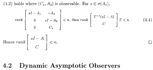
(4.2) holds where {C\^Az) is observable. For s € (7(/li), rank s I - A i —Ao 0 si - A3 < n, then rank r ~ ^ ( s l - A ) 0 ^7 c T < n. (4.4) Hence rank s i - A C
< n.
□
4.2
Dynamic Asymptotic Observers
Except in some trivial cases where the matrix C has full row rank, any re construction of the state a;(
0
) from the measurements t/(i), t € [0
,ii] in the LTI system (2
.1
) necessitates dynamic processing. An asymptotic observer is a LTI system, the output of which asymptotically tracks the states of (2
.1
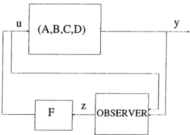
). It is driven by the available system inputs and outputs. A block diagram of the asymptotic state reconstruction process considered in this section is given in Figure 4.1.Figure 4.1: Open loop system state reconstruction
Consider a LTI system
where J G G and L G R"''^™. The system (4.5) is a can didate observer for (2.1) and the vector z{t) is called the observer state. The system (4.5) is called a full-state observer if for all initial states .to,^o G R ” , and for every input u{t),
lim II x(t) - z{t)
11
=0
,1—+00
where x(t) and z{t) are the solutions of (
2
.1
) and (4.5), respectively. Let us define the error vector bye{t) = z[t) — .'c(t), t > 0.
The error obeys the equation
e(t) = J z { t ) K y { t ) L u { t ) — Ax{t) — Bu{t) = Jz{t) + KC x ( t ) + KDuf t ) — Ax{t) — Bu(t)
= (A - KC) e { t ) + {3 - A + KC) z { t ) + {L - B + KD) u( t) . Setting J = A - K C \ L = B - K D , (4.6) (4.7)
the error equation simplifies to e{t) = Je{t). If cr(,/) C C _ , then limt_oo || e{t) 11= 0 for all eo = zq — Xq. Any observer satisfying the special choice (4.6) is called a L u e n b e r g e r o b se rv e r. It is clear that (4.5) is a Luenberger observer if and only if there exists K G R "^ ”^ such that a [A — K C ) C C _ . The order of the Luenberger observer is thus equal to the order of the system it observes. The decay rate of the Luenberger observer, when it exists, is defined as the decay rate of the (exponentially stable) error system e(t) = (A — liC )e (t ). The crucial matrix K is called an output injection matrix for the system (
2
.1
).We now examine the conditions under which a Luenberger observer exists. T h e o r e m 4 .2 .1 . The following are equivalent:
(i) {C^A) is observable.
(ii) For every
7
> 0, there exists a Luenberger observer for (2.1) achieving a decay rate7
for the error system.(iii) For all symmetric family o f n complex numbers A, there exists K such that a{A - K C ) = A.
Proof. Note that (C, A) is observable if and only if (A ', C ) is reachable, as C rank CA < /1 7 1 - 1 C A — rank C A 'C ( A T ' ^ C
Hence, the result follows from Theorem (3.1.1) and Theorem (
3
.2
.1
) upon re placing A, B, and F by A', C , and —K, respectively. □Thus, observability of (2.1) is a necessary and sufficient condition for the existence of a Luenberger observer of arbitrarily large decay rate. Note that the same comment in Chapter 3 concerning large decay rate also applies here, i.e., a large decay rate in the observer is achieved by high gain output injection. If the decay rate is of no particular concern, then an observer exits under weaker condition.
C o r o lla r y
4
.2
.1
. The following are equivalent: (i) (C, A ) is detectable.(ii) There exists a Luenberger observer for (2.1). (iii) There exists K such that cr(A — K C ) C C _ .
Proof. (i)=4* (ii): ( C, A) is detectable if and only if cr(Ai) G C _ , where A\ is in (4.2). Note that a{.J) = a( A - K C ) = a [ t- \ A - K C ) T ) = <7 A: A.
2
-A \ C \0
^3 - /12^1
(4.8) where / { := A'l AAand 7] A
2
, A3
, Cl are as in (4.2). Since (C ijA s ) is ob servable, there exists A2
such that <j(A3
—K2Ci)
C C _ . Hence,cr{J)
C C _and limi_oo || e(i) ||= 0, for all initial states Cq — zq — .Tq. So, there exists a Luenberger observer.
( i i ) => (iii)· If there exists a Luenberger observer, then the error system is asymptotically stable and
a { J ) = a { A - K C )
C C _for some K .
( i i i ) =^ (i): If there exists
K
such thata {A — K C )
C C _ , then using (4.8) <^(411
) C C _ . This implies that{C,A)
is detectable. □4.3
Functional Observers
As cin application of ideas used in obtaining a Luenberger observer, we now consider construction of functional observers whicli find applications in fault diagnosis. See e.g., [2.3].
If not the whole state but the reconstruction of some linear combinations of state components x f t ) € R ” , i =