Non-boltzmann stationary distributions and non-equilibrium relations in active baths

NON-BOLTZMANN STATIONARY

DISTRIBUTIONS AND NON-EQUILIBRIUM

RELATIONS IN ACTIVE BATHS

a thesis submitted to

the graduate school of engineering and science

of bilkent university

in partial fulfillment of the requirements for

the degree of

master of science

in

physics

By

Aykut Argun

September 2016

BOLTZMANN STATIONARY DISTRIBUTIONS AND NON-EQUILIBRIUM RELATIONS IN ACTIVE BATHS

By Aykut Argun September 2016

We certify that we have read this thesis and that in our opinion it is fully adequate, in scope and in quality, as a thesis for the degree of Master of Science.

Giovanni Volpe(Advisor)

G¨okhan Barı¸s Ba˘gcı

Seymur Jahangirov

Approved for the Graduate School of Engineering and Science:

Ezhan Kara¸san

ABSTRACT

NON-BOLTZMANN STATIONARY DISTRIBUTIONS

AND NON-EQUILIBRIUM RELATIONS IN ACTIVE

BATHS

Aykut Argun M.S. in Physics Advisor: Giovanni Volpe

September 2016

Most natural and engineered processes, such as biomolecular reactions, protein folding, and population dynamics, occur far from equilibrium and, therefore, can-not be treated within the framework of classical equilibrium thermodynamics. Here, we experimentally study how some fundamental thermodynamic quantities and relations are affected by the presence of the non-equilibrium fluctuations as-sociated with an active bath. We show, in particular, that, as the confinement of the particle increases, the stationary probability distribution of a Brownian particle confined within a harmonic potential becomes non-Boltzmann, featuring a transition from a Gaussian distribution to a heavy-tailed distribution. Because of this, non-equilibrium relations (e.g. Jarzynski equality, Crooks fluctuation the-orem) cannot be applied. We show that these relations can be restored by using the effective potential associated with the stationary probability distribution. We corroborate our experimental findings with theoretical arguments.

¨

OZET

AKT˙IF BANYOLARDA BOLTZMANN DIS

¸I DURGUN

DA ˘

GILIMLAR VE DENGE DIS

¸I TERMOD˙INAM˙IK

YASALARI

Aykut Argun Fizik, Y¨uksek Lisans Tez Danı¸smanı: Giovanni Volpe

Eyl¨ul 2016

Biyomolek¨uler reaksiyonlar, protein katlanması ya da populasyon dinami˘gi gibi bir¸cok do˘gal ve tasarlanmı¸s proses denge durumundan uzakta cereyan eder, dolayısıyla klasik termodinamik ile modellenemez. Bu ¸calı¸smada, bazı temel termodinamik niceliklerin ve denklemlerin aktif bir banyonun varlı˘gından kay-naklanan denge dı¸sı dalganalanmalardan nasıl etkilendi˘gini deneysel olarak in-celiyoruz. Ozellikle Brown par¸cacı˘¨ gının dar bir alana sıkı¸stırılması, durgun olasılık da˘gılımının Boltzmann dı¸sına ¸cıkmasına ve Boltzmann da˘gılımından a˘gır kuyruklu bir da˘gılıma ge¸ci¸sine sebep olmaktadır. Bu nedenle, denge dı¸sı termod-inamik yasaları (¨orne˘gin, Jarzynski denklemi ya da Crooks dalgalanma teoremi) bu sistemlere uygulanamaz. Bu problemin durgun olasılık da˘gılımını kullanarak elde edilen efektif bir potansiyel kullanılarak d¨uzeltilebilece˘gini g¨osteriyoruz. Bu deneysel bulgularımızı teorik kanıtlar ile destekliyoruz.

Anahtar s¨ozc¨ukler : stokastik termodinamik, denge dı¸sı termodinamik denklemler,

Acknowledgement

This research has been completed during my Master’s studies. Here, I would like to thank to all people who has contributed to my motivation during the last two years.

First of all, I want to highlight the contribution of my family to my research as they have always been supportive about my academic goals. They have not judged a single decision I ever made in my life, some of which I believe looked pretty crazy from their picture. I know how much proud of me you are and I also know that I will overcome any problem in my life no matter how tough it is in order not to dissappoint you. I cannot tell how lucky I am to have you.

In addition to my family, I would like thank my close friends who have always supported me. Abdullah, we have spent 8 years together in Ankara and have shared a lot. I do not even know how to thank you, thanks for all of your support and friendship. In addition, I want to highlight the contributions of Mustafa, it was a pleasure for me to be your translator :) I am sorry to inform Murat that his efforts to distract me from science has not been successful, I am finally here at the last step of my Master. I want to thank Davut, Oguz, Bilal, Enes, Tugrul, Salih, Erion, Yusuf, Selim, Ali and Hakan for their support.

I also want to thank sincerely to all members of Soft Matter Lab. All of this would not have been possible if I have not been in such an amazing research group. Joining this group was one of the best decisions I ever made, not only because of the scientific productivity, but also because we had a wonderful social environment. As a person who have been in the group for over four years, I have witnessed the best of helpfulness and friendship. Also, our group has been quite active in terms of scientific events, we hosted one IONS and two COST action meetings in Ankara. As a Master student, I had the opportunity to participate in 4 COST action meetings and 2 international conferences, which provided me with a lot of experience and a good network. Particularly, I would like to thank Sabareesh and Sathya for helping me with all the experimental protocols that I

vi

learned, Agnese for teaching me how to use Latex and helping us as a lab manager, Elif for taking care of administrative things, Tugba for tips regarding official documents, and Jalpa for providing feedback on my thesis. I also sincerely thank the rest of the group: Masoumeh, Alex, Mehdi, Fatemeh, Mite, Naveed, Geet, Merve, Ehsan, Falko, Serdar, Murad, Bora, Pascal, Yagmur and Muhammeds, thank you so much for all the unforgettable times we had. In addition, I highlight the contribution and support from my department, all of the faculty members and Fatma Gul.

I also want to highlight the contribution and support that I have received from my coauthors. Thanks Ali-Reza for introducing me experimental optics and working principles of light modulators. Thanks Ercag for his help regarding the bacteria production, I have learned a lot from him. I thank sincerely to Baris hoca, who has always supported my studies and appreciated so much that I generally felt overrated. He has been a very close friend with me apart from being a collaborator. Also, I want to thank to Seymur hoca, who participated in my defense as a committee member. It is a pleasure for me to have such a young and yet very bright scientist in my jury.

Finally, I would like to thank to my advisor. Dear Giovanni, I have spent a lot of time thinking a way to express how much I appreaciate your supervision, but I figured out that it is beyond my writing skills. Thanks for coming to Bilkent and contributing to my country...

Contents

1 Introduction 1

2 Introduction to Stochastic Thermodynamics 5

2.1 Thermodynamics in the microscopic world . . . 7

2.1.1 Solution of the Langevin equation and derivation of the Boltzmann distribution in a thermal bath . . . 7

2.1.2 Stochastic energetics . . . 11

2.1.3 Stochastic heat engines . . . 17

2.2 Irreversibility, second law of thermodynamics and the role of fluc-tuations in small systems . . . 19

3 Fluctuation Theorems 22

3.1 Crooks Fluctuation Theorem . . . 24

3.2 Jarzynski equality . . . 32

CONTENTS viii

4 A non-Markovian environment: Active matter 38 5 Equilibrium or non-equilibrium?

Results on experimental investigation of stationary

distribu-tions 42

5.1 Non-Boltzmann stationary distribution in active baths . . . 44

6 Results on experimental investigation of non-equilibrium rela-tions in active baths 51

7 Conclusion 60

A Experimental Methods 74

A.1 Optical trapping and experimental setup . . . 74

A.2 Bacterial sample preparation . . . 75

A.3 Data analysis . . . 76

B Codes 77

B.1 Figure 2.1 - Demonstration of Boltzmann distribution for a con-fined Brownian particle . . . 77

B.2 Example 2.1 - Isochoric heating . . . 78

B.3 Example 2.2 - Isothermal compression . . . 80

B.4 Example 3.1 - Crooks fluctuation theorem in an arbitrary process 81

List of Figures

2.1 Demonstration of Boltzmann distribution for a confined Brownian particle. . . 10

2.2 Illustration of an isochoric process. . . 14

2.3 Illustration of an isothermal process. . . 16

2.4 Experimental realization of a microscopic colloidal heat engine . . 18

3.1 The same forward and backward trajectories under time reversal in a non-equilibrium process. . . 25

3.2 Verification of Crooks fluctuation theorem in an arbitrary process. 30

3.3 Experimental verification of Crooks fluctuation theorem. . . 31

3.4 Illustration of Jarzynski equality in a time-dependent harmonic trap. 35

3.5 Experimental free energy reconstruction using Jarzynski equality . 36

4.1 Mean square displacement (MSD) of active Brownian particles and effective diffusion coefficients. . . 40

LIST OF FIGURES x

5.2 Particle in an active bath. . . 48

6.1 Violation of Crooks fluctuation theorem in an active bath. . . 55

6.2 Recovery of Crooks fluctuation theorem in an active bath using effective potentials. . . 57

6.3 Verification of Jarzynski equality and integral fluctuation theorem in an active bath using effective potential. . . 59

Chapter 1

Introduction

In the 19th century, classical thermodynamics had a major effect on development of industry and automation. A long journey of countless investigations began with an intense study of heat engines, highly stimulated by the development of the transportation sector after the industrial revolution. At the time, it was crucial to use vapor engines with the highest possible efficiency, and therefore, scientist looked for the limits that the nature had set via thermodynamic laws. The first and second laws of thermodynamics, as crucial cornerstones in classical thermodynamics, were discovered in a relatively short time interval [1].

One of the most significant steps forward in classical thermodynamics is the discovery of its relation with information in the mid 20thcentury. Scientists found the thermodynamic limits of information-to-energy conversion and the costs of information erasure. These theories became extremely appealing especially after the computer industry got closer to these limits. For instance, heat dissipation in the processors is one of the biggest problems for hardware developers, which is directly connected to the Landauer’s limit [2]. Landauer himself was a computer scientist but he is also considered to be one of the biggest contributors to the thermodynamics of information processing.

proven to be valid for macroscopic systems, where a system has a gigantic number of components or particles such that there are superabundant degrees of freedom therefore ensemble averaging for a system is reasonable. However, as soon as sci-entists had access to microscopic systems, they immediately realized that some of the fundemantal laws of thermodynamics do not always hold for such small systems. In 1993, for example, scientists observed that the 2nd law of thermody-namics might be violated for small systems at short timescales. Nevertheless, the 2nd _{law was shown to be correct in average [3].}

Within the last two decades, as stochasticity is largely incorporated into modynamics, researchers have shown that not only the average values of ther-modynamic quantities give us information about a system, but also fluctuations around the mean values for stochastic systems store significant amount of infor-mation about an irreversible microscopic process. It has been shown that these fluctuations have to follow certain statistical conditions. Therefore, we can ex-tract equilibrium information from non-equilibrium data via repeating the mea-surement numerous times. These relations, such as Jarzynski equality [4], Crooks fluctuation theorem [5] and the integral fluctuation theorem [6], have been tested on various systems such as RNA stretching [7, 8], mechanical [9, 10] and colloidal [11] experiments. One of the key common point for all of these experiments is the fact that they were all thermalized with a heat reservoir.

Active systems, however; are generally considered to be instrinsically out-of-equilibrium [12, 13]. Whether particles in such active baths can be considered as equilibrium states is yet ambiguous. This ambiguity arises from the fact that the forces acting on a Brownian particle in an active bath are non-Markovian [14]. There have been studies where these systems can be generalized to equi-librium systems with effective temperatures [15, 16]. However, several studies showed that the resulting behaviour of such systems exhibit certain phenomena that are highly unlikely to be observed in a thermal equilibrium system with any possible effective temperature [17, 18]. Thus, it is an open and appealling question whether thermodynamic equilibrium conditions and non-equilibrium re-lations such as Crooks fluctuation theorem (CFT), Jarzynski equality (JE) and the integral fluctuation theorem (IFT) can be employed in an active bath.

In this work, we have analyzed and quantified the active noise associated with an active bath, which we realized experimentally by growing motile bacteria cul-ture (E.coli). We report that when a particle is confined into a potential with large length scales, compared to the correlation length of active noise (i.e. persistence length), the particle’s behaviour follows Boltzmann statistics with an effective temperature; thus, this case can then be treated as equilibrium. However, when we confine the particle into smaller length scales than the persistence length, the particle shows qualitatively different behaviour than the case of equilibrium and its distribution cannot be fitted to Boltzmann statistics with any possible effec-tive temperatures. We conclude that at such scales, it is not possible to treat active bath systems as equilibrium systems.

After this step, we performed for the first time, non-equilibrium work measure-ments for a particle in an active bath. We drived an external optical potential and calculated the thermodynamic work applied to the particle and the heat ex-change between the particle and the active bath. Following from these results, we have shown that in the non-Boltzmann regime, fluctuation theorems are no longer valid. Nevertheless, we report that non-equilibrium relations such as CFT, JE and IFT can be recovered by introducing an effective potential, which is es-timated from the stationary distribution of the particle in the optical trap with imposing Boltzmann distribution.

The rest of this thesis includes five chapters and a conclusion. I will first give a summary on microthermodynamics and stochastic thermodynamics (chapter 2). Then I will give a detailed description of fluctuation theorems with numerical illustrations along with experimental verifications in the literature (chapter 3). I will then introduce the fundamental properties of an active matter system (chap-ter 4). Finally, I will share my results related to the stationary distributions of a particle in an active bath (chapter 5) and non-equilibrium measurements (chapter 6) before the conclusion.

To sum up, in this thesis, I report violations of some cornerstones of classical thermodynamics such as the Boltzmann relation as well as some fundamental fluctuation theorems of thermodynamics in active baths. This outcome arises

from the fact that in an active bath, there is time-correlated (non-Markovian) noise associated with the active bath which we characterize with our experimental data. We also show that these violated relations can still be recovered using effective potentials that would satisfy Boltzmann relation.

Chapter 2

Introduction to Stochastic

Thermodynamics

One of the most fundamental concepts in thermodynamics, and indeed one of the earliest, is reversibility. It was introduced by Sadi Carnote in 1824 within his studies on heat engines, which later led to the 2nd law of thermodynamics [19, 20]. A reversible process occurs when a thermodynamic protocol is applied infinitely slow such that there are no permanent changes in the universe, i.e., one can revert the system to its initial conditions if the reverse protocol is followed. On the other hand, an irreversible process occurs in a finite time and therefore results in heat dissipation in the medium. This is a permanent change because once the heat is dissipated to the heat bath that is in contact with our system, there is no way to collect that heat back without an additional cost of energy. The second law of thermodynamics, which is also described as ‘time’s arrow’ acquired its quantitative form after the concept of entropy was proposed:

dS ≥ 0 (2.1)

where dS denotes the total entropy change in the universe. If one considers the entropy of a system (Ssys) and the entropy of the environment (Senv) separately, S = Ssys+ Senv. Then Eq. (2.1) becomes:

dSsys + dSenv ≥ 0. (2.2)

If we combine the above equation with the 1st _{law (dW = dU + dQ) and the}

definition of free energy (dF = dU − T dSsys) we end up with a different version of the second law [21]:

dW ≥ dF. (2.3)

Eq. (2.3) states that, in any thermodynamic process, the work applied on the system has to be greater than or equal to the change in free energy. Therefore, free energy acts as a lower bound to the amount of work to be applied in a thermodynamic process, or an upper bound to the amount of extracted work when the change in free energy is negative.

The difference between the work done and the change in free energy is called dissipated work [1]:

dWdis= dW − dF ≥ 0 (2.4)

In reality, not only the work we apply during a thermodynamic process, but also the fluctuations of the work applied contain information about the prop-erties of the initial and final equilibrium states, which is going to be discussed in detail in chapter 3. In this chapter, I will give an overview about stochastic thermodynamics and the role of fluctuations on the 2nd law of thermodynamics (Eq. (2.3)).

2.1

Thermodynamics in the microscopic world

In this section, I discuss how fundamental thermodynamic quantities are calcu-lated within the context of stochastic thermodynamics. All the thermodynamic relations and fluctuation theorems are discussed in this context. Also, the math-ematical notation that is introduced in section will be consistently used in the rest of this thesis.

A micron-sized particle immersed in a liquid, which is called a Brownian parti-cle, is assumed to be in contact with a thermal bath if the liquid has well-defined and constant temperature. Because of the random collisions between the particle and liquid molecules, this particle is subject to a stochastic force named thermal noise. Therefore, the resulting equation of motion reads [22, 23]:

md 2_x dt2 =−γ dx dt + √ 2kBT γWx(t) (2.5)

where γ represents the viscosity of the medium, kB is the Boltzmann constant, T

is the temperature of the liquid, and Wx(t) represents the Gaussian white noise

associated with the stochasticity of the system. Without losing any generality, we will mostly be dealing with one dimension only (the x−axis). All of the equations we are going to deal with are also valid for y− and z− axes, but the equations are separable as the thermal noise components are independent.

2.1.1

Solution of the Langevin equation and derivation of

the Boltzmann distribution in a thermal bath

Consider a Brownian particle confined within a potential well U (x). In this case, the particle’s equation of motion will have the form:

md 2_x dt2 =−γ dx dt − dU (x) dx + √ 2kBT γWx(t) (2.6)

For most micron-sized Brownian particles immersed in watery solutions, as the viscous forces are dominant over the inertial forces, the inertial term (m¨x)

can be neglected [24]. Therefore, we can make use of the overdamped version of Eq. (2.6): dx dt =− 1 γ dU (x) dx + √ 2kBT /γWx(t) (2.7)

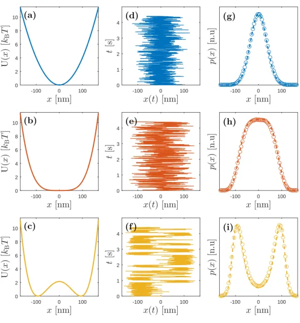
Although there are significant challenges to numerically solve stochastic dif-ferential equations, particularly with the infinite variance of white noise, it is possible to solve Eq. (2.7) with finite difference methods [25, 26, 27]. By numer-ically simulating Eq. (2.7), I obtained trajectories for various potentials, which are shown in Fig. 2.1(d), Fig. 2.1(e) and Fig. 2.1(f).

It is also possible to solve Eq. (2.7) analytically by using the Fokker-Planck equation [28]: ∂tP (x, t) = 1 γ∂x ( dU (x) dx P (x, t) ) + kBT γ ∂ 2 xP (x, t) (2.8)

P (x, t) denotes the probability density function of the particle as a function of x

and t. We are looking for an equilibrium distribution after the particle spends enough time to thermalize in the potential for which ∂tP (x, t) = 0, i.e., when P

is a function of x only. When this is the case, the left handside of the Eq. (2.8) vanishes and we obtain:

−∂x ( dU (x) dx Peq(x) ) = kBT ∂x2Peq(x) −dU (x) dx Peq(x) = kBT ∂xPeq(x) + C Peq(x) = C exp ( −U (x) kBT ) (2.9)

where C = _Z1 = (∫ exp (

−U (x) kBT

)

)−1 can be found via normalization with the partition function Z = ∫ exp

(

−U (x) kBT

)

. Therefore, this proves that a Brownian particle subject to thermal noise will reach the Boltzmann distribution when it is confined in any stable potential well. This relation is also verified numerically from the distribution of the data obtained by simulating Eq. (2.7) for various potentials and shown in Fig. 2.1(g), Fig. 2.1(h) and Fig. 2.1(i).

Satisfying Boltzmann distribution, however, is not enough for a system to be considered in equilibrium. The system should not have any probability current, therefore the probability of forward and backward transitions for any two states that are accesible should be the same. Assuming we have two states S1 and S2

with energies U1 and U2, the transition rates in both directions should be the

same: p1(t)p [S2(t + ∆t)| S1(t)] = p2(t)p [S1(t + ∆t)| S2(t)] exp ( −U1 kBT ) p [S2(t + ∆t)| S1(t)] = exp ( −U2 kBT ) p [S1(t + ∆t)| S2(t)] (2.10)

this condition is named detailed balance [1] and requires equal rate of transitions between the two states. A consequence of this relation is the ratio of conditional transition probabilities between two equilibrium states:

p [S2(t + ∆t)| S1(t)] p [S1(t + ∆t)| S2(t)] = exp ( −(U2− U1) kBT ) (2.11)

We will make use of this relation in the next chapter when I will give the derivation of Crooks fluctuation theorem.

x [nm] -100 0 100 U (x ) [kB T ] 0 2 4 6 8 10 (a) x [nm] -100 0 100 U (x ) [kB T ] 0 2 4 6 8 10 (b) x [nm] -100 0 100 U (x ) [kB T ] 0 2 4 6 8 10 (c) x(t) [nm] -100 0 100 t [s ] 0 1 2 3 4 (d) x(t) [nm] -100 0 100 t [s ] 0 1 2 3 4 (e) x(t) [nm] -100 0 100 t [s ] 0 1 2 3 4 (f ) x [nm] -100 0 100 p( x ) [n .u ] (g) x [nm] -100 0 100 p( x ) [n .u ] (h) x [nm] -100 0 100 p( x ) [n .u ] (i)

Figure 2.1: Demonstration of Boltzmann distribution for a confined

Brownian particle. (a),(b) and (c): Various confining potentials such as a

harmonic potential (a), a quartic potential (b), and a bistable potential (c) are shown. (d), (e) and (f ): Corresponding sample trajectories of a colloidal particle with radius R = 1 µm under the confining potentials shown in (a), (b), and (c), respectively. Trajectories are obtained by numerically solving Eq. (2.7). Matlab code is provided in the appendix B. (g), (h) and (i): Resulting numerical prob-ability distributions (circles) of the particles obtained from trajectories, which are in perfect agreement with the theoretical probability ditributions given by Eq. (2.9)

2.1.2

Stochastic energetics

In classical thermodynamics, we do not apply work on a system unless we ex-ternally control a confinement parameter of the system [1]. For example, for an ideal gas, we do not apply work unless we change its volume. During such a thermodynamic process, there is only heat exchange between the bath and the system.

For microscopic systems, however, how to quantify the heat exchange and work applied on a Brownian particle in a stochastic system has only recently been sorted out. Sekimoto integrated the principles of thermodynamics with stochastic systems which are driven by Langevin equations [29, 30]. He also discussed the first law of thermodynamics at microscopic scales within the context of stochastic energetics.

Let’s consider a Brownian particle confined in a potential U (x), which is only a function of the position of the particle and kept constant over time. As we do not change the confinement parameter of the system, we do not apply any work on the particle. Due to fluctuations, however, there is always heat exchange between the particle and the bath. Since there is no work applied, all the change in the particle’s potential energy comes from the surrounding heat bath:

dU = dQ

Therefore, the heat transferred from the thermal bath to the particle can be written as:

dQ = ∂U (x)

∂x dx (2.12)

Unlike macroscopic systems, heat exchange between the particles and heat bath cannot be isolated for Brownian particles as they are immersed in liquid solutions and they constantly collide with surrounding molecules. Thus, it is not trivial to operate an adiabatic process in such systems [31].

a control parameter λ(t), which is an arbitrary function of time. Then, we are also going to apply work on the particle through the variation of the potential:

U = U (x, λ(t)) dU = ∂U (x, λ(t)) ∂x dx | {z } dQ +∂U (x, λ(t)) ∂λ dλ (2.13)

The first law of thermodynamics states [30]:

dU = dQ + dW (2.14)

Combining Eq. (2.14) and Eq. (2.13) yields:

dW = ∂U (x, λ(t))

∂λ dλ (2.15)

Therefore, we apply work on a Brownian particle when we change the potential parameters. The reversibility condition for such a process will be discussed soon.

Example 2.1: Isochoric heating

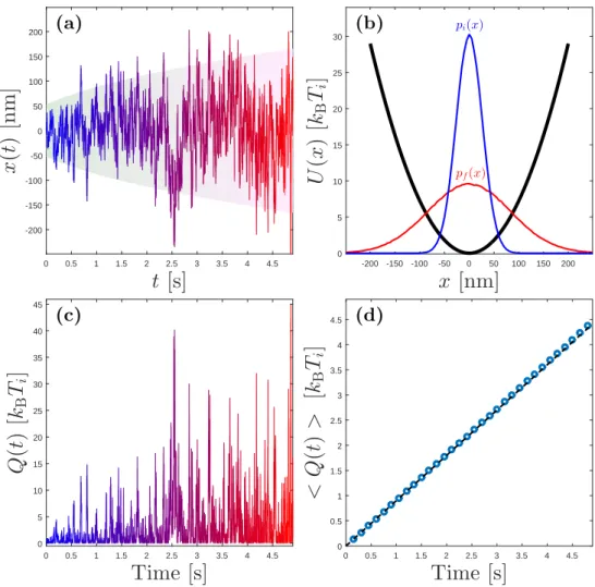
The thermodynamic process involving the heating of the medium sur-rounding a particle held in a harmonic trap can be illustrated by the fol-lowing example. Consider a Brownian particle with radius (R = 1 µm) is immersed in a liquid and the temperature of the medium is raised from

Ti = 50 K to Tf = 500 K over 5 seconds while the particle is confined in

a constant harmonic potential:

U (x) = 1

2kx

2

Since the potential parameters are kept constant, we do not apply any work on the system but we only heat the surrounding bath; this is an illus-tration of an isochoring heating in stochastic thermodynamics. Therefore, the Langevin equation that will govern the non-equilibirum dynamics for this specific process will take the form:

dx dt =− 1 γkx + √ 2kBT (t)/γWx(t) (2.16)

This equation is simulated and a sample resulting trajectory is shown in Fig. 2.2(a). The average potential energy of the Brownian particle in this harmonic trap can easily be calculated and shown to be in agreement with the equipartition theorem [1]:

⟨U(x)⟩ =

∫

p(x)U (x)dx = kBT

2 (2.17)

Since for our example Tf = 10Ti, the final probability distribution of the

particle will be expanded (shown in Fig. 2.2(b)) and change in its poten-tial energy will be ⟨∆U(x)⟩ = kB(Tf−Ti)

2 =

9kBTi

2 . This average is verified

by my numerical example and shown in Fig. 2.2(d), but it is important to note here that the fluctuations are very important in stochastic systems as the heat exchange in a single realization has a completely different profile than the average (Fig. 2.2(c)).

t

[s]

x

(t

)

[n

m

]

x

[nm]

U

(x

)

[k

T

]

Time [s]

Q

(t

)

[k

T

]

Time [s]

<

Q

(t

)

>

[k

T

]

Figure 2.2: Illustration of an isochoric process. (a): Sample trajectory of a Brownian particle in a harmonic trap which undergoes an isochoric heating as described in Example 2.1. The particle’s trajectory is shown and color-coded with the temperature as a function of time. The red color represents hot and the blue represents cold. The background shading represents particle’s standard deviation in the trap as a function time. (b): Constant potential energy is

shown. Also, the particle’s initial and final position distributions within this trap are shown. (c): Heat exchange between the bath the particle. Note that the fluctuations play a very important role and they are much bigger than the average heat transfer, shown in (d). (d): The average heat transfer (circles) and the change in particle’s average potential energy (dashed line) are shown. Since this process is operated during a long enough time (5 s), this two average quantities match. The simulation codes are provided in appendix B.

Example 2.2: Isothermal compression

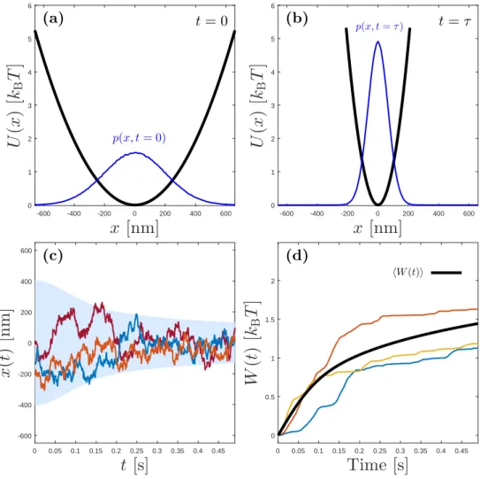
In this numerical example, we will explore how work is applied on a Brownian particle during a non-equilibrium process. Unlike Example 2.1, here we keep the temperature constant, but change the stifness of the confining trap from ki = 1 pN/µm to kf = 10ki = 10 pN/µm. This

protocol is illustrated in Fig. 2.3(a). During such a process, since the temperature is kept constant, the average potential energy of the particle will not change due to equipartition theorem (Eq. (2.17)). Unlike in a macroscopic process, in a microscopic thermodynamic process, the energy of the system will always be fluctuating during a single realization due to the strong coupling between the particle and heat bath. The resulting Langevin equation during such a process will then take the form:

dx dt =− 1 γk(t)x + √ 2kBT /γWx(t) (2.18)

Several resulting sample trajectories from numerical simulations are shown in Fig. 2.3(c). Also, the work done on the particle during these realizations is calculated using Eq. (6.8) and shown in Fig. 2.3(d). Note that again in single realizations, fluctuations play a crucial role and result in significant deviations from the average work applied.

t

[s]

x

(t

)

[n

m

]

x

[nm]

U

(x

)

[k

T

]

x

[nm]

U

(x

)

[k

T

]

Time [s]

W

(t

)

[k

T

]

Figure 2.3: Illustration of an isothermal process. (a): The initial potential well and the initial probability distribution of the particle are shown. (b): The final potential and the final probability distribution of the particle are shown, the process takes τ = 0.5 s time. (c): Several sample trajectories of a Brownian par-ticle in a harmonic trap which undergoes an isothermal compression as described in Example 2.2. Note that different realizations of the same non-equilibrium pro-tocols yield significantly different trajectories. The particle’s standart deviation over time is calculated over 1000000 realizations and indicated with the light blue background shading. (d): Work done on the trajectories that are shown in (c). Average work done is also shown by black line. Note that in such a stochastic process, fluctuations around the mean value are significant. The simulation codes which generated these results are provided in appendix B.

2.1.3

Stochastic heat engines

The first thermodynamic heat engine was introduced by Sadi Carnote in 1824 [19]. Starting with this pioneering discovery, researchers heavily focused on ther-modynamics and heat engines. As the development in nanotechnology enabled scientists to work with smaller systems, micro-thermodynamics emerged. Scien-tists discovered methods to convert thermal energy into work at the micro-scale by using Brownian ratchets [32] inspired by nature [33].

The development of stochastic thermodynamics [34, 35] permitted scientists to experimentally discover microscopic thermodynamics. Eventually, stochastic heat engines with micron-sized dimensions were experimentally realized [36, 37, 38, 39]. The first stochastic heat engine that works between two temperatures was theoritically proposed and examined by Schmiedl and Seifert in 2007 [40]. They modeled a stochastic heat engine which mimics the industrial Stirling engine [41] that consists of 4 separate processes:

1. Isochoric heating, which is demonstrated in Example 2.1 (Fig. 2.2)

2. Isothermal expansion, reverse of Example 2.2 (Fig. 2.3)

3. Isochoric cooling, reverse of Example 2.1 (Fig. 2.2)

4. Isothermal compression, Example 2.2 (Fig. 2.3)

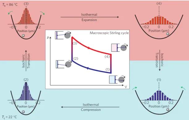
This model was experimentally realized by Blickle and Bechinger in 2012 [36]. They realized the harmonic potential with the help of optical tweezers [42] and instant heating of the viscinity of the Brownian particle with a laser absorption technique [43]. The experimental protocol is demonstrated in Fig. 2.4, which is adapted from the original paper [36].

After the first realization of a micron-sized heat engine, several colloidal heat engines were also realized by experimentalists such as a Brownian Carnot engine [37] and microscopic steam engine [38].

Figure 2.4: Schematic comparison of a macroscopic Stirling cycle and its

realization in a colloidal system. (1) The particle is initially in a low-stiffness

trap and the system is initially kept at Tc = 22◦C. Then the stiffness is increased

to operate an isothermal compression at low temperature and the cycle reaches (2). This process is followed by an isochoric heating, where the stiffness is kept constant but the temperature is increased to Th = 86◦C and the cycle reaches (3).

After that, isothermal expansion is operated by decreasing the stiffness back to its original value while the temperature is kept constant at Th, system is reached (4)

at the end of this process. Finally, the system is brought back to its initial state by an isochoric cooling. Histograms represent the equilibrium distributions of the particle at each state inside the trap. Inset: The corresponding macroscopic Stirling engine represented with a P − V diagram. Adapted from [36].

2.2

Irreversibility, second law of

thermodynam-ics and the role of fluctuations in small

sys-tems

For a Brownian particle with stationary probability distribution function

P (x, λ) = C exp

(

−U (x,λ) kBT

)

, the free energy can be written as:

F = −kBT ln (Z) (2.19)

For a reversible process, the dissipated work can then be written as:

dWdis = dW − dF = ∂U (x, λ(t)) ∂λ dλ− kBT Z ∂Z ∂λdλ Substituting Z =∫ exp ( −U (x) kBT )

into the above equation yields:

dWdis= dλ [ ∂U (x, λ(t)) ∂λ − 1 Z ∫ exp ( −U (x, λ) kBT ) ∂U (x, λ(t)) ∂λ dx ] (2.20)

Note that the first term inside the square bracket is not deterministic, rather it depends on the position of the particle at the given time. Therefore, the dissipated work as well as the work applied to a Brownian particle during a non-equilibrium process is stochastic and trajectory-dependent. Nevertheless, we can still show that there is no dissipated work if the process is reversible.

Assume that the control parameter is changing infinitely slowly. In such case, we can assume that the particle is under the same trapping potential for a very long time. Therefore, the infinitesimal dissipated work will take the form:

dWdis = dλ [ 1 dλ/ ˙λ ∫ dλ/ ˙λ 0 ∂U (x, λ(t)) ∂λ dt− 1 Z ∫ exp ( −U (x, λ) kBT ) ∂U (x, λ(t)) ∂λ dx ] (2.21)

Note that the first term inside the square brackets is the time average and the second term is the space average of the function ∂U (x,λ(t))_∂λ . In the limit where ˙λ goes to zero, these two terms will be equal to each other due to ergodicity, and therefore; we will not have any dissipated work. Thus:

lim

˙ λ→0

dWdis= 0 (2.22)

This implies that, just like in the classical thermodynamics, a reversible ther-modynamic process can be obtained provided that the system parameters are changed infinitely slowly.

The second law of thermodynamics states that no thermodynamic process can result in a decrease in the total entropy of the universe. This was proven to be true for macroscopic systems, but it was shown by Evans that this law does not always apply to small systems [3]. They performed computational studies on a liquid under external shear and concluded that due to fluctuations comparable to the system’s thermal energy, negative entropy production can be observed for small systems at small timescales. This phenomenon was investigated by scientists on different systems within the following years and yielded consistent results [44, 45, 46, 47]. Even though the second law does no longer hold when the system has a finite number of degrees of freedom, according to fluctuation theorem the second law of thermodynamics still holds on average:

⟨dW ⟩ ≥ dF (2.23)

This phenomenon is also visible in the numerical illustration of Example 2.2. The free energy of a Brownian particle is calculated according to Eq. (2.19) and

compared with work values in single realizations. In Fig. (2.3)(d), we see that the applied work can be smaller than the change in free energy in a single realization of an isothermal process, but it is still greater in average. Of course, not only the mean values, but also the fluctuations around these average values store significant information about thermodynamic systems, which will be discussed in more detail in Chapter 3.

Chapter 3

Fluctuation Theorems

In the previous chapter, thermodynamic quantities for microscopic systems are discussed. I have shown with numerical examples that for a microscopic particle that undergoes an irreversible process, thermal fluctuations give rise to signifi-cant deviations from expected values. Even though the second law still holds on average, statistical fluctuations become increasingly crucial for small systems.

So far, only the mean values of the quantities in micro-thermodynamics have been dealt with in this thesis. Although being accurate and useful, this framework is not complete. In 1997, Jarzynski pointed out that the fluctuations around mean values contain significant information. He concluded that the work distribution for a system that is driven out of equilibrium should satisfy [4, 48]:

⟨e−(W −∆F )/(kBT )⟩ = 1 _(3.1)

where ⟨·⟩ represents ensemble average and ∆F denotes the change in the free energy of the system.

For a microscopic system, the second law of thermodynamics is not always true, but it still holds on average. This is because the trajectories that result in positive entropy production are more likely to occur than their time-reversed versions.

Crooks stated that this rate of probabilities of observing the same quantity of positive and negative entropy production under time reversal is exponentially proportional to the production of entropy along the forward trajectory [5]:

PF(+∆S) PR(−∆S)

= e+∆S (3.2)

Also, he showed that for microscopically reversible Markovian systems, proba-bility rates of observing the same forward and backward trajectories under time-reversal in an arbitrary process are given by [49]:

P (x(t), λ(t)) P (˜x(t), ˜λ(t)) = e

−βQ _(3.3)

where P (x(t), λ(t)) denotes the probability of observing a trajectory x(t) under the protocol λ(t), P (˜x(t), ˜λ(t)) denotes that for the time reversed trajectory

un-der the time-reversed protocol ˜λ and Q denotes the heat exchange between the

particle and the heat bath along the forward protocol.

An important consequence of Eq. (3.3) is the work fluctuation theorem, which is valid if the system is initially thermalized [5]:

PF(+W ) PR(−W )

= e−β(W −∆F ) (3.4)

which also implies Jarzynski equality (Eq. 3.1). After these two relations, many other fluctuation theorems have been developed such as the Hatano-Sasa relation [50] and the Hummer-Szabo formula [51].

As the theoretical framework of stochastic thermodynamics developed [29, 52], other non-equilibrium relations have also been formulated [53, 54, 55, 56]. In this section, along with Crooks fluctuation theorem and Jarzynski relation, I am going to be particularly focusing on the integral fluctuation theorem [6, 57]:

⟨ exp ( βQ− logp(x0) ˜ p( ˜x ) )⟩ = 1 (3.5)

Unlike Eq. (3.1) and Eq. (3.4), Eq. (3.5) does not require initial equilibrium. All of these non-equilibrium relations attracted great interest from experimental-ists and have been tested with experiments [7, 8, 58, 59, 11, 60, 61, 62, 9, 10, 63, 64].

In the rest of this chapter, I will explain Crooks fluctuation theorem, Jarzynski equality and the integral fluctuation theorem in detail with theoretical derivations and numerical exemplifications.

3.1

Crooks Fluctuation Theorem

In this section, I will explain in detail how Crooks obtained [49] Eq. (3.3) for Markovian systems and how this equation leads to Eq. (3.4) [5]. Then, I will il-lustrate this relation with numerical realizations under arbitrary non-equilibrium thermodynamic processes. Finally, I will conclude highlighting the first experi-mental realization of this relation.

Consider a Brownian particle in a thermal bath driven by an overdamped Langevin equation. Such a system is called Markovian as the particle’s future trajectory has no dependence on its history. Consider a Brownian particle which is held initially in a potential given as:

U (x) = U (x, λ0) (3.6)

where λ0 is the initial value of a control parameter that can be driven externally.

We start changing this control parameter at t = t0 and end the process at t = tN.

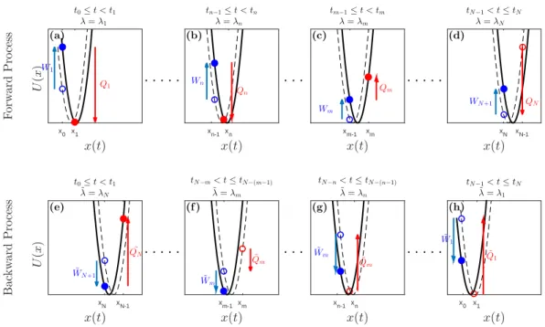
· · · · · · · · x(t) x₀ x₁ F or w ar d P ro ce ss U (x ) W1 Q1 t0≤t < t1 λ= λ1 (a) x(t) x_n-1 x_n Wn Qn tn−1≤t < tn λ= λn (b) x(t) x_m-1 x_m Wm Qm tm−1≤t < tm λ= λm (c) x(t) x_N x_N-1 QN WN+1 tN −1< t ≤ tN λ= λN (d) x(t) x N xN-1 B ac k w ar d P ro ce ss U (x ) ˜ WN+1 ˜ QN t0≤t < t1 ˜ λ= λN (e) x(t) x m-1 xm ˜ Wm ˜ Qm tN −m< t ≤ tN −(m−1) ˜ λ= λm (f ) x(t) x n-1 xn ˜ Wm ˜ Qm tN −n< t ≤ tN −(n−1) ˜ λ= λn (g) x(t) x 0 x1 ˜ W1 ˜ Q1 tN −1< t ≤ tN ˜ λ= λ1 (h)

Figure 3.1: The same forward and backward trajectories under time

reversal in a non-equilibrium process. The process starts with changing λ0

to λ1 at t = t0. Then at each ti, the control parameter is changed to λi+1. The

titles indicate the time interval of each heat exchange and the control parameter during the same time. The time when the change in control parameter occurs is represented with equality. If the change of control parameter occurs after the heat exchange, the initial position of the particle is shown by red hollow circles. If the change of control parameter occurs before the heat exchange, the final position of the particle is shown by red disks. (a) corresponds to initiation of the process, (b) and (c) correspond to arbitrary intermediate steps, (d) corresponds to conclusion of the process. The reverse protocol is also shown in the same manner in (e),(f),(g) and (h), respectively. Note that ˜Wi =−Wi and ˜Qi =−Qi

for the corresponding forward and backward steps.

ΛF ≡ λ0 ==⇒ t=t0 λ1· · · λn ==⇒ t=tn λn+1· · · λN ==⇒ t=tN λN +1 . (3.7)

The limit N → ∞ corresponds to the continous case. We denote a certain trajectory, X as follows:

The process begins at time t = t0, when the control parameter is changed from λ0 (dashed line) to λ1 (solid line) as shown in Fig. 3.1(a), when W1 work (blue

arrow) is applied on the particle. Then the particle fluctuates inside the potential under control parameter λ1 until t = t1 while exchanging Q1 heat (red arrow)

with the heat bath. This process is iterated similarly, two intermediate steps are shown in Fig. 3.1(b) and Fig. 3.1(c). Finally, the particle reaches its final position

xN at t = tN having exchanged QN (red arrow) amount of heat with the bath,

when we change λN (dashed line) to λN +1 (solid line) and thus apply WN +1(blue

arrow) amount of work, shown in Fig. 3.1(d).

Given that the particle is initially at x0 at t = t0, the probability of observing

the trajectory X can be written a product of conditional probabilities:

PF(X) = p [x1(t1)| x0(t0)]_λ1···p [xn(tn)| xn−1(tn−1)]_λn···p [xN(tN)| xN−1(tN−1)]_λN

(3.9)

Now consider we operate the time-reversed protocol ΛR, which starts with λN +1 and ends with λ0, opposite to ΛF:

ΛB ≡ λN +1==⇒ t=t0 λN · · · λn+1 ==⇒ t=tn λn· · · λ1 ==⇒ t=tN λ0 . (3.10)

Let us find out the probability to observe the reversed trajectory under the reversed protocol. Similar to Eq. (3.9), we can express this probability given that the particle initially starts at xN:

PR( ˜X) = p [xN−1(tN−1)| xN(tN)]_λN · · · p [xn(tn)| xn−1(tn−1)]_λn · · · p [x0(t0)| x1(t1)]_λ1

(3.11) = p [x0(t0)| x1(t1)]λ1 · · · p [xn(tn)| xn−1(tn−1)]λn· · · p [xN−1(tN−1)| xN(tN)]λN

(3.12)

trajectory under the time reversed protocol: PF(X) PR( ˜X) = p [x1(t1)| x0(t0)]λ1 p [x0(t0)| x1(t1)]λ1 ···p [xn(tn)| xn−1(tn−1)]λn p [xn(tn)| xn−1(tn−1)]λn ···p [xN(tN)| xN−1(tN−1)]λN p [xN−1(tN−1)| xN(tN)]λN

Each fraction in the above equation is the rate between the forward and back-ward transitions between two states under the same control parameter. If the system is Markovian and therefore independent from its history, this ratio of probabilities will be the same as for an equilibrium state. In other words, if the particle is known to be at a certain position at a certain time, it is not important whether it has been in equilibrium or not for a Markovian system. Therefore, each fraction in the above expression can be replaced by the energy difference between the initial and final energies of the particle according to Eq. (2.11):

PF(X) PR( ˜X) = p [x1(t1)| x0(t0)]λ1 p [x0(t0)| x1(t1)]_λ1 | {z } exp(−βQ1) ···p [xn(tn)| xn−1(tn−1)]_λn p [xn(tn)| xn−1(tn−1)]_λn | {z } exp(−βQn) ···p [xN(tN)| xN−1(tN−1)]λN p [xN−1(tN−1)| xN(tN)]_λN | {z } exp(−βQN) (3.13) PF(X) PR( ˜X) = exp [−β(Q1+ Q2+ Q3+ .... + QN)] (3.14)

which leads to Eq. (3.3):

PF(X(t), λ(t)| x(t0) = x0) PR( ˜X(t), ˜λ(t)| x(t0) = xN)

= e−βQ

where Q = Q1+ Q2+ Q3+ .... + QN is the total heat exchange from the thermal

bath to the particle during the forward protocol. Note that this equation holds if the initial position is set to x0 in the forward and xN in the backward process. If

the systems are initially thermalized, we have to multiply the probability of the initial position of the required trajectory:

PF(X(t), λ(t)) PR( ˜X(t), ˜λ(t)) = e−βQ peq(x0, λ0) peq(xN, λN +1) = e−βQ exp(−β(U(x0, λ0)− Fi) exp(−β(U(xN, λN +1)− Ff) (3.15)

which leads to:

PF(X(t), λ(t)) PR( ˜X(t), ˜λ(t))

= eβ(∆U−Q−∆F ) = eβ(W−∆F ) (3.16)

This means that all the trajectories that yield the same work in a non-equilibrium process are equally likely to be reversed under time-reversed protocol if the system is initially thermalized. Therefore, we have derived Eq. (3.4):

PF(+W ) PR(−W ) = e

β(W−∆F ) _(3.17)

This equation can be easily tested since work can easily be quantified along stochastic trajectories as explained in the previous chapter. I will provide a numerical example of how Crooks fluctuation theorem can be seen in an arbitrary non-equilibrium process.

Example 3.1: Crooks fluctuation theorem in an arbitrary pro-cess

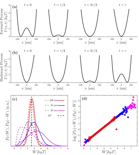
Here, I simulate a Brownian particle, which is held in a time-dependent potential: U (x, λ(t)) = Kx 4 4 λ(t) + kx2 2 (1− 2λ(t)) (3.18)

Initially I keep λ = 1 fixed for 2 seconds in order for the particle to thermalize in the trap. Then I change λ(t) from 1 to 0 within a duration

τ in the forward process, which corresponds to a transition from a double

well into a harmonic potential, shown in Fig. 3.2(a). I calculate the work done along this forward trajectories over many realizations and obtain work distribution PF(W ) for τ = 200 ms (red solid line), τ = 50 ms (blue

solid line) and τ = 20 ms (magenta solid line), as shown in Fig. 3.2(c). After that, I do the same operation for the reverse protocol: I keep λ = 0 for 2 seconds for relaxation and change λ(t) from 0 to 1 within the same

τ values, as shown in Fig. 3.2(b). Then I find the distribution of the

work done on the particle along the time reversed protocol PR(−W ) for τ = 200 ms (red dashed line), τ = 50 ms (blue dashed line) and τ = 20 ms

(magenta dashed line); as shown in Fig. 3.2(c). The rates of applied work in the forward processes and the extracted work in the backward processes are computed and displayed in Fig. 3.2(d), which verifies Eq. (3.4). This example shows that, as we drive systems between equilibrium posi-tions faster, the process becomes more and more irreversible as you can see from splitting work distributions along forward and time-reversed re-alizations for small driving times. Nevertheless, the Crooks fluctuation theorem holds true no matter how fast or slow we change the parameters, as shown in Fig. 3.2(d).

x [nm] -150 0 150 F or w ar d P ro ce ss U (x ,t ) [kB T ] 0 2 4 6 8 (a) t = 0 x [nm] -150 0 150 0 2 4 6 8 t = τ /3 x [nm] -150 0 150 0 2 4 6 8 t = 2τ /3 x [nm] -150 0 150 0 2 4 6 8 t = τ x [nm] -150 0 150 B ac k w ar d P ro ce ss U (x ,t ) [kB T ] 0 2 4 6 8 (b) t = 0 x [nm] -150 0 150 0 2 4 6 8 t = τ /3 x [nm] -150 0 150 0 2 4 6 8 t = 2τ /3 x [nm] -150 0 150 0 2 4 6 8 t = τ W [kBT ] 0 1 2 3 4 5 6 7 8 PF (W ), PR (− W ) [n .u .] τ= 200 ms τ= 50 ms τ_{= 20 ms} ∆F (c) W [kBT ] 0 1 2 3 4 5 6 7 lo g [PF (+ W )/ PR (− W )] -2 -1 0 1 2 3 4 5 (d)

Figure 3.2: Verification of Crooks fluctuation theorem in an arbitrary

process. (a) The forward protocol is demonstrated. Initially the particle is

held in a bistable potential and the potential changes into a harmonic potential within time τ . (b) The backward protocol is demonstrated; this is the opposite of the protocol shown in (a) as explained in the example 3.1. (c) Resulting work distributions in the forward (solid lines) and backward (dashed lines) processes for different driving time τ . Note that no matter how fast we operate the pro-cess, PF(+W ) and PR(−W ) are equal at the value of the change in free energy

∆F (black dashed line). (d) The rate of probabilities of the applied work in the forward protocol and extracted work in the backward protocol. For various durations of the protocol, Eq. (3.4) is verified. Work distributions are obtained by repeating the protocols 10 million times. Matlab code that produced these results is provided in appendix B.

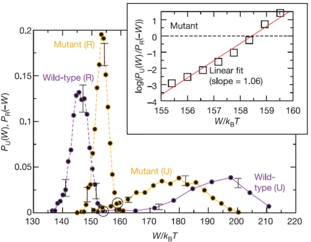
Figure 3.3: Experimental verification of Crooks fluctuation theorem. The wild-type and mutant single RNA molecules are attached to a bigger col-loidal particle and stretched by optical tweezers. By repeating the forward proto-col (Unfolding, continuous lines) and backward protoproto-col (refolding, dashed lines) many times, histogram of work values obtained. Wild type pulling experiments were repeated 900 times (purple) and mutant type pulling experiments were re-peated 1200 times (orange). Black circles mark the work values where PU= PR.

The error bars represent the reproducibility of the data via repetition of the ex-periment. Inset: The linear behaviour of . Adapted from PU/PR with respect to W , in agreement with Eq. eq:WFT. Adapted from [8].

The first experimental verification of Crooks fluctuation theorem was per-formed by RNA stretching experiment with optical tweezers [8]. They verified Eq. (3.4) by measuring the work applied on a colloidal particle that is attached to an RNA molecule. They measured work values both in unfolding (forward) and refolding (backward) processes. The resulting work distribution did not only verify Crooks fluctuation theorem, but also enabled the authors to identify the free energy difference between folded and unfolded RNA molecules. Also, from

the work distribution they were able to differentiate between wild type and mu-tant RNAs. These results are shown in Fig. (3.3), which is adapted from the same work [8].

3.2

Jarzynski equality

In this section, I will give one of several different proofs [35] of Jarzynski equal-ity, which will be followed by a numerical illustration. Then I will give a short discussion about the importance and the impact of this relation. Finally, I will conclude by highlighting an experimental verification of this equation.

Assume that we are looking for the following average in a non-equilibrium process:

⟨exp (−βW )⟩ =

∫

exp (−βW ) PF(W )dW

Here, PF(W ) is the probability distribution of applying W amount of work along

the forward non-equilibrium process. Substituting PF(W ) from Eq. (3.4)

imme-diately solves the RHS of the above equation:

⟨exp (−βW )⟩ = ∫ exp (−βW ) PR(−W ) exp [β(W − ∆F )] dW (3.19) = ∫ exp (−β∆F ) PR(−W )dW (3.20)

where exp (−β∆F ) is a constant and can be taken outside of the integral. The rest is just the sum over all probabilities of the work applied during backward process, which is trivially 1 according to normalization. Therefore, we have obtained the Jarzynski equality:

⟨exp (−βW )⟩ = exp (−β∆F ) (3.21)

Please note that this relation is alvo valid only if the system is initially at thermal equilibrium. Hatano and Sasa [50] formulated a generalized version of

Jarzynski equality when a system is not initially in an equilibrium state but in a non-equilibrium steady state. This relation is very useful as it relates the free energy differences between two equilibrium states if the work distribution is known. One important property is Eq. (3.1) holds no matter how fast or irreversible we perform the driving of the potential.

Another important property of the Jarzynski equality is that one can recon-struct the free energy landscape of all the intermediate states during a non-equilibrium process [51, 55]. Assume that the process starts at t = t0 from the

control parameter λ0 and ends at t = tf with λf. At any internediate time t, we

can write:

⟨exp (−βW (t))⟩ = exp(−β∆Fλ(t),λ0

)

(3.22)

Eq. (3.22) permits one to find out the free energy difference between the ini-tial state and any of the intermediate states. I will show a numerical example depicting how Eq. (3.1) and Eq. (3.22) work in a time dependent harmonic trap.

Example 3.2: Jarzynski relation and free energy reconstruction

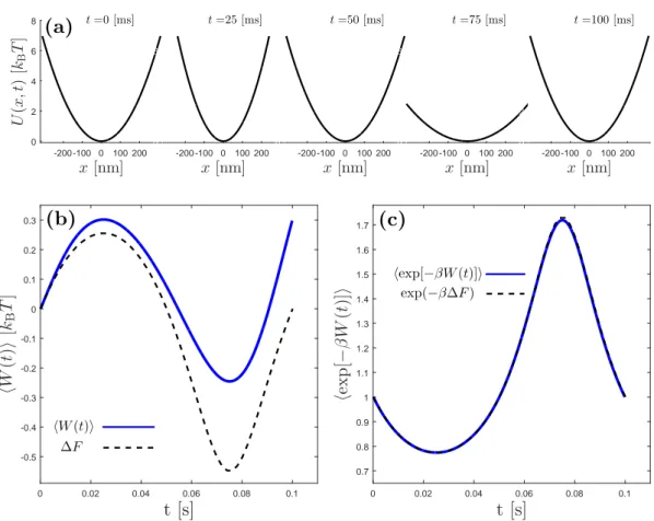
Consider that we have a Brownian particle in a thermal bath that is kept in a time dependent harmonic potential:

U (x, λ(t)) = 1

2k[3 + 2sin(ωt)]x

2 _(3.23)

where the trap stiffness changes in a sinusoidal manner. This process is shown in Fig. 3.4(a). The applied work on the particle is averaged over many realizations of the same protocol. The average applied work on the particle as a function of time is shown in Fig. 3.4(b), which is in agreement with the second law. I also verify Eq. (3.1) and Eq. (3.22) by taking the exponential average of the work applied as a function of time and comparing this to the Boltzmann weighted change in free energy, as shown in Fig. 3.4(c).

In conclusion, if the work distribution is known as a function of time for a non-equilibrium process, one can identify free energy differences between initial and final states employing Eq. (3.1), or can reconstruct the whole free energy landscape of the process as a function of intermediate states employing Eq. (3.22).

Jarzynski equality was first verified in 2002 [7] using an RNA stretching exper-iment. Such an operation can be performed by linking RNA to a greater colloidal particle and employing optical tweezers [65, 42] to stretch RNA and photonic force microscopy to analyze forces [66]. Also, this relation has been tested for single molecules [59, 9, 58, 8], mechanical oscillators [10], electronic systems [64] and colloidal particles in non-harmonic potentials [11]. Also, it is tested and veri-fied for quantum systems, where work measurements were done on a trapped ion system that was thermalized by phonons [62]. As an example, I adapt the results from a single molecule strecthing experiment [59], where the authors stretched a titin I27 molecule at different speeds and succesfully recovered the same free energy profile. These results are shown in Fig. 3.5.

x[nm] -200 -100 0 100 200 U (x ,t ) [kB T ] 0 2 4 6 8 (a) t=0 [ms] x[nm] -200 -100 0 100 200 0 2 4 6 8 t=25 [ms] x[nm] -200 -100 0 100 200 0 2 4 6 8 t=50 [ms] x[nm] -200 -100 0 100 200 0 2 4 6 8 t=75 [ms] x[nm] -200 -100 0 100 200 0 2 4 6 8 t=100 [ms] t [s] 0 0.02 0.04 0.06 0.08 0.1 hW (t )i [kB T ] -0.5 -0.4 -0.3 -0.2 -0.1 0 0.1 0.2 0.3 hW (t)i ∆F (b) t [s] 0 0.02 0.04 0.06 0.08 0.1 he x p [− β W (t )] i 0.7 0.8 0.9 1 1.1 1.2 1.3 1.4 1.5 1.6 1.7 (c) hexp[−βW (t)]i exp(−β∆F )

Figure 3.4: Illustration of Jarzynski equality in a time-dependent

har-monic trap. (a) The protocol is sketched. First, the stifness is increased, then

decreased and then finally taken back to its initial vaue. This protocol is quan-titatively explained in example 3.2. (b) The average work applied as a function of time during the process described in (a). Note that in average, one applies greater work than the change in free energy in an irreversible process. (c) Verifi-cation of Jarzynski equality. The Boltzmann weighted exponential average of the work applied follows exactly the Boltzmann weighted exponential of the change in free energy. The work values are averages over 100000 realizations of the same protocol. The Matlab code that produced these results are provided in appendix B.

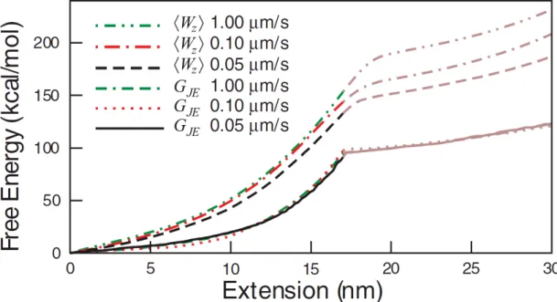
Figure 3.5: Experimental free energy reconstruction using Jarzynski

equality Estimating free energy profile using Jarzynski estimator (Eq. (3.22)).

Single molecule stretching experiments were carried out on a titin I27 at different pulling velocities. Note that as the pulling velocity increases, the process is more irreversible and therefore the average work applied is also increases. However, the estimated free energy profiles with Jarzynski estimator always gives the same free energy profile no matter how fast the molecule is pulled. Adapted from [59]

3.3

Integral Fluctuation Theorem

Here, I will demonstrate the integral fluctuation theorem [6], which concerns the heat exchange between a system and the heat bath rather than the work applied. I will begin with giving an analytical derivation.

Let us recall Eq. (3.3):

PF(X(t))/p(x0,λ0) z }| { PF(X(t), λ(t)| x(t0) = x0) PR( ˜X(t), ˜λ(t)| x(t0) = xf) | {z } PR( ˜X(t))/p(xf,λf) = e−βQ

PF(X(t)) PR( ˜X(t)) = e −βQp(x0, λ0) p(xf, λf) = exp [ − ( βQ− log p(x0, λ0) p(xf, λf) )] PF(X(t)) exp [ βQ− log p(x0, λ0) p(xf, λf) ] = PR( ˜X(t)) (3.24)

We can multiply both sides with dX and integrate:

∫ exp [ βQ− log p(x0, λ0) p(xf, λf) ] PF(X(t))dX = ∫ PR( ˜X(t))dX

note that dX = d ˜X because ˜X is the reversed trajectory of X. Therefore,

we have an average over all possible trajectories on the left hand side, and a probability summation on the right hand side:

∫ exp [ βQ− p(x0, λ0) p(xf, λf) ] PF(X(t))dX = ∫ PR( ˜X(t))d ˜X | {z } 1 ⟨ exp [ βQ− p(x0, λ0) p(xf, λf) ]⟩ = 1 (3.25)

Note that this relation does not require an initial Boltzmann distribution, the system is not required to have reached an equilibrium state before the driving process. Under certain assumptions, this equality may simplify to the Hatano-Sasa relation or Jarzynski equality, but this is a universal equality that one can employ without any assumptions about the initial probability conditions [57, 34].

Chapter 4

A non-Markovian environment:

Active matter

So far, I have discussed the stationary distributions and non-equilibrium rela-tions of thermal systems, which are Markovian and therefore, microscopically reversible. Active systems, however, are subject to active noise that may arise from biological media or artificial activity like self-propelled particles. Thus, these systems are intrinsically out of equilibrium and presumed to be examined only in the framework of non-equilibrium physics [67, 68, 32, 69, 70]. There have been several studies in which scientists have discussed to what extend statistical physics can be applied to such active systems [12, 13]. In this section, I will give an overview of how active systems can be characterised by the properties of their activity and under which conditions their activity could be mapped to thermal systems with enhanced effective temperatures.

An active Brownian particle is able to self-propel [71]. Most common agents that come across in nature that could be categorized as an active Brownian particles are swimming microorganisms like Escherichia coli [72]. Some microor-ganisms in nature may exhibit run-and-tumble motion, which corresponds to swimming in a certain direction for a while and stopping for a while to reorient itself [73], which have similar statistical behaviour and difusion characteristics to

smooth swimmers [74]. Such an activity can also be realized with an artifical swimmer which creates asymmetry around its viscinity to induce self-propulsion [75]. Such a mechanism can be realized with various techniques such as chem-ical asymmetry [76, 77, 14], thermophoresis [78] or critchem-ical demixing [79]. A self-propelling particle propels itself with a constant force which results in the following set of Langevin equations:

˙x = V cos(ϕ)√2DTWx(t) (4.1)

˙

y = V sin(ϕ)√2DTWy(t) (4.2)

˙

ϕ =√2DRWϕ(t) (4.3)

where ϕ represents the orientation of the self-propelled particle, which is subject to rotational diffusion. Here, Wx, Wy and Wϕ are white noises with zero mean

and unitary variance. The mean square displacement of such a swimmer in 2 dimensions can be analytically derived as [80, 14]:

MSD(t) = [4DT + V2τR]t + V2τ_R2 2 [ e−2tτR − 1 ] (4.4)

while τR represents the characteristic timescale of particles rotational motion.

This leads to 3 different phenomenon to be observed for an active particle at different timescales:

1. Standart diffusive regime, when t << τR. The resulting MSD will take the

form

MSD(t) = 4DTt

Here, the slope of MSD-t graph will be 1 as it performs regular diffusion.

2. Superdiffusive regime, when t≈ τR. At this timescale, one would need the Eq. (4.4) to explain fully the dynamics. In this regime, the slope of MSD-t graph will be between 1 and 2.

3. Enchanced diffusion regime. In the limit when t >> τR. Here, MSD of the

particle will be given as:

Figure 4.1: Mean square displacement (MSD) of active Brownian

par-ticles and effective diffusion coefficients. (a) Numerically calculated and

(b) theoretical MSD for active Brownian particles with velocity V = 0 µm s−1 (circles), V = 1 µm s−1 (triangles), V = 2 µm s−1 (squares) and V = 3 µm s−1 (diamonds). For passive Brownian particles (V = 0 µm s−1, circles) the motion is always diffusive, while for active Brownian particles the motion is diffusive with diffusion constant DT at very short timescales, (τ << τR), ballistic at

interme-diate timescales (τ ≈ τR), and again diffusive but with an enhanced diffusion constant at long time scales (τ >> τR). Adapted from [13].

Here, the slope of MSD-t graph will go back to 1, and diffusion properties of the system can be represented with an effective temperature Teff = T +γV

2_τ

R

4kB

These 3 regimes are demonstrated nicely in a recent review paper, which is shown in Fig. 4.1. Please note that these categorization of timescales ignores the inertial timescales when t≈ m/γ, where m/γ is the momentum relaxation time of the Brownian particle. For such ultra short timescales, particle exhibits ballistic motion and therefore, the slope of MSD-t curve is expected to be 2. However, for typical soft matter experiments, this number corresponds to fraction of a microsecond, which is not accesible for standart position measurement techniques like digital video microscopy or interferometry [42]. Nevertheless, this regime has been explored experimentally by using high-bandwidth quadrant photodiodes [81, 82, 83].

immersed in an environment in which there are plenty of active particles, e.g. motile bacteria which is called an active bath [84, 85]. All these systems are called non-Markovian as in short timescales when t and τRare comparable to each

other as the particle’s velocity becomes correlated, which results in the violation of equilibrium conditions and time reversal symmetry. Under such conditions, lots of interesting non-equilibrium phenomenon are observed like crowd control [17], directed transport [86, 18, 87, 88, 89], cluster formation [90, 91, 92] and energy harvesting from a single bath [93, 94]; all of which are not possible to observe in a Markovian environment.