162 IEEE TRANSACTIONS ON INFORMATION THEORY, VOL. 36, NO. 1, JANUARY 1990
An Implementation of Elias Coding for
Input-Restricted Channels
ERDAL ARIKAN. MEMBER, IEEEAhstrurt -An implementation of Elias coding for input-restricted chan- nels is presented and analyzed. This is a variabk-to-fixed length coding method that uses finite-precision arithmetic and can work at rates arbitrar- ily close to channel capacity as the precision is increased. The method offers a favorable tradeoff between complexity and coding efficiency. For example, in experiments with the 12, 71runlength constrained channel, a coding efficiency of 0.9977 is observed, which is significantly better than what is achievable by other known methods of comparable complexity.
I. INTRODUCTION
Ever since Shannon [ l , p. 361 formulated and studied input- restricted channels, many coding methods have been proposed for such channels; the reference section proGdes a partial list. We present another method, based on Elias coding, which may be of interest since it can achieve extremely high coding efficiencies using little memory and computation.
The idea of using Elias coding for input-restricted channels is not new, though the earlier codes were presented under the name of arithmetic coding [4], [5], [6]. The primary interest in [4], [5] was in fixed-rate implementations. Here, we consider a variable- to-fixed-length implementation that is fixed-rate only in a certain asymptotic sense. It return for giving up the strict fixed-rate property, a favorable tradeoff is obtained between coding com- plexity and efficiency, as demonstrated by experimental and analytical results.
The relation between Elias coding and the code here is a special case of the duality between source coding (data com- paction) and coding for input-constrained channels (data transla- tion). The decoder for a data-translation code is an encoder for a data-compaction code: it removes the structural redundancy that is present in the constrained channel sequence. This relationship was stated and exploited in [4], [5], and more recently in [16]. For the code here, the decoder is an Elias encoder, more exactly a
finite-precision floating-point implementation of Elias coding, similar in some respects to that in [15]. (For Elias coding and its variants, see [14].)
The main results of this correspondence are contained in Section IV. Sections I1 and 111 contain definitions, conventions,
and some background results. Section V contains complementary remarks on the algorithm.
11. CONVENTIONS AND DEFINITIONS
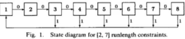
We consider only input-restricted channels that can be pre- sented by finite state diagrams. An example of such a channel is the [2, 71 runlength constrained channel, presented by the state diagram in Fig. 1. (Runlength constraints arise, e.g., in magnetic recording applications. For details, see, e.g., [13].) Each edge in Fig. 1 is labeled by a 0 or a 1, the input letters for this channel. A 0-1 sequence is admissible as an input to the [2, 71 channel iff it can be generated by a walk through the state diagram. It will be noted that runlengths of 0 in admissible sequences are bounded 4
I
Manuscript received December 7. 1987: revised May 13, 1989. This research was supported in part by Joint Services Electronics Program under contract N00014-84-C-0149. This correspondence was presented in part at the IEEE International Symposium on Information Theory, Kobe, Japan, June 1988.
T h e author is with the Department of Electrical Engineering, Bilkent Uni- versity. P.K. 8 , 06572, Maltepe, Ankara, Turkey.
I E E E Log Number 8933104.
Fig. 1. State diagram for [2, 71 runlength constraints.
between 2 and 7, and being in state i implies that the current runlength of 0 is i
-1.
There may be several reasonable ways of presenting an input- restricted channel by a state diagram. For our purposes any such presentation is acceptable as long as it has the properties of being simple and deterministic. A state diagram is said to be simple if for each pair of (not necessarily distinct) states i and j , there is at most one edge from state i to state j . A state diagram is said
to be deterministic if, for each state, the labels on edges emerging from that state are distinct.
Note that, if one is given a sequence of edge-labels through a deterministic state diagram and the initial state is known, one can then determine the sequence of states visited by the walk. (This notion was expressed by the terms unifilar in [2] and, in a somewhat weaker form, by right-resolving in 191.)
It is easy to see that if an input-restricted channel can be presented by a finite state diagram, so can it be by a simple, deterministic one. So, the restrictions we have imposed on state diagram presentations do not exclude any channels. We shall, however, exclude from consideration those channels that cannot be presented by irreducible state diagrams. A state diagram is
said to be irreducible if there exists a directed path from each state to each other state. Channels that are not irreducible are not of particular interest; they are best studied in terms of their irreducible components. Henceforth, we shall assume that the state diagram under consideration is finite, simple, deterministic, and irreducible.
Let us note that the restriction to simple state diagrams is made only to simplify the notation; the coding method presented here can be applied to nonsimple state diagrams after minor changes. The restriction to deterministic state diagrams is essen- tial for decodability, though that too can be relaxed somewhat (to what is called right-resolving in [9]).
We shall label the states by integers 1 through S , where S denotes the number of states. We shall let t , . , , 1 I i, j I S ,
denote the number of edges from state i to state j . Thus, t , , , will be either 0 or 1 since we consider only simple state diagrams. The
matrix T = ( t , , / ) will be called the state transition matrix. We shall let l , . , denote the channel symbol labeling the edge from state i to state j ; if there is no such edge, 1,.
,
will be undefined.111. MAXENTROPIC PROBABILITIES
AND CHANNEL CAPACITY
Let A be the largest positive eigenvalue of T , the staie-transition matrix for some input-restricted channel. Let ( B , , 1 I i I S ) be
an eigenvector belonging to A : T B = A B . (By the Frobenius
theorem for irreducible, nonnegative matrices [3, p. 531, B is unique up to a scaling constant, and one may assume that B, > 0 for all i.)
Shannon [ l , p. 581 showed that the entropy of the input to an input-restricted channel is maximized by a source that visits the states of the constraint diagram according to the following Markovian transition probabilities:
p , , / = t i , i B j A - ' / B , .
IEEE TRANSACTIONS ON I N F O R ~ ~ A T I O N THEORY, VOL. 36, NO. 1. J A N U A K Y 1990 163
i
These transition probabilities are called maxentropic, and the resulting maximum entropy is calculated to be log A.
Shannon 11, p. 371 also showed that the capacity of an input- restricted channel is given by C = log A. Thus, in order to use this noiseless channel at the maximum possible rate C, one must maximize the entropy of the channel input. This suggests that the output of an encoder working at a rate close to channel capacity should, in some sense, approximate the . maxentropic Markov chain. The algorithm presented in the next section tries to achieve this as best it can under the limitations of finite-precision arith- metic.
IV. THE ALGORITHM
The algorithm presented here is a variable-to-fixed-length slid- ing-block code, which in each encoding cycle accepts a variable number t of new data bits into the encoder and sends out one
channel symbol. The encoder thus maps a data sequence
d, ,
.
..
, d, to a code sequence x,, . . . , x , ~ . The decoder processes the code sequence x, ,. . .
, x , ~ and generates d,, . . . , d , K , the original data sequence except for a tail of K bits. The number K of undecodable bits is data-dependent, but always upperbounded by r, the length of registers used by the algorithm. Thus, by appending to the original data sequence a fixed tail of r bits, one can ensure the decodability of all data bits. Since we shall be primarily interested in the asymptotic performance of the algo- rithm as L goes to infinity, we shall ignore these end-effects.In order to apply the algorithm to an input-restricted channel, we first fix a state-diagram presentation. Then, we choose a matrix of transition probabilities ( p , , / ) on this state-diagram so that p , , = 0 whenever t,, I = 0 , and C.:=,p,, I =1, all i. The
algorithm can work with any such set of transition probabilities, but what is intended is to choose the ( p , , , ) as close to the maxentropic probabilities as possible within finite precision. It is aimed to have the encoder behave like a Markov chain (in its transitions from one state to another during the encoding pro- cess) with the chosen transition probabilities when the encoder input is a symmetric Bernoulli process (independent, equiproba- ble bits).
A pseudocode for the algorithm is shown next. procedure encode((F;. ( I , . r , so);
begin
begin{ initialization}
,y := s(,;
.”
:= 0; z := 2’- 1’ w := z - y ’ u : = Z : : = , d , 2 ’‘
end{ initialization} while not end-of-data do begin { encodingcycle} determine the least i such that
q , ,
-E , ,
I > 0 and.v
+ I w F . , l >
U ; output the next code letter x = I , , , ;z : = ? , + l w F , , , l ;
.v:=.v+1wq,,
1 1 ; t := t(.v,
z ) :shift t 0’s into register y : shift t 1’s into register z ;
shift the next t data bits into register U ; w : = z - y. s : = l
end { encodingcycle } end.
procedure decode((
5,
/), ( I , , /), r, so): beginbegin{ ini tialization}
. 3
s : = s . (,, . V : = 0; z := 2’ - 1; M: := z - y
end(initia1ization)
while not end-of-code-sequence do begin{ decodingcycle}
input the next code letter x;
determine the state i such that /,,, = x; z := .V
+
I
w e , ~ J ;.
v:=
.v + l w q , )
1 1 ; t := t (’.
z ) ;output the leftmost t bits of register y ;
shift t 0’s into register y ;
shift t 1’s into register z ;
end{ decodingcycle} end.
w := z - V; := i
We shall first explain some variables and operations that appear in this pseudocode. For each pair of states, there is a cumulative probability defined by
By convention. we take
c,,,
= 0 for all i.The variables U , y , and z represent r-bit, right-to-left shift- registers. Register U holds a window of r data bits: U = d,,+ .
.,
d,,.
, , where h is the number of bits that have been processed by the encoder until then, and left the system. The contents of register U are also treated as the integer U =1:-
,d,, *(2‘ ‘. In the same manner, registers y and z are treated as both bit sequences and integers. Thus, setting z = 2’- 1 isequivalent to loading register z with r 1’s. Likewise, setting U =Z:=,d,2’
‘
loads register U with the first r data bits.The function t( y , z ) gives the length of the common (left) prefix of registers y and z (e.g., if y = 001001 and z = 001110 (with r = 6), the common prefix is 001 and t ( y , z ) = 3).
The shift operation on registers is best explained by an exam- ple: If U = 001010 ( r = 6), then executing “shift 111 into register U ” results in U = 010111.
To explain how the algorithm works, let us indicate the value of a variable at the end of encoding cycle n by the subscript n
(e.g., y,,, s,), etc.). Let the subscript 0 indicate initial values. The algorithm works by generating, in effect, a sequence of intends I,, = [ J ! , z , , ] , n 2 0, with the property that ytj 5 u , ~ I z ~ , . In the
nth encoding cycle, the initial interval
I,,~-
I = [ j ; ,,,
z , ,, I
is divided into subintervals so that there is one subinterval for each state. The subinterval for state i is empty ifit equals
P\,,
,
,
q,, ,
,
-E,,
I , - I = 0 ; otherwise,What is aimed here is to allocate a fraction p,,, I , / of the initial
interval to state i. These subintervals may overlap at their end- points, but what matters is that they cover all integers in I,,
-,.
(With a more complicated rule, one could guarantee disjoint subintervals and slightly improve the coding efficiency.) The encoder sets s,, equal to the least i such that U,,-, lies in the subinterval for state i. The symbol x,, = I,,?- I , ,,, is then sent to thechannel.
Let us now look at the situation from the decoder’s point of view. Suppose that the decoder has kept up with the encoder and
~
164 IEEE TRANSACTIONS ON INFORMATION THEORY, VOL. 36, NO. 1, JANUARY 1990
14 12 10 8 6 4 2 0 53 54 55 56 57 5 8 59 60 6 1 62 63 64 65 6 6 6 7 68 69 70
Fig. 2:. Histogram of number of decoded digits minus 5100 for algorithm.
is in possession of y,, ~ z,,
,,
and s , , ~ After observing x,,, thedecoder can determine s,, (since the state diagram is determinis- tic), and hence, y,,, z,,, and the leftmost
I ,, = t ( Y,, I +
1
w,, ~ 1 F , , - ~ . ,,,- 1 1 Y,,- 1 +1
~9,- 7.J
( 4 )bits of U , , This explains why the encoder can drop, as it does, the leftmost t,, bits of register U , thus making room for the upcoming t,, data bits. The updating rule for registers y and z
ensures that the inequality y,, I U,, I z,, is satisfied going into the next cycle; so the process can continue indefinitely.
Thus the number of data bits that the decoder is able to decode
after observing the first n code letters is given by
T,
=t ,
+
. . .
+
t,,. The question that arises is whether the code here isasymptotically fixed-rate, i.e., whether R,, = T , / n converges as n
goes to infinity to a fixed rate R for all data sequences. (In such
limits, we assume that L , the number of data bits, is infinite.) Unfortunately, this is not so. However we shall see later in this section that, if each data sequence of a fixed finite length is assumed equally likely, then the set of all infinite-length data sequences for which the previous statement is false has total probability zero.
4
I
A . A n Experimental Result
We applied the algorithm to the [2, 71 runlength constrained channel presented in Fig. 1 . The numbers
(4,
,) were based on the following transition probabilities: p 3 , ] = 0.34, p4,1 = 0.36, p s . l = 0.40, ph,l = 0.46, P , . ~ = 0.59, which were obtained byrounding off the maxentropic transition probabilities. The regis- ter length was r = 8.
We carried out the experiment 100 times. In each run the input to the encoder was a simulated symmetric Bernoulli sequence. The encoder was run until it produced N = loo00 code letters,
which were then processed by the decoder, and the number T, of decoded bits was recorded. Fig. 2 shows the frequency of occur- rence of the observed values of T,.
We observe that the sample mean of the rate R , = T , / N
equals 0.516165, which is within 0.23% of the channel capacity C = 0.517370 . . . for the [2, 71 channel (see [13] for the capacity).
We also observe that the spread of the observed values of T, around the sample mean is, relatively speaking, quite small, suggesting some statistical regularity. The analysis that follows helps to explain these observations.
B. Statistical Analysis of the Algorithm
For the statistical analysis, we assume that the data sequence is a symmetric Bernoulli process. We first sketch a proof that R ,
converges almost surely as N goes to infinity.
The proof is based on the observation that the sequence
( u , ~ : n 2 0), where U,, = (s,,, y,,, z,,), is a Markov chain with time- invariant transition probabilities. This follows from the facts that
U,, is a function of U , , - , and u , ! - ~ , and that U,,-, is uniformly distributed (equally likely to take on any integer value) on the interval [y,, I , z,, , ] , regardless of the path taken to reach the state U,, I . (These statements can be proved easily by induction.)
Since the random variable t,, is a function of u , ! - ~ and U,,, i.e.,
t,, = t ( U,, U,,), we can write
R , = 1 / N
c
t , , =c
f N ( U , ~ ' ) t ( U , ~ ' ) ( 5 )l s r r s i v ( 0 , o ' )
where the random variable f, ( U , 0 ' ) equals 1 / N times the num-
ber of transitions from state U to state U' during the first N
transitions in the sequence ( U , , ) . Since (U,,) is a Markov chain with finitely many states, the times at which a transition occurs from state U to state U' form a renewal process; hence, we have,
almost surely as N goes to infinity (e.g., [17, p. 290]),
f b ( u , u ?
=
%rC,d ( 6 )where T, is the reciprocal of the mean recurrence time of state U ,
and r,,,, is the transition probability from state U to state U ' .
From ( 5 ) and ( 6 ) , we have, as N goes to infinity,
R,%R = r , r , , , . t ( u , a ' ) .
(
7 )( 0 . 0 ' )
We have thus shown that the coding rate asymptotically ap- proaches a constant R for almost all data sequences.
Next, we present an analysis, though inexact, provides insight
into why and under what conditions we may expect R to be close
to the channel capacity. We begin by noting the following recur- sive relation:
w,, = z,, - y,,
=
(
1
w,, - IF,, ,
,,,I
-1
w,, - 1e.-,,
S" - 11)
2"+
zrp8
- 1 . (8)w,,
=
w,r-lP\"~l.5"2'n ( 9 )The algorithm aims at having \
within the limitations of finite-precision arithmetic. The idea is to have, as a consequence of the preceding equation,
W k ~ ~ ) P , , , . , , P ~ , . ~ ~ . . . P ~ N I . . N 2 T N . ( 1 0 )
wh. = wo( B , N / B , o ) 2 - N C t T ~ , ( 1 1 )
For ( p , ,) approximately maxentropic, this implies
where C is the channel capacity. Since 1 I w, I 2' - 1, it follows
that, for large N ,
IEEE TRANSACTIONS ON INFORMATION THEORY, VOL. 36. NO. 1. JANUARY 1990 165
Thus to the extent that the previous approximations are valid for the state sequence (s,!) corresponding to a data sequence, the coding rate for that data sequence will be close to the channel capacity. The most effective way of ensuring the validity of these approximations for a large fraction of data sequences is to choose
r , the register size, suitably large.
Note that in the limit of infinite precision, the above approxi- mations are exact and the code is truly fixed-rate. The algorithm deviates from being fixed-rate as the precision is decreased. The experimental values of
R
I previously reported suggest that evenwith a modest precision that deviation may be kept at an insignif- icant level.
C. The Error Propugution Problem
Suppose that, instead of the entire code sequence xl, x 2 ; . ., the decoder is given x,!
,
, x,, + z, . . . . Can the data sequence stillbe reconstructed correctly allowing a finite number of initial errors? This situation arises when some of the first n symbols are
garbled by noise, or when one wishes to start decoding in the middle of an encoded sequence. In such cases, one would not like to see a catastrophic propagation of decoding errors.
Unfortunately the codes generated by the algorithm may suffer catastrophic error propagation. We now examine this problem in more detail, mention possible remedies, but propose no specific solutions.
Let U,, denote, as before, the state of the encoder at the end of
encoding cycle n. Let
4,
denote the state of the decoder at the end of decoding cycle n . We may viewe,,
as the decoders estimate of U,). Assume that x,, e,,
x,,+>, . . . is error-free.From our discussion of the decoding algorithm, it is clear that the output of the decoder at decoding cycles > n is completely
determined by
(s,,,
x,, ~,
, x,, + ?,. . .
). In other words the effect ofxl; . ., x,, on the future behavior of the decoder is completely summarized by
6,.
Thus for each possible value of4,
(there are finitely many) there is a hypothetical data sequence. One of these sequences, the one for which 3,, = U,,,
is the true data sequence. Inorder to stop error propagation, the decoder must be able to select one of the hypothetical sequences that shares a common suffix with the true sequence. (Two sequences q , CY?,
. . .
andPI,
/Iz, .. .
are said to share a common suffix if there exist k , k’such that a/\
,
=PI
+, for all i 2 1.)A straightforward, but not particularly elegant, solution to this problem is to build some structure into the data sequence (e.g., by inserting parity-check bits) so as to facilitate the elimination of false data sequences. This approach requires no major changes in the algorithm itself. Another approach is to try to modify the algorithm so that both the encoder and the decoder update their states using a next-state function with finite look-ahead and finite look-back
where k , k‘ are fixed integers. Clearly, an algorithm with such a next-state function is noncatastrophic, with a maximum synchro- nization delay of k
+
k ’ + l symbols. The algorithm here has a next-state function of the form U, = f ( ~ , ~ ~ , x , ) , which has no look-ahead, but possibly infinite look-back. We have found no clean way of modifying the algorithm so as to eliminate the potentially infinite memory from its next-state function.We should note that there are algorithms (e.g., [9], [lo]), for which the next-state function is in the form (13), with one important difference: for these algorithms, each argument of the next-state function (the terms x , - ~ ;
.
.,
x , + ~ , ) is a block of q symbols (for some fixed integer q ) from the channel alphabet.Unfortunately such a next-state function does not provide pro-
tection against misframing (i.e., incorrectly deciding the block boundaries); hence, these codes, too, are subject to catastrophic error propagation.
V. CONCLUSION
Nonfixed-rate codes require buffering if one wishes to use the channel synchronously, and one has to worry about the conse- quent buffer overflow problems. For this reason there is a bias towards fixed-rate codes in practice. Such a bias is hard to justify in systems where the source sequence is highly redundant and one uses a variable-length source code (such as a Huffman code) to remove part of that redundancy, since buffering is required then whether the channel coding is fixed-rate or not.
Fixed-rate codes do not present a buffer-overflow problem, but they may require considerably more implementation complexity. Consider, for example, the fixed-rate codes proposed in [7], [8]. and the ones pioneered by Adler, Hassner, and Coppersmith [9],
[lo],
[ l l ] . These codes are constrained to work at rational rates; and, to construct a code with rate p / q , one needs to work with aq-step state-diagram for the given channel. Since the q-step diagram contains on the order of 2‘IC states for a channel with capacity C , the implementation complexity of these codes is exponential in q. The constructions in [9],
[lo],
[ll] have an even higher complexity because they apply state-splitting (an elegant procedure invented by Marcus [12]) to the q-step diagram, result- ing in a further increase in the final number of states. The fact that the complexity is exponential in q places a practical limit on how close one can get to the channel capacity with rational rates of the form p / q .In contrast, the algorithm here never has to deal with extended channels no matter how close the desired coding rate is to channel capacity. In order to achieve higher rates, one need only run the same algorithm using a higher precision.
REFERENCES
C. E. Shannon and W. Weaver. The Murheniuricul Theory of Coninirinicu-
r i m
H. McMillan, “The basic theorems on information theory,” A t n i . Murh. Sror.. vol. 24. pp. 196-219. June 1953.
F. R. Gantmacher. The Theorr of Murrices. i d . I I . New York: Chelsea. 1959
G N . N . Martin. <;. <;. Langdon, Jr., S. J. P. Todd, “Arithmetic codes for constrained channels.” I B M J . Res. D e i d o p . . vol. 27, pp. 94-106, Mar. 19x3.
S. J. P. Todd. C;. G. Langdon. Jr.. G. N. N. Martin, “A general fixed rate arithmetic coding method for constrained channels,” I B M J . Re.i. D e i d o p . . vol. 27. pp. 107-115. Mar. 19x3.
H . Sato. “ O n the generation of run-length constrained codes by arith- me tic coding,” IEICE (1n.v. E/ectron., In/orni. Conini. Engineerr), Tech- n i u l Reporr. vol. R7. IT 87-94, pp. 25-30. 1987 (in Japanese). P. A. Franaszek. “Construction of bounded delay codes for discrete noiseless channels.” I B M J . Res. D e i d o p . . pp. 506-514, July 1982. A. Lempel and M Cohn, “Look-ahead coding for input-restricted chan-
Trun\. ln/orni. Theo?. vol. IT-28, pp. 933-937. Nov. 19x2 persmith. and M. Hassner. “Algorithms for sliding
Truns. Inforni. Theor,. vol. IT-29. pp. 5-22. Jan. Urbana. IL: Univ. of Illinois Press, 1963.
19x3.
H. Marcus. “Sofic systems and encoding data,” 16
Theor:i., vol. IT-31. pp. 366-377. May 1985.
H. H. Marcus. “Sliding-block coding for input-restricted Trun.\ lnforni. Theorr, vol. IT-34, p p 2-26. Jan. 19XX. tors and extensions of full shifts.” Monurs. Murh.. vol. XX, pp. 239-247, 1979.
A. Norris and D. S. Hlooniberg, “Channel capacity of charge-constrained run-length limited codes,” I T r u m Mug.. vol. Mag-17. pp. 3452-3455. Nov. 19x1.
zciples O / Irforniurron Theory. Reading. MA: Addi-
efficient coding system for long source sequences,”
I ) ) . Thfwri.. vol. IT-27, pp. 280-291, May 1981.
K . J. Kerpez. “ R u n length codes from source codes via maximum entropv probabilities.” Ahrrucrs of Puprrs. I E E E l n r . Synip. lnforni. Thror1,. Kobe. Japan. 19XX.
E. Cinlar, Inrrodu(.rrori 10 Srochusric ProcesAes.
Prentice-Hall, 1975.
Englewood Cliffs. N.J.