•ν'ί'ν'’’· '*-■’·« - ïj-«';··· ■■ ; il-, ■'. ·;·-'ν·" J ·,V ѵ/ г* ί *' *' ·' · · *■, ^ ,*..J> · / · .j j т ''·■' f . ' Г. ^ ■» ·!♦.-* J ·ί- t*, ,
YSff
î . s a ö ■ : ' ■ . > ■ ■ ■ ; ■ · ■ ■ ■ . ■ ■ · ■ · . А . íRtfís» A v * , A y « · ^ · ■ · . »âtÿ v > ’^S t a x ' s лАгЛ^*^'.-Л ѴГь'*.,^.л .>· ’ ■· ‘S:-·’·» S· * ' У - «.·»*·· ·>.■·'■■’■ ί·'·Τ*'·· · ·· '» -'îî *Τ*·:·' .«·· ·.«·· vH· ·*■ · . '■ ■.i'VV-Íji-'Vk % ··'^· ν,Ι,'.^Λίϊ ■ ν > · χ · · · ’■ ■ V - ’><V¿'« ' ^>*v¿V v¿¿> ..í'; . ·., •i·.·.· ■.■.·:. .··. .■ ■ •‘s ^ ’^Ííí'■ ^ .■* ■- ■' -·-,■·■ ^-! ..· \ ; V :■ .r’V.·'·. ·,.·■ :.·, .. i Τ\*·· ^Ч"ѴЗ ^’■>'· Í^í.^».v'u \ і'^·'. ·■ir.‘ .fe ’*· • 'Г'-ѵ: ' '■' '»Ф«г»'’^··· -'■^'9*rt··■it?·* '*f-4*Í7>ÁnAvv . '/«.Αλν^.4·;THE DEMAND FOR MEAT IN TURKEY ,1979-1989.
A Thesis
Submitted to The Department of Economics
and the Institute of Economics and Social Sciences of Bilkent University
In Partial Fulfillment of the Requirements for the Degree of
MASTER OF ARTS IN ECONOMICS
By
Jülide YILDIRIM
f-ίΟ
лгг
"■/55
ί6 5 0
THE DEMAND FOR HEAT IN TURKEY ,1979-1989.
A Thesis
Submitted to The Department of Economics
and the Institute of Economics and Social Sciences of Bilkent University
In Partial Fulfillment of the Requirements for the Degree of
MASTER OF ARTS IN ECONOMICS
By
I certify that I have read this thesis and in my opinion it is fully adequate,in scope and in quality, as a thesis for the degree of Master of Arts in Economics.
Assist. Prof. Dr. Erol ÇAKMAK
I certify that I have read this thesis and in my opinion it is
fully adequate,in scope and in quality, as a thesis for the degr of Master of Arts in Economics.
ee
eX
Prof. Dr. Subidey TOGAN
I certify that I have read this thesis and in my opinion it is fully adequate,in scope and in quality, as a thesis for the degree of Master of Arts in Economics.
' J Áj.
\J
Assoc. Prof. Dr. Erinç YELDAN
ABSTRACT
DEMAND FOR MEAT IN TURKEY , 1979-1989. JUlide YILDIRIM
Master of Arts in Economics
Supervisor : Asisstant Prof. Dr. Erol ÇAKMAK November 1990
In this study , pooling of time series cross sectional data is used for constructing a demand model for the Turkish Meat Market. The demand functions are simultaneously estimated by Zellner's
Seemingly Unrelated Regression Method, imposing homogeneity and
symmetry restrictions. Furthermore, a structural change test is
conducted in order to see whether there is a structural change
between the subperiods 1979-1984 and 1985-1989. It is found that
demand functions do not satisfy homogeneity restriction, implying
that there is money illusion. A structural change is found in the demand for mutton implying there is a change in consumers' preferences between two subperiods.
Keywords : Pooling time series cross sectional data. Seemingly
Unrelated Regression, Structural Change, symmetry ,homogeneity,
ÖZET
TURKÎYE ET TALEBİNİN TAHMİNİ , 1979-1989 Jülide YILDIRIM
iktisat Yüksek Lisans
Tez Yöneticisi : Yard. Doç. Dr. Erol ÇAKMAK Kasın 1990
Bu çalışmada, zaman serisi ve kesitsel verilerin
birleştirilmesiyle Türkiye Et Pazari için bir talep modeli
oluşturulmuştur. Talep fonksiyonlar! eşzamanli olarak Zeliner'in ilişkisiz Görünen Regresyon Metodu ile homojenlik ve simetri
kisitlari konularak tahmin edilmiştir. Ayrıca, 1979-1984 ve
1985-1989 dönenleri arasında bir yap sal değişin olup olnadıgını
görnek için bir Yapısal değişin Testi yapılmştır. Talep
Fonksiyonlarının simetri kısıtını sagladigi fakat honojenlik
ki sı tını saglanadıgı görülnüştür. Ayrica, koyun eti talep
fonksiyonunda bir yapısal değişiklik bulunmuştur.
Anahtar Kelimeler : Zaman serisi ve kesitsel verilerin
birleştirilmesi, ilişkisiz Görünen Regresyon Metodu, Yapisal
Değişim, Simetri, Homojenlik, Chow Testi ve F Testi.
ACKNOWLEDGEMENTS
I would like to thank to ny thesis advisor Assit. Prof. Dr.
Erol Çakmak and to the members of the thesis jury. Prof. Dr.
Subidey Togan and Assoc. Prof. Dr. Erine Yeldan.
I owe great deal of thanks to Prof. Dr. Haluk Kasnakoglu and Assoc. Prof. Dr. Zehra Kasnakoglu for their supports.
LIST OF TABLES
Table Page
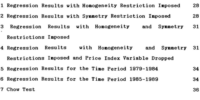
1 Regression Results with Homogeneity Restriction Imposed 28
2 Regression Results with Symmetry Restriction Imposed 28
3 Regression Results with Homogeneity and Symmetry 31
Restrictions Imposed
4 Regression Results with Homogeneity and Symmetry 31
Restrictions Imposed and Price Index Variable Dropped
5 Regression Results for the Time Period 1979-1984 34
6 Regression Results for the Time Period 1985-1989 34
7 Chow Test 36
CONTEHTS ABSTRACT ÖZET ACKNOWLEDGEMENTS LIST OF TABLES iv V Vi 111 1. INTRODUCTION
2. THEORETICAL FRAMEWORK AND RELATED RESEARCH 2.1 Demand Functions
2.2 Related Research on Demand for Meat
3 8
3. RESEARCH METHODOLOGY
3.1 Some Consideration About the Data 3.2 Hypothesis
3.3 The Methodology of Estimation
3.3.1 Pooling Time Series Cross Sectional Data 3.3.2 Seemingly Unrelated Regression Models 3.3.3 Imposition of Restrictions
3.3.4 Test for Structral Change 4. RESULTS OF THE STUDY
4.4.1 Model 1 4.4.2 Model 2 4.4.3 Model 3
Homogeneity Restriction Imposed Symmetry Restriction Imposed
Symmetry and Homogeneity
Restrictions Imposed 14 15 16 16 18 21 23 25 27 29 5. CONCLUSION REFERENCES 37 40
1. INTRODUCTION
Aninal protein sources are very important in peoples diets,
due to their special roles in human growing process. The per
capita consumption of animal proteins is low in Turkey compared
to developed countries, per capita consumption of meat is
0.210 kg/day in Canada, 0.215 kg/day in U.S.A., 0.200 kg/day in
France and in Turkey it is 0.038 kg/day 1984 *. The determination of the structure of the meat market may be useful for designing
policies to increase the animal protein consumption.
Accordingly, the purpose of the thesis is to investigate the
structure of the meat market.
A demand model for three meat items -mutton, beef and
poultry- is constructed for Turkey. Retail prices meat items,
price index and income are included as explanatory variables in each of the equations. The demand functions are simultaneously estimated by the method of seemingly unrelated regression.
The classical demand theory requires the demand functions to satisfy two restrictions which are homogeneity of degree zero and symmetry. In the estimation process, these two restrictions will be imposed and tested. So that it can be see that whether the demand equations satisfy the requirements of classical demand theory.
The elasticities estimated by econometric models may change over time. This may be due to shocks in the economy, new products
in the narket or changes in consuner preferences. Therefore, in the second part of the study a structural change will be investigated.
The period of study is selected according to the avalible data on quantities and prices of neat itens. The data consists of time series figures on aggregate meat items avaible for the
period 1979-1989, for fourteen provinces namely Adana, Ankara,
Antalya, Bursa, Diyarbakir, Erzurum, Eskişehir, Istanbul, Izmir,
2. THEORETICAL FRAMEWORK AND RELATED RESEARCH
2.1. Denand functions
The function that relates prices and incone to the denand
for a connodity is called consulter denand function. The quantity demanded in the market at each price is the sum of the individual demands of all consumers at that price. Demand is a multivariate
relationship, that is, it is determined by many factors
simultaneously. Some of the most importeint determinants of the market demand are its own price, consumers income, prices of other commodities and consumers tastes and preferences.^
Since the market demand is the summation of the demands of individuals, the traditional theory of demand starts with the
examination of the behavior of the consumer. The consumer is
assumed to be rational, that is given this income and market prices, he can choose the bundle of the commodities which gives
the maximum satisfaction or utility. He must be able to rank
various bundles of goods according to the utility that he takes from each of these bundles. The preferences of the consumer are expressed by a utility function.^ The utility function takes the form :
u = u(x^ , 3^, 3^ ---,x^...) ... (2.1.1)
Where x^ is the quantity consumed of good i. It is assumed that
the classical assumptions ( nonsatiation, positive diminishing
marginal utility) on the utility functions hold.
1: Koutsoyiannis, Modern Microeconomics (2 nd edition)
2: For the existence of a utility function, see
E P .X = Mt v
.Ih
The consumer has a given income, i7hich limits his utility
maximization. He has to choose commodities which are affordable with his limited income.That is he has to maximize his preferences subject to the budget constraint which can be expressed as
...(2.1.2)
Where is the price of the i‘” commodity
is the quantity demanded of the i^^ commodity M is the income
Then, the problem of utility maximization can be written as: max u(x)
subject to E Pj^ -Xj^ - M
The basic features of this problem are as follows : Firstly, as long as prices and income are positive, there will be a bundle maximizing utility. Secondly, if prices and income change by the same proportion, the optimum consumption bundle will not change. That is the optimal choice is homogeneous of degree zero in prices and income.
The first order conditions of the utility maximization problem are:
&\1
= XP.
ax. i = 1,
,n ... . (2.1.3)
Where X is the lagrange multiplier.
This expression states that each marginal utility is proportional to the corresponding price
These conditions can be rearranged as:
a\i ^ au p.
--- = ----— for i,j = l,....,n... (2.1.4)
that is narginal rate of substitution equals, econonic rate of substitution.
The first order conditions constitute (n+1) equations, which
can be solved for the (n+1) unknowns X, X^,....X and X. It
follows fron the assunptions that the solutions to the problen are unique and positive. This cones fron the assunption of strict
quasi concavity of the utility function. The optinal queintities
depend on prices and incone :
X.= X.(P^, --- »Pn' ... (2.1.5)
These are the denand functions.
Under the local nonsatiation assunption, a utility naxinizing
bundle X nust neet the budget constraint with equality.
E P.X. (P,M) = M
i=l
(2 . 1. 6 )
The incone elasticity of connodity i is defined as
^X. (P,M)
V m dM Xi
If equation(2.1.6) is differentiated with respect to M,
E P; ·
^X^(P,M)
dM = 1
is obtained. By defining the expenditure share of connodity i as
P X = — R T Then,
n P X L V E i=i M
p ax.(p,M)
M
= 1 aME V
t vm= 1
L=1 (2.1.7)Alternatively, define the elasticity of good i
respect to price of connodity as:
with = «■ J a x .(p ,M ) apj Pj Xi
By applying Euler's Theoren to equations (2.1.5),
E P
^X;(P,M) ap. j + M. ax ( p , M ) aM = 0 i=l,...,n ___ (2.1.8) which inplies: E ^ = 0 vj I m (2.1.9)Both (2.1.7) and (2.1.9) imply that the demand function are
homogeneous of degree zero in prices and income. That is there is no money illusion.
Slutsky equation decomposes effects of a price change on the quantities of goods demanded. There is a substitution effect which
comes from the fact that as price of the i*^'^ commodity increases,
consumers will substitute another commodity, price of which
doesn't change, for the i*"^ commodity, the second effect is the
income effect, as the price of i*^^ commodity increases real income of the consumer falls resulting a decrease in the demand for the i*"*^ commodity. The Slutsky Equation is expressed as
ax (p,M) ap. = - X . ( P , M ) . ax(p,M) ax(p,M) 3M ap where ^Xi(P,M)
ap
stands for compensated price
elasticity, meaning the change in quantity demanded after the compensation of the fall in real income due to the increase of the
price of commodity.
Defining the compensated price elasticity as:
P. a x . ( p , M )
£ = _ J ---_____
»·j
X.
X
ap.
Slutsky equation in elasticity form can be written as
£. = s - V e vj ij vj vm Since aX.(P,M) a F ax.(P,M) aF . it is true that
ax (P,M)
* ax (
p,
m)
ap.
+ X.
j aMdX (P,M) „
j — + 4X (P»M)ap
aM2.2. Related Research on Denand for Heat
Although,there are nany studies concerning denand for neat in the foreign literature. There are few studies made in Turkey, by
Türkiye Sanayi Kalkinma Bankasi. In this section, empirical
studies concerning demand for meat are summarized.
Tryfos and Tryphanulas(1973:647-652), constructed a system of
linear, contemporaneously related demand functions for beef, veal
pork, lamb and chicken in Canada using annual data for the period
1954 to 1970. The dependent variables were the per capita
consumption of beef, veal, pork, lamb and chicken meat and the
explanatory variables were the deflated retail prices of meat
items, per capita deflated personal disposable income. Since there was correlation among the dependent variables, Zellner's method of estimating seemingly unrelated regression equations was employed.
The income and price elasticities were calculated. It is found
that all own price coefficients are negative and all other price
coefficients are negative positive as expected. Theil's Ü
statistic was employed to test the predictive accuracy of the
model. By mean of U ststistic, it is concluded that a large
proportion of the variation in the demand for meat in Canada is explained by the model.
Chavas(1983:148-153) investigated for the structural change in demand for meat in United States . He developed a method for investigating structural change. It is presented in the context of
a linear model and is based on the Kalman Filter. In order to
estimate the variance of the random coefficients, one step ahead
prediction error is used. In the first part of the study of
Chavas , denand function for the neat itens (poultry, beef and
pork) were estimated by seemingly unrelated regression based on the data 1950-1970. The dependent variables were the per capita
consumption of poultry, beef and pork in poultry, beef and pork
equations respectively. The explanatory variables were the reatil
prices of these three meat items, price index and per capita
disposable income. Furthermore, the zero degree homogeneity and symmetry restrictions were imposed and tested in accordance with the demand theory. It is found that all elasticities have the
expected signs except for the income elasticity of poultry. All
estimated elasticities are significantly different from zero.
Furthermore, homogeneity and symmetry restrictions are
not rejected. These elasticity estimates and their variances
obtained by SUR, were taken as the prior information in the
Kalman Filter, in order to investigate structural change. In
conclusion, there was no structural change in pork demand.
However, a structural change occured in beef demand, which was
reflected in beef own price elasticity. Structural change in
poultry demand was reflected in income elasticity.
Change 1977), tried to adopt a more general functional form for the demand for meat. He argues that, there are two factional
forms which are generally used. The first is the linear
formulation where the quantity demanded is assumed to be a linear fuction of the explanatory variables. The second formulation is the logarithmic formulation where all variables are in the logarithmic form. However, there is not a priori information to make a choice between these functional forms. Furthermore, the use
of one of these formulations may be too restrictive or inconsistent with the actual data. Chang states that "a log form implies that the income and price elasticities of demand for meat are constant at any level of price and income. Such an implication might be to restrictive if the variation in income and price is large. On the other hand a linear form implies that the income elasticitity of demand for meat is rising and tends towards unity, if it is less than unity“ . However, some goods are luxury goods
until their consumption reach a certain level. Afterwards, the
good becomes a necessity.Therefore,the income elasticity should be falling rather than rising.
Instead of these two formulations, a more general form is introduced :
qT=/3^ + + ...
where Q*=(Q^-l)/>^ and
^ represents a transformation parameter to be determined. It
can be seen that if \=1 equation is a linear form. If X approaches zero, the functional form approaches a logarithmic form.Using the time series U.S. data for the period 1935-1974, the parameters of
demand for meat equation is estimated by Maximum Likelihood
method.The maximum likelihood estimate of X is (-0.84).Therefore,
the hypothesis that the functional form is linear or logarithmic is rejected.lt is also found that income elasticity of demand for meat is decreasing as income increases slowly indicating that the
logarithmic form is acceptable.
While dealing with the functional form of the demand for
meat, Chang, did not concern with the restrictions, imposition of which are required by the classical demand theory. Pope,Green and Bales (1980) employs the same estimation technique, namely the Maximum Likelihood Estimation, and additionally impose the zero degree homogeneity restriction to the demand equations. They used
U.S. data on beef, pork, poultry and fish for the years
1950-1975. Variables are the retail prices of the meat items,
implicit price indices and per capita income. Test of
homogeneity is based on the likelihood ratio procedure.lt is found that all elasticities have the correct signs. The estimated income elasticities are positive. In all demand equations homogeneity is rejected.Thus, the hypothesis of no money illusion is rejected.
In Turkey,a study made by Türkiye Sanayi Kalkinma Bankasi
in 1981 concerning meat and meat products. The per capita demand
for animal protein in Turkey is estimated in that study. In
order to find the per capita demanded animal protein, a
regression equation which has the quantity demanded animal
protein as the dependent variable and the per capita income
as explanatory variable, is used. By using per capita income in each province, per capita demanded animal protein figures are obtained. A. linear programming model, the objective function of which is the maximization of the protein consumption, is utilised
in order to find the distribution of protein demand among milk,
meat, egg and poultry-fish. In this linear programming model
there are two constraints: Budget for meat and poultry and
budget for milk and egg. The model is: Max ^ ai-xi
subject to
bixi+b-*x-i<=ci b 2 X 2 + b 3 X 3 < = C 2
xi<=di
where v=l,...,4 ; l=iieat ,2=nilk ,3=egg ,4=poultry+fish av: protein coefficients
bv: retail prices of connodities
Cl: per capita expenditure on neat and poultry+fish
C2: per capita expenditure on nilk and egg
xt: optinun consumption levels dv: consumer's income
The protein demand functions are weighted by coefficients
which were found to be solutions to the model. So , for
each province, they ended up with protein demand functions for meat,nilk,egg,poultry and fish. In order to invert protein demand to commodity demand, protein-product converting ratios are used.
Hence, total and per capita commodity demanded are found. The
values of total demand for the products are given as follows:
1978 1990
Meat 701 1266
Milk 4514 8149
Egg(nillion) 2648 4780
Poultry+Fish 169 305
In the study of Türkiye Sanayi ve Kalkinma Bankasi, the
demanded quantities are estimated only for 1978 and 1990. However,
there is no estimation figures for other years. Furthermore,
incone and price elasticities are not estimated. In this study, demand functions for three meat items will be estimated auid hence
the demanded quantities can be computed for each year. The income, own and cross price elasticities of the demand items will be estimated. So,the structure of the Turkish meat market will be determined.
3. RESEARCH METHODOLOGY
3.1. Sone Considerations About The Data
The data which is used to estinate the model consists of
production figures and retail prices of mutton beef and poultry
for each province, which are Adana, Ankara, Antalya, Bursa,
Diyarbakir, Erzurum, Eskişehir, Istanbul, Izmir, Kayseri, Ordu,
Samsun, Trabzon and Zonguldak. Since meat is not a durable
commodity, it has to be consumed when it is produced, it is
assumed that the production and the consumption figures are
the same. Income figures are real incomes of each province.
Prices of other commodities are measured by a single price
index base year of which is 1979.
Prices are in TL and quantities are in tons,except for
poultry. The data for poultry are reported in heads. However,
the quantity of poultry in terms of heads. It is assumed that on
the average each head of poultry will have 2 kg of poultry meat.kg.
The income figures are available for the time period
1979-1986. However, the data for the period 1986-1989 were not
available. Missing values are generated as follows : Firstly, for each province, average growth rates of income (AGR) are computed as a percentage of real income. Next, the previous year's income
is multiplied by the growth rate, then added to the previous
year's income. In mathematical form:
If. = “ R(Y^_,)
where Y denotes income
Quantities and prices are taken fron Statistical Yearbooks and Agricultural Statistical Yearbooks of State Institute of Statistics. Income figures for the period 1979-1986 are taken from the Statistical Book of Istanbul Trade Commerce.
3.2. Hypothesis
In the present study, the demand functions for mutton,beef and poultry are simultaneously estimated on the basis of annual data for the period of 1979-1989.Since,the time period covered is short cross-sectional data is used.By pooling time series-cross
sectional data, a larger set of data is obtained.The cross
section data consists of meat consumption figures of fourteen provinces.
Economic theory suggests that the quantity of a given meat product demanded at the retail level depends on the price of that
meat product, the prices of other meat products, and income. A
negative correlation between the quantity demanded and the own
price of the meat product and a positive correlation between
quantity demanded and the substitute meat products is
expected.Furthermore, the income elasticity of the meat item is expected to be positive because as the income of the household
increases, demand for meat should increase. The classical demand
theory requires any demand function to satisfy the homogeneity of degree zero and symmetry restrictions.
However, the estimated own and cross price elasticities may change over time due to shocks in the economy.The source of such
structural change may be technological adoption, a shift in
consumer preferences, a sudden change in retail prices or a shift
in consumers' income.One way to handle this problem is to make a structural change test.
The aim of the study is to construct a demand model for three meat items in order to determine the structure of the Turkish meat market.The demand functions of mutton,beef and
poultry will be estimated.The homogeneity and symmetry
restrictions will be imposed and tested.Furthermore the
hypothesis of structural change will be investigated.
The demand functions are specified as follows in double logarithmic form :
... <3-2.1)
where Qit is the consumption of the ith meat item at time t Pjt is the retail price of the jth meat item at time t Yi is the consumer income at time t
cii is the disturbance term
3.3. The Methodology of Estimation
3.3.1. Pooling the Time Series Cross Sectional Data
In this study, since the time period covered is short,
cross-sectional data is used to estimate the demand
functions.
When time series cross sectional data is used, a model which will indicate differences among time series and among cross
sectional units should be specified. According to Srivastava
and Giles "Hhen data do not support the hypothesis of coefficients
being the sane, yet the specification of the relationship anong variables appears proper, then it would seen reasonable to allow variations in paraneters across cross-sectional units and/or
over tine as a means to take account of individual and/or
interperiod heterogeneity.” There are cases in which there are changing economic structure implying that the response parameters may be changing over time.
Similarly, according to Judge et al (1985:515), "The problem when using these data to estimate a relationship is to specify a model that will adequately allow for differences in behavior over cross sectional units as well as any difference in behavior over time for a given cross sectional unit” .
In general the models considered can be written as :
Y t t = o v l ^ k t i J C L t L l,X^ , + ^; , · ·· ... ( 3 . 3 . 1 . 1 )
where t=l,2,...,N refers to a cross sectional unit
1=1,2,...,T refers to a given time period
ic=l,2,...,K refers to a given explanatory variable
According to Judge et al(1985), the following cases are
considered in the time series cross sectional data:
1. All coefficients and the disturbance is assumed to capture differences over time and individuals
= Po * ^ P A i . * ... (3.3.1.2)
2. Slope coefficients are constant and the intercept varies over individuals
... ... (3.3.1.3) 3. Slope coefficients are constant and the intercept varies over individuals and time
Y. = ft + z ft X + £. .
vl Ov k k t l ti
Y v t O v t = ^ k k v t \ . t ... (3.3.1.4)'
4. All coefficients vary over individuals;
Y zz (3 + Z ft X + £ ... (3.3.1.5)
v i O t k t k t l t l '
5. All coefficients vary over tine and individuals
Y *tt = OlI ^ k t l k t l t l .+ ^ ... (3.3.1.6)^
In this study, it is assumed that slope coefficients vary
over individuals indicating that different behavior over
individuals will be reflected not only in a different intercept
but also in different slope coefficients. Then, tine series cross
sectional node! can be written as :
Y. , = Z X, + £ , ... (3.3.1.7)
vt k v k t t t t '
V=0,l,2,...,N 1=0,1,2,...,T where Xou=l
According to Judge et al (1985),"Our assumptions imply that
the response of the dependent variable Y>.t to an explanatory
variable Xfcu is different for different individuals, but for a
given individual, it is constant over time. "When the response
coefficients are fixed parameters, equation (3.3.1.7) can be
viewed as the "Seemingly Unrelated Regression Model".
3.3.2.Seemingly Unrelated Regression Models
Kmenta(1986:635),states that "Under the assumptions of
classical normal linear regression model, the least squares
estimators of the regression coefficients were found to be
unbiased and efficient. This result was derived on the
understanding that the specification of the model represents
all there is to know about the regression equation and the
variables involved". Otherwise, the properties of the least
squares estimators can't be established.One additional piece of information, that is not taken into account,is the knowledge that the disturbance in the regression equation could be correlated with the disturbance in some other equation. Then, the system of M equations is called a system of Seemingly Unrelated Regression Equations.
Let,
Yfj = ... (3.3.2.1)
be the i-ith equation of an M equation regression system where
Y(j is a Txl vector of observations on the /uth dependent
variable
X(j is a TxkM matrix of observations on the kM independent
variable
is a k/Jxl vector of regression coefficients is a Txl vector of random error terms
The system of which the equation (3.3.2.1) is an equation may be written as: M Xi. . 0 X2, 0 0 . 0 . . . 0 . . . . 0 0 .0 .0 .XM (3.3.2.3) is assumed to matrix: - | r
p z
• + [£
M (3.3.2.2)have the following variance covariance
'• 4 I cr I .... a a .... .... C^IM 11.^ 1 1 1 2 I a I .... a ct . - ... 0'2M 21 22 2 1 2 2 • ■ --- . . . . . O 1 O- I ... O' I a Cf . - . . ,.... a Ml M2 MM Ml M2 MM • 0 I ...(3.2.2.4) 19
Where I is a unit natrix of order TxT and o-mm'=E(etni£mi') and
o’inp=K(iini £p').That is, the disturbance terns of different
equations are mutually correlated.
When ordinary least squares is applied to each equation, unbiased and consistent estimators are obtaineble,the only problem
is the efficiency of the estimators, because the mutual
disturbances must be taken into account. Therefore, the system is redefined as follows: < m > < m > < m > where X = X if m=p p P < m ) +X ft +£M M M = 0 if m^p
so, each equation contains the same number of explanatory
variables.This is the case of pooled tine series cross sectional observations on a single equation.The BLUE of the model is given by Aitken's GLS formula:
" - 1 - 1 - 1
ft = (X'O X) X'n Y
There are two special cases under which the we can use OLS
to estimate the coefficients of SÜR, that is GLS and OLS
estimators are identical. First, although it is thought that the
equations are seemingly unrelated, they are actually
unrelated. That is <ymp=0. Secondly, if the regression equation
contain the sane number of explanatory variables, GLS and OLS give identical results.
Since three demand functions are being estimated and a mutual correlation among the disturbance terms of each equation is expected, the regression equations are estimated by Seemingly
Unrelated Regression Estination Method. In this case 6LS and OLS
gives identical results, because there is sane nunber of
explanatory variables in each equation.
In this study, denand equations are specified in double logarithnic forn. One attractive feature of the double logarithnic
form is that, the regression coefficients give the
elasticities. But at the sane tine this forn has some restrictive
implications. According to Chang(1977) logarithnic forn implies
that the income and price elasticities are constant at any level of income and prices.Such an implication night be too restrictive
if the variation in in income and price is large. But, the data
shows no large variation neither in income nor in prices.
3.3.3. Imposition of The Restrictions
The important problem facing the empirical analysts of
denand relations is that whether the demand equations satisfy the classical theory of utility maximization. Byron(1970), states that ■'The postulates of consumer demand theory are developed for the individual, but are generally assumed hold in aggregate.The least
that can be said is that the postulates of classical demand
theory provide useful working hypothesis which can be used for point estimation".
In this study,the homogeneity and symmetry restrictions are
imposed. The homogeneity condition implies that if all prices
and income is multiplied by some positive constant, budget set
will not be changed, and thus the optimal choice will not change (Varian 1984). The homogeneity condition implying that
the consumer faces no money illusion can be written as:
£ £ + 6 = 0 (3.3.3.1)
where is the elasticity of demand for good i with respect to
.th
the price of j commodity and Si is the income elasticity of the
. Ih
commodity.
The symmetry condition is expressed as :
j / « p * / H^) + ...
Ih
... (3.3.3.2) where wt is the income share of the i.'” commodity.
The symmetrical terms are sometimes referred as the Hicks-Allen elasticities of substitution:
c/ = £ . + w 6. - £ . . + \i. S = a..
I j L J J l J V L J
Pj Qj
Where o·)^ terms are income compare price elasticities wj= —y is
the income share of the
The o-ij terms are equivalent to income compensated price
elastic, all of these ci-ijcan be written as the elements of a
matrix o·. . C / IZ . . O 'lm 0*21 0 '2 2 · • C/Zm # ♦ # ♦ * C^'ml O^TTi2 . • O'mm (3.3.3.3)
which is called the substitution matrix.
■‘The symmetry restrictions require that the matrix (o-^j) be
symmetrical, the conditions to ensure that utility is maximized rather than attaining some other type of stationary value require
that (c^ij) be a matrix of a negative semi definite quadratic
form“ (Court 1967).
Such restrictions are valid for any well behaved utility
function. The imposition restrictions in elasticity form implies a
form of isometry on the indifference curves. If the above
hypotheses are rejected it may be a can sequence of a number of reason quite apart form incorrect prior information.
3.3.4. Test For Structural Change
As it is mentioned in the previous section, a structural
change may occur due changes in intercept or slope terms, or due
to changes in all coefficients of the estimated model. But we
want to test for structural change, it would be more meaningful
to test the hypothesis that whether there is a change in all of
the coefficients. In order to test the structural change
hypothesis, Chow Test is utilized.
Let, there be two sets of data sizes m and nz and the
regression equation is
Y - |^‘Xi+^*X2+. . .
■ ■ · « for the first set ....(3.3.4.1)
Y - o(^+ . .
• · · for the second set ...(3.3.4.2)
which are the unrestricted equations.
The null hypothesis of no structural change is set up as
1 ^
0(1 = o(^,
If the null hypothesis is true, the restricted system is
Y = a + /9^3^ + ... " ... ...(3.3.4.3)
for the entire time period.
In order to get to unrestricted residual sum of squares the
equations (3.3.4.1) and (3.3.4.2)are estimated, residual sum of
squares are got, then added. This has a degrees of freedom
(m-k-1) + (nz-k-l) =(ni +nz -2k-2). To obtain the restricted sum
of squares, the data is pooled and the equation (3.3.4.3) is estimated, which has a degrees of freedom (ni +nz -2k-2). Then the F test is applied:
(RRSS -URSS)/k-l F =
URSS / (ni +nz -2k-2)
where RRSS is the sum of squares of restricted model
URSS " ” " " " unrestricted model.
4. RESULTS OF THE STUDY
In this study, demand functions for three neat itens, which
are mutton beef and poultry are estimated by seemingly, unrelated
regression based on data from 1989 to 1989 for fourteen provinces. Classical demand theory, requires both homogeneity and symmetry
restrictions imposed and tested when estimating the demand
equations. However, these restrictions are imposed individually,
instead of imposing then together. Because if they were imposed
together both of then may be accepted, although one has to be
rejected. Such a misleading result nay cone from the fact that, one restriction may be so strong that although the other one has to be rejected both of them are accepted. Therefore, three models are estimated. In the first two models homogeneity and symmetry restrictions are imposed individually. In the third one both of the restrictions are imposed.
The three demand functions are specified as follows: InQvt =lnio+ Bijlnj+Pj+<ailn Yt
where i stands for mutton, beef and poultry
Qi : the consumption of mutton beef and poultry in each of the
equations respectively
Pj : the prices of mutton beef poultry and other prices which is
measured by a price index.
Yt : the income of each province.
4.4.1 Model 1: Homogeneity Restriction Imposed
In this model only the homogeneity restriction is imposed which is
E ¿1=0
The regression results of nodel is given in Table 1.
When the signs of the coefficients are analyzed, it can be seen that the own price elasticities of nutton and beef are negative
as expected. That is when there is an increase in prices,
quantity denanded of these goods falls. However, the own price
elasticity of poultry is positive contrary to our expectations. It was expected that when there is a decrease in poultry price, its quantity demanded falls, so a negative own price elasticity was expected. When the cross price elasticities are examined,it can be seen that all cross-price elasticities in mutton equation have positive signs as expected indicating a substitution among the three meat items. But when poultry and beef equations are analyzed, it can be seen that there is a complementarity between
beef and poultry. Since beef and poultry are thought as
substitutes, a decrease in demand for poultry when there is an
increase in beef price is contrary to our expectations. As there
is an increase in price of one commodity, people will shift their
consumption from the expensive commodity to its cheaper
substitutes. Furthermore, as price increases the real income of the consumer falls. Therefore, as price of the commodity increases the quantity demanded of that commodity falls.
When the t-statistics are examined, it can be seen that in
mutton equation all of the coefficients except the coefficient
of the price index variable are significantly different from zero at lOZ level of significance. In beef equation only intercept and the coefficient of income is significant. In the poultry equation
only the coefficients of price index and income are significant.
The test statistics X with 3 degrees of freedon is 23.53 which is greater than the critical X^=16.26 implying the rejection of the homogeneity restriction.If the joint significance of the coefficients are tested, an F test must be utilized for each of the equations. The null hypothesis is:
Ho = /?o= (3±- ... = /?N 3 0
The F statistic to be computed is
NT - (T+N+K-1) F
=-1-R"
where R is the coefficient of determination P number of restrictions
N " " observations
k “ explanatory variables
T time period.
The computed F statistics are given in tables. The critical F
ox>s
F“ ~ =2.17. Since, the computed F ratios are greater
0^1 2 5
ratio is
than the critical F value in all equations, implying that all
equations are wholly significantly different from zero.
4.4.2 Model 2: Symmetry Restriction Imposed
In this model only the symmetry restriction is imposed. The
coefficient estimates of this model is presented in Table 2. When
the equations are analyzed, it can be seen that all of the
coefficients except that of price index and price of poultry are significantly different from zero at 5Z level of significance.
The own price elasticity of mutton is negative as expected.
TABLE 1: REGRESSION RESULTS WITH IMPOSED. HOMOGENEITY RESTRICTION \ t nde \ var. depenV voir. \ pendent . _ prices of
cons, mutton beef poultry price
index incone r" F MUTTON -8.281 -5.762 3.263 0.887 0.550 1.06 0.516 22.27 (-4.88) (-6.577) (4.01) (1.94) (1.09) (9.22) BEEF -2.165 0.0075 -0.797 -0.229 0.357 0.661 0.384 12.96 (-1.85) (0.012) (-1.42) (0.72) (1.02) (8.33) POULT. -1.13 -0.641 0.611 -0.061 0.483 0.573 0.54 25.11 (-1.28) (-1.40) (1.44) (-0.25) (1.84) (9.6) Notes: CHI-SQUARE(3)= 23.53
Values in the parenthesis are the t :ratios.
TABLE 2: REGRESSION RESULTS WITH
IMPOSED. SYMMETRY RESTRICTION \ Independent. \ var. prices of depeX- var. \
cons. mutton beef poultry price income
index r" F MUTTON -8.05 (-5.14) -3.65 (-6.0) 1-61 (4.1) -0.11 (-.37) 1.03 (1.66) 1.05 (9.66) 0.48 19.95 BEEF -3.38 (-2.93) 1.62 (4.11) -1.62 (-3.92) 0.39 (1.52) -0.71 (-1.67) 0.62 (7.93) 0.43 15.69 POULT. -1.06 (-1.17) -0.111 (-0.37) 0.39 (1.52) -0.087 -0.70 (-0.27)(-2.1) 0.55 (9.61) 0.54 24.8 Notes: CHI-SQUARE(3) Values in the =11.49
parenthesis are the t ratios.
Furthermore, the cross price elasticity with respect to poultry
is negative implying a complemantarity. Other cross-price
elasticities are of expected sign. The income elasticity is also positive and about unity; that is when there is one per cent
increase in income, demand for meat also increases by one per
cent.
In beef equations, all coefficients except the price index and price of poultry are significantly different from zero at 5X
level of significance. All of the coefficients except the
coefficient of price index have the expected signs .
In poultry equation, the coefficients of beef and poultry
price and income have the correct signs. However, the coefficient
of the mutton price is insignificant and is negative indicating a
complementarity. The income and price index coefficients are significant.
When the joint significance of the coefficients are tested,it can be seen that in all equations the computed F ratios are
greater than the critical equations are
jointly significant.
2
The test statistic for the restrictions is X^=11.49 is
smaller than the critical value implying the acceptance of the symmetry restriction.
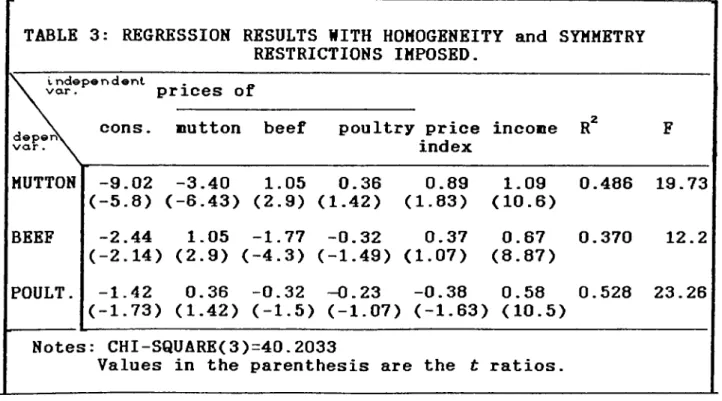
4.4.3 Model 3: Homogeneity and Symmetry Restrictions Imposed After testing for homogeneity and symmetry restrictions
individually, it is possible to test both restrictions
simultaneously. The estimates of the coefficients of the model is given in Table 3.
When the signs of the coefficients are analyzed, it can be seen that in mutton equation, all of the coefficients have the correct signs. In beef equation the coefficient of poultry price
is negative. In poultry equation only the mutton price and
income coefficients have the correct signs.
When the individual significances of each coefficient, are
analyzed, it can be seen that in mutton and beef equations all of the coefficients except that of price index and price of poultry are significant. In poultry equation only income coefficient is significant.
If the joint significance of the coefficients are to be
analyzed, it can be seen that in equations the computed F ratios
O .0 5
are greater than the critical ^^ ^^^-2.17 . Therefore, all
equations are wholly significant at 5Z level of significance.
On the other hand, the test statistic for the restrictions 2
is X^=40.2 which is greater than the critical value. O Therefore,
the homogeneity and symmetry restrictions are rejected, implying
that there may be other factors other than utility maximization for the explanation of the aggregate demand.
When the significance of the price index coefficient
is analyzed, it can be seen that it is not significantly different from zero at 5% level of significance in all of the equations.The percentage changes in income and price index coefficients tend to move together.This may lead to possible multicollinearity problems. In order to avoid this problem, the model is reestimated without the price index variable. The regression results of the model is given in Table 4.
TABLE 3: REGRESSION RESULTS WITH HOMOGENEITY and SYMMETRY RESTRICTIONS IMPOSED. I n d e p e n d e n t . _ v a r . prices of depervy v a r . MUTTON BEEF POULT.
cons. Button beef poultry price
index incone r" F -9.02 -3.40 1.05 0.36 0.89 1.09 0.486 19.73 (-5.8) (-6.43) (2.9) (1.42) (1.83) (10.6) -2.44 1.05 -1.77 -0.32 0.37 0.67 0.370 12.2 (-2.14) (2.9) (-4.3) (-1.49) (1.07) (8.87) -1.42 0.36 -0.32 -0.23 -0.38 0.58 0.528 23.26 (-1.73) (1.42) (-1.5) (-1.07) (-1.63) (10.5) Notes: CHI-SQUARE(3)=40.2033
Values in the parenthesis are the t ratios.
TABLE 4: REGRESSION RESULTS WITH HOMOGENEITY and SYMMETRY RESTRICTIONS IMPOSED and PRICE INDEX VARIABLE DROPPED. \ i n d e p e n d e n t
\ v a r . prices of
d e p e r \ v a r . \
cons. Button beef poultry income r" F
MUTTON -8.57 (-4.83) -5.56 (-6.56) 3.37 (4.39) 1.26 (2.22) 1.039 (9.63) 0.51 26.97 BEEF -3.99 (-3.22) 0.061 (0.104) ( -1.157 -2.15) 0.64 (1.63) 0.697 (9.20) 0.43 19.3 POULT. -1.39 (-1.49) -0.841 (-1.89) 0.38 (0.94) -0.19 (-0.64) 0.607 (10.74) 0.539 29.46 Notes CHI-SQUARE(6)=49.50
Values in the parenthesis are the t ratios •
If the regression results are analyzed, it can be seen that
in nutton and beef equations all of the coefficients are
significant and they all have the correct signs. In poultry
equation only the coefficients of income and mutton price are
significant.
In order to test for the joint significance of the
coefficients, the respective F are computed, shown in Table 4, and 0 . 0 5
compared with the the critical value of F =2.17, it cein be seen
that , they are greater than the critical value. Therefore all of the equations are significant.
When the restrictions are tested,it can be seen that since 2
the computed X^=49.5 is greater than the critical value, the
restrictions are rejected.
When the data of consumptions of mutton, poultry and beef are analyzed,it can be seen that until 1985 the consumption levels are
somewhat stationary. However, in 1985 there is a peak in the
consumption levels in most of the provinces. This may be due to
changes in consumption behaviours. Until early 1980s, mutton and
beef are consumed in general. Poultry is consumed in rural areas.
But in early 1980s , packed chickens introduced to the market and
poultry consumption increased. Therefore, a structural change is
expected between these two periods. In order to test for the
structural change, Chow Test is utilised.Two regressions are run, one for the time period 1979-1984; the other for the time period
1985-1989.These are the unrestricted regressions. The restricted
regression is run for the time period 1979-1989.
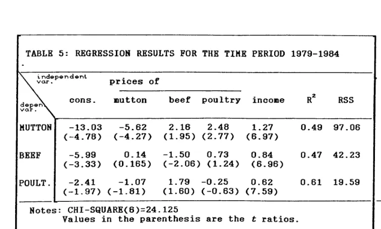
The coefficient estimates of the regression equation for the
first tine period is given in Table 5. As it can be seen fron the table all of the coefficients of the sutton and beef equations have the correct signs. In nutton equation all of the coefficients
are significant. In beef equation only the coefficients of nutton
and beef price are not significant.In poultry equation, the
nutton price coefficient is negative indicating a conplenentarity between nutton and poultry.
When the restrictions are tested, it can be see that both restrictions are rejected at 10% level of significance. The
2 2
conputed o =24.125 is snaller than the critical X =22.45.<5
The coefficient estinates of the regression equations for the tine period 1985-1989 are given in Table 6. As it can be seen
fron the table only the coefficient of poultry price has the
wrong sign and it is the only insignificant coefficient in nutton equation. In beef equation all of the coefficients have the
correct signs. Only the coefficient of incone is significantly
different fron zero. In poultry equation, the coefficient of
nutton price is negative and only the incone coefficient is significant.
When the restrictions are tested, it can be seen that the
2 2
conputed X^=49.46 which is greater than the critical X^=22.45
inplying that the restrictions are rejected.
The restricted regression estinates of the Chow Test are given in Table 4 and explained in section 4.3.3.
TABLE 5: REGRESSION RESULTS FOR THE TIME PERIOD 1979-1984 \ independent
\ var. prices of
deper\ var. X
cons. mutton beef poultry income r" RSS
MUTTON -13.03 (-4.78) -5.62 (-4.27) 2.16 (1.95) 2.48 (2.77) 1.27 (6.97) 0.49 97.06 BEEF -5.99 (-3.33) 0.14 (0.165) -1.50 (-2.06) 0.73 (1.24) 0.84 (6.96) 0.47 42.23 POULT. -2.41 (-1.97) -1.07 (-1.81) 1.79 (1.60) -0.25 (-0.63) 0.62 (7.59) 0.61 19.59 Notes: CHI-SQUARE(6)=24.125
Values in the parenthesis are the t ratios.
TABLE 6: REGRESSION RESULTS FOR THE TIME PERIOD 1985-1989 \ independent
\ var. prices of
depet\ var. \
cons. mutton beef poultry income K RSS
MUTTON - 3 .8 8 - 5 .9 7 5.21 - 0 .1 7 0.803 0.61 50.13 ( - 1 .6 8 ) ( - 5 .7 7 ) (5.28) ( - 0 .2 4 ) ( 6 .4 7 ) BEEF - 3 .9 2 0.183 -0.714 -0 .4 6 5 0.556 0.429 29.99 ( - 2 .2 0 ) (0 .2 2 9 ) ( - 0 .9 3 ) ( - 0 .8 5 ) ( 5 .7 9 ) POULT. - 1 .1 0 - 0 .2 9 0.08 -0 .3 1 4 0.54 0.49 21.69 ( - 0 .7 2 ) ( - 0 .4 2 ) (0 .1 2 ) ( - 0 .6 8 ) (6 .7 1 ) Notest: CHI-SQUARE(6)=49. 46
Values in the parenthesis are the t ratios.
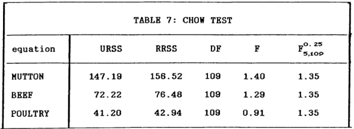
The Chow Tests for each equation are perforned in Table 7.As it can be seen fron the table, the conputed F ratio of the nutton
0^5
equation exceeds the critical value is F =1.35. Therefore, it
5,10^
can be seen that there is a structural chaunge between these two
periods in mutton equation. However, the computed F ratios of
poultry and beef equations are smaller than the critical F ratio implying that there is no structural change for the beef and poultry equations.
TABLE 7: CHOW TEST
equation URSS RRSS DF F ^5,10i>O. 25
MUTTON 147.19 156.52 109 1.40 1.35
BEEF 72.22 76.48 109 1.29 1.35
POULTRY 41.20 42.94 109 0.91 1.35
4.CONCLUSION
This study investigates the structure of the Turkish Meat Demand and tests for any structural change between the periods (1979-1984) and (1985-1989) due to changes in consumer behaviuor.
In the first part of the study, three demand functions are estimated for the meat items mutton, beef and poultry. Since the classical demand theory requires any demand function to satisfy the homogeneity and symmetry restrictions, they are imposed in the demand equations. In the first model, only the homogeneity
restriction is imposed and tested. But, it is found that the
demand equations do not satisfy the homogeneity restriction. In
the second model, only symmetry restriction is imposed and tested
it is found that the symmetry restriction is accepted. That is
the demand functions satisfy the symmetry restriction. In the
third model, both of the restrictions are imposed together.
However, the demand functions failed to satisfy both of the
restrictions.
In each model individual and joint significances and the
signs of the coefficients are examined.lt is found that, the
coefficient of the price index variable in each equation is insignificant. Furthermore the inclusion of the income and price index variables together may lead to some multicollinearity
problems. Therefore, the price index variable is excluded and
the model is reestimated with symmetry and homogeneity
restrictions imposed.