Anomaly detection in time series

KADİR HAS UNIVERSITY SCHOOL OF GRADUATE STUDIES PROGRAM OF COMPUTER ENGINEERING

ANOMALY DETECTION IN TIME SERIES

TAHA A. AL-BAYATI

MASTER’S THESIS

Ta ha A. A l-B aya ti M.S The sis 20 19 S tudent’ s F ull Na me P h.D. (or M.S . or M.A .) The sis 20 11

ANOMALY DETECTION IN TIME SERIES

Taha A. Al-Bayati

MASTER’S THESIS

Submitted to the School of Graduate Studies of Kadir Has University in partial fulfillment of the requirements for the degree of Master’s in the Program of

Computer Engineering

ii

TABLE OF CONTENTS

3.1 Support Vector Machine ... 17

3.2 Decision Tree ... 21

3.3 Autoencoder ... 26

4.CONCLUSIONS ... 32

REFERENCES ... 33

i

ANOMALY DETECTION IN TIME SERIES

ABSTRACT

The concept of “Internet of Things” is based on connecting any physical object through the internet. This will facilitate our daily lives by dedicating technology in our will. In such a world, the number other interconnected devices is enormous, hence, the need for high performance processing in real-time is huge. This research shines light on the importance of the event processing and machine learning in the time series. A multiple of machine learning algorithms such as support vector machine, decision tree, autoencoder, and K-mean clustering are used for training a time series. A comparison of different methods is analyzed to obtain a robust conclusion about the data. The time series data is used to distinguish the state of emotions for a group of people (15 in total) who participated in an experiment. The state of the emotion may be in one of the four states: stressed, amused, natural, and sad. In this work, we compared the performance of algorithms in terms of their accuracy of predicting the emotions.

ii

ZAMAN SERİLERİNDE ANORMALLİK YAKALANMASI

ÖZET

Nesnelerin interneti kavramı herhangi bir fiziksel nesneyi internete bağlamaya dayanır. Bu, teknolojiyi isteklerimiz yönünde kullanmaya sevk ederek günlük hayatımızı etkileyecektir. Böylesi bir dünyada birbirine bağlı cihazların sayısı muazzam olacak ve gerçek zamanda yüksek performanslı very işlemeye ihtiyaç duyulacaktır. Bu araştırma, zaman serilerinde olay işleme ve makine öğrenmesinin önemi konusuna ışık tutmaktadır. Bir zaman serisinin eğitimi için farklı makine öğrenmesi algoritmaları kullanılmıştır: destek vektör makinesi, karar ağaçları, otokodlayıcı ve K-ortalama öbekleyici. Veri hakkında sağlam bir sonuca varmak için farklı yöntemlerin kıyaslaması yapılmıştır. Bu zaman serisi verisi 15 kişilik bir grubun duygu durumunu ayırt etmeye yarayan ölçümlere dayanmaktadır. Bunlar şu dört durumdan biridir: stresli, eğlenmiş, doğal, üzgün. Bu çalışmada duyguların öngörülmesindeki doğruluk cinsinden algoritmaların performansları karşılaştırılmıştır.

Anahtar Sözcükler: Nesnelerin interneti, sağlık hizmetleri, anormallik yakalama, makine öğrenmesi

iii

ACKNOWLEDGEMENTS

I would like to express my thanks and gratitude to my supervisor Asst. Prof. Dr. Arif Selçuk ÖĞRENCİ for his guidance and for stimulating me with energy in my hardest times. Also, for encouraging to pursuit my goal when I wanted to give up.

iv

To my parents Thank you for supporting me through this journey emotionally by tracing my progress and reminding me of my goals in life, My dear mother and father I’m apricated for the faith you have in me during my ups and downs and always believe in me even when I didn’t believe in myself and supporting me financially. My beloved sisters I’m grateful for guiding me in my currier and helping me to reach this goal by cheering me and your advice was always what I needed. Also my aunties for looking after me and my family. To my loyal friends Mohammed Noori, Mohammed Ismail, Ali Bora and Tahsin Tabba, who taught me the from their knowledge and invited their time on guiding me to the last minute. And in the end, I want to thank my friends Haider Al-Faiad, Yousif Al-Faiad, Ammar Dhuwaib, Waleed Alzubaidi and Hassan Jumaily who supported my decision and cheered me up .

v

LIST OF TABLES

Table 2.1 The training dataset ………...13

Table 2.2 The test dataset ………..….….14

Table 3.1 Confusion matrix: accuracy for SVM…….………...……...…19

Table 3.2 Confusion matrix: accuracy for Dtree………..………....22

Table 3.3 Confusion matrix: accuracy for Autoencoder ………...27

vi

LIST OF FIGURES

Figure 1.1 Big Data Source in IoT ………...……….……....2

Figure 1.2 A high-level system model of IoT ……….……….3

Figure 2.1 Wrist wearable device ……….………...………..12

Figure 2.2 RespiBAN biological device ……….……….……….14

Figure 2.3 Data gathering structure ………...………...14

Figure 2.4 The representation of the Confusion matrix ……….…….………..……….16

Figure 3.1 The dialog box to select the algorithm to be used …...………...………17

Figure 3.2 The position of the original points in the SVM algorithm ……….19

Figure 3.3 The position of the training points in the SVM algorithm …...…..…...20

Figure 3.4 The location of the emotion’s classes ……...………...……….…....21

Figure 3.5 The position of the training points in the decision tree algorithm…...….23

Figure 3.6 The location of the emotions classes ……….……….………...……….……..24

Figure 3.7 The decision tree that was used for classifying the data ………….…………25

Figure 3.8 The decision tree after applying the pruning ..………...……….….…….26

Figure 3.9 The location of the training points of the emotions………...……….……28

Figure 3.10 The regions of the emotions ………...………..29

vii

LIST OF SYMBOLS

ACC Three-axis acceleration

BLE Bluetooth low energy

BVP Blood Volume Pulse

DoS Server attack

Dtree Decision tree

ECG Electrocardiogram

EDA Electrodermal activity

EMG Electrocardiogram

IoT Internet of Things

IP Internet protocol

IPV4 Internet protocol version 4

IPV6 Internet protocol version 6

M2M Machine to Machine

NCTA The National Cable &Telecommunications Association

SVM Support-vector machine

1

1. INTRODUCTION

This chapter will give fundamental information for Internet of Things and the biological sensors employed to collect the data which are used for anomaly detection by means of machine learning algorithms. The chapter presents the motivation and defines the aims of this research work. Further, the thesis contributions are highlighted.

1.1 Problem statement

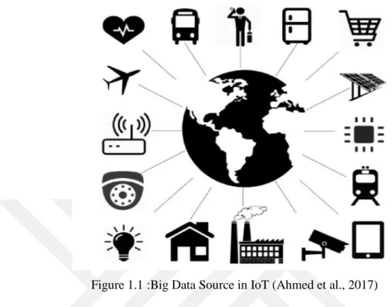
Internet of things (IoT) stands for any physical device connected to the internet to make the life of the humans easier and practical (Ahmed et al., 2017). IoT is a system for exchanging and computing the information between the devices via the network without the interaction of the human beings (Ahmed et al., 2017). Everyday life objects will be equipped with microcontrollers, transceivers and receivers for digital communication. Appropriate sets of protocols are developed that will enable those components to communicate with each other and with users, becoming an integral part of the Internet, as illustrated in Figure 1.1. The ultimate aim of IoT is to facilitate human life intelligently without human intervention. IoT systems will form a modern form of communication that is envisioned in the near future (Madakam et al., 2015). There are different applications in the field of IoT such as in the industrial sector, health care, military and vehicular systems and it expected to involve every part of human life. The technology is growing every day and the human innovation and need is shifting us to the IoT era, these are driving forces and concept ideas that are aligned with the IoT system and it will lead the way for the new generation. As the number of interconnected devises increase, many challenges arise exponentialy with it such as the need to carry out the necessary computations (Rghioui and Oumnad, 2017).

2

Figure 1.1 :Big Data Source in IoT (Ahmed et al., 2017)

The computations form a very intricate issue in terms of processing the information. The time is a critical feature in the edge devices and even small delays can sometimes lead to a catastrophic incident (Kong et al., 2017).

In Big Data generation the amount of the information generated is huge and this data is sent in a short amount of time to the cloud to be processed and stored. However, this amount of data sometimes can over load the cloud with meaningless information and the cost of processing increases. The storage of the data is also a problem and it is impossible to save every little detail due to the enormous size of the information (Ang et al., 2017).

Another similar issue arises with the Big Data, which is the network cost. Just as the processing cost of the information increases, the network load is exponentially increasing with the amount of data sent to the cloud. This data also leads to a load on the network while the data propagate from the edge device to the cloud. The result will be increases in the delay of exchanging the information and a late response caused by the congestion and shows the inefficiency of the system (Cao et al., 2016).

In such enormous data flow collected from different resources such as smart house, smart gadgets, autonomous vehicles and smart cities, data loss is another factor leading

3

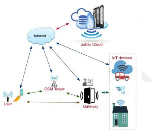
to miss communicating and allowing the data (Zanella et al., 2014 ) to be compromised to attacks such as the denial of server attack (DoS). Hackers exhibit a major threat to cloud servers which seek to get the information of users and these attacks accrue in a short period of time. In such attacks, the verification of the information is set to the end user (Ammar et al., 2018). These vulnerabilities have raised the bar for traditional algorithms of detecting fraud and Figure 1.2 illustrates the need of complexity in the IoT network system.

Figure 1.2: A high-level system model of IoT (Ammar et al., 2018)

In spite of the problems of the system there are many driving forces leading us to the expunction of the IoT era. Every technology, which develops daily in every field, helps to create a wide network of information (Al-Fuqaha et al., 2015). Sensors generate this data or devices are variable due to the increase of the interconnected sensors to the network. In every day the price of the semiconductors, transistors are getting smaller and cheaper which is one of the most import drivers of the IoT era. The future of the technology mainly relies on sensors. The sensors are the means of extracting data and

4

interconnected sensors to the network are everywhere thanks to the small cost of it, which takes us one-step closer to the IoT era.

The more interconnected devices increase, the need of IP's exponentially increase with it. As explained before, each device or sensor connected to the internet is connected using an IP (Internet protocol) address. The new protocol IPV6 (Internet protocol version 6) offers specific IP addresses to every device that is used across the network providing it with almost infinite numbers of IPs. This is not the case in IPV4 (Internet protocol version 4) which is confronting a problem of inefficient IP addresses by providing approximately 4.3 billion. The IPV6 addresses are enough to satisfy the need of the devices in the concept idea of the IoT systems (“IPv6 Addressing and Basic Connectivity Configuration Guide, Cisco IOS XE Release 3S - IPv6 Addressing and Basic Connectivity”). Such capable tools will allow the integration of IoT and 5G platform (Ali et al., 2015). The inspiration of this work is based on these issues and the driving forces of this field and the need of improving the anomaly detection field that is responsible to handle these issues.

5 1.2 Objective

The objective behind this thesis is to develop an algorithm that is capable to handle real-time data in order to detect the outliers in the data. This algorithm is meant to compere two time series that if there are N time series for the same quantity taken at different time intervals. This interval is meant to be applied in real-time data generated by using MATLAB (Lara et al., 2008), which is a suitable programing language that can handle outlier detection. The algorithms are applied for a number of times in order to obtain satisfying results. The algorithm is supposed to be operating in real-time for the dataset and it’s a conception idea for an IoT platform which requires a high speed response and detecting for anomalies simultaneously preserving a low error rate and a low false positive sample ratio. The other objective of the algorithm is to determine the pattern on the data series by applying a mathematical equation in order to make comparisons between data series and to understand the data. The context of the data is recognized by the model and based on it, context aware models can be combined with it (Rahman et al., 2017). Real time data series form the most controversial topic in today's technology due to the massive M2M (Machine to Machine) interactivity. New challenges appear in many fields of M2M communication such as security, processing performance and network delay (Kim et al., 2014).

1.3 Literature

The advances in the electronics technology of the IoT world has increased the number of interconnected devices such as smart sensors. These sensors collect information and share it in the cloud service to be processed. The National Cable &Telecommunications Association (NCTA) showed a study that elucidate to the number of interconnected devices which is about 50.1 billion IoT devices in the year of 2020 (El-Sayed et al., 2018).

The system has to sustain a certain degree of standardization so it holds suitable for a wide range of applications within various industry sectors such as health, cars, smart phones, or smart cities. Hence, the IoT technology has to evolve based on open

6

standards. In other words, innovation thrives on open standards that facilitate interoperability while retaining a degree of functional standardization (Peine, 2009, pp. 406). This requires both a certain degree of looseness as a certain degree of rigidness of the system. This area is still lacking of full understanding in these days (Atzori et al., 2010; Fell, 2014; EP, 2015). Therefore, this research tries to fill this need of providing visions in how this issue has been handled in the past and which lessons should be learned from that. For example, how can increases in storage happen without the presence of a dominant design? Which implications have open standards for product and process innovation? What kind of dominant design can exist together with open standards? Which innovation strategy should a company ideally implement in order to manage innovation based upon open standardization?

This research finds its societal relevance in providing insights for many different players in the field of IoT. Understanding the nature of IoT is a key element towards devising adequate policy measures for its creation and diffusion. Because no ‘traditional’ dominant design emerges, policy makers need to make choices based on open standards. This research provides insights in these open standards and thus serves as a guideline for policy makers in the field of IoT. There are several major challenges that impact a broad implementation of IoT. First, as mentioned earlier, IoT is a complex structure of hardware, sensors, applications and devices that need to be able to communicate between different geographical locations. Second, ownership of data is and probably will remain a difficult topic for years, but it is probably shifting to having access to the data and being able to use it for analysis. Moreover, mixing the digital and the physical world will require high security standards in order to prevent accidents (Atzori et al., 2010; Fell, 2014). Furthermore, standards can provide cost efficient realizations of solutions (IERC, 2015).

In the stocks the value of the market changes frequently in very high rate according to the effectiveness of the environment and the factors that affect it in this order outlier detection algorithms are applied to obtain information about the stocks to predict early changes in the market (Chandola et al., 2009). Another field that anomaly detection is applied on is health systems that absorb the information of the end user in order to evaluate the patient health condition and be able to response quickly to sudden anomalies and determines certain patterns that evaluate the state of each patient

7

(Nakamura et al., 2016). Global standards are needed to achieve economy of scale and interworking. In order to deal with these challenges, a comprehensive understanding of how IoT develops and what elements help to set standards will be very useful. This research will contribute to this understanding. Many algorithms are applied in the field by many scientists racing to get robust results such as adaptive greedy model based on norm constraint. The method is applied by allocating the database into a train and test samples and then applying unsupervised learning algorithms to validate the system having the most satisfying results and for optimizing the problem an adaptive forward backward algorithm is used (Hou et al., 2019). A novel method has been applied on a certain model to obtain a high accuracy results in about 95% and the low caution is 5% but this value is affected due to external condition and it might be unsuitable to obtain a correct result in the process. Adapting the environmental circumstances for the algorithm is a highly critical factor to the performance of anomaly detection and it might reattach it from its own purpose (Vengatesan et al., 2018). IoT technology is also used in the health sector for helping patents with Parkinson disease by establishing a edge-fog-cloud network that runs in real time processing information collected from sensors attached to the patient. The model runs on the idea of distributed processing between all the IoT layers in order to ensure the highest data rate and less processing power. BLE (Bluetooth low energy) technology also depends on real-time processing. BLE is used in almost every book shop around the world due to its light weight and cheap price. BLE has been found very practical. A system has been developed by using BLE to track the movement of elderly people for their need and the system runs for indoor environments and each beacon is attached to an elderly and their movement tracked down in order to alarm for any unusual activity. The data gained from the BLE beacon runs through an edge device with limited capabilities and a lightweight algorithm (Cay et al., 2017; Jeon et al., 2018). Real-time processing is commonly used by the node platform that collects the information from sensors, social media and cellphones (Islam et al., 2015).

8 1.4 IoT in Healthcare

Healthcare services is a very important and vastly growing sector. The need for better service in this field is highly demanded. Due to the lack of highly efficient service and excellent labor, there is an open opportunity to the research world to step up and provide an alternative. In some cases, the need for those who are excellent in this field need to be recorded, with today’s technology certain applications, or apps, can be designed to replace them or give a sample diagnosis. Such apps give simple questions to identify the disease and give guidance to the treatment or primary's consultant whether it should or should not see a doctor. IoT can assist to find some answers to many problems in this field where it can offer fast medical help, and step by step tutorial for certain cases where the personal mobile can replace a home nurse and be absorptive of the patient in some cases (Islam et al., 2015).

9

2. Methodology of Research

The basic step in the methodology is data processing. As anomaly detection can be regarded as a machine learning task with big data, the data set becomes of utmost importance. The journey of our work starts from the dataset.

Firstly, we extracted the dataset from the raw data, then, we started preprocessing the data by normalizing it using norms so that they can be used in machine learning algorithms which is converting it to a number between 0 to 1. Then we started applying cleaning algorithms; the dataset has to be processed to identify missing data and perform interpolation if this is necessary. In case the interpolation is not feasible because the amount of missing data is large in the single record, the data will be discarded. Next, data will be sampled to remove repeating sets of data which would not give valuable information as the repeating data may also cause a bias in learning. Last but not least, data can be extended by deriving some new sets of attributes based on available ones, hence features can be derived for the data. The important point is to be careful about including pieces of data that are relevant for the objective of anomaly detection.

In this research an outlier detecting algorithm is proposed to evaluate the multi-dimensional time series. The dataset is gathered that is already applied by a different model in the same purpose of detecting anomalies. MATLAB programming will be used in this research to the mentioned database the first step is preprocessing the data and prepare the data for the machine learning algorithms by applying feature selection that evaluate the features and ignore the features that reduce the quality of the output results then we apply a feature method that fills or ignore the missing column due to the algorithm’s functionality (Schmidt et al., 2018). These datasets are generated with the same values but with a random distribution, which represent the different interval between the dataset. After the generation of the data a supervised SVM (Support-vector machine) algorithm is applied to the dataset to figure out the trends and the anomalies of it, then the same algorithm is applied in different intervals. Moreover, another datamining algorithm is applied to the data series which is SVM. In this order the

10

accuracy of the result should increase and the efficiency of the processing is kept adequately.

Another approach to be employed is to combine outputs of several supervised and unsupervised methods to form a decision. As the data are labeled, that is, desired outputs for categories are known, supervised methods such as neural networks and decision trees can be employed. On the other hand, also unsupervised clustering and autoencoder networks can be used. Clustering for different cluster counts will be performed and each cluster will be checked for their composition. If a cluster includes, say more than 90 percent of a certain category, then clustering can be used to support the decision-making process for that category. On the other hand, the autoencoder network can also be used to check the error level for each input pattern. The network is trained to learn the given inputs as the desired outputs, and if a certain input exhibits an error level considerably larger than the average (for experimental purposes this may be set to a given percentage) this sample is considered as an anomaly.

2.1 Dataset

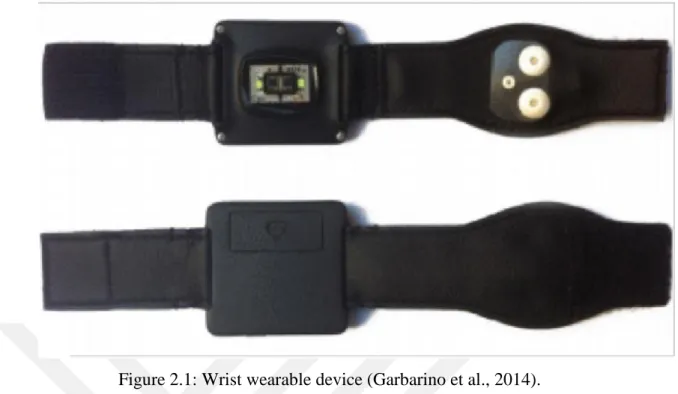
The database is gathered using wearable devices attached to the human body in order to detect the emotions. By the activities the person carries out, the mood of the person will be predicted as one of the four classes: stress, amusement, sad or natural. Human-computer interaction has always been a mystery but with today's technology this mystery is unravelling. The data was collected from 17 participants where results for two individuals (S1 and S12) were discarded due to malfunctioning of sensors thus giving unreliable results. The data is measured through biological sensors, which are RespiBAN and Empatica E4. The Empatica E4 device is capable of extracting information by attaching it to the wrist and the chest and then transforming this data to be analyzed as shown in Figure 2.1.

11

Figure 2.1: Wrist wearable device (Garbarino et al., 2014).

The data collected from RespiBAN wearable are electrocardiogram (ECG), electrodermal activity (EDA), electrocardiogram (EMG), respiration, temperature, and the acceleration in three-axis and it's measured with a frequency of 700 Hz (Wearable Stress and Affect Detection). Meanwhile the data which is gathered from the Empatica E4 is blood volume pulse (BVP, 64 Hz), electrodermal activity (EDA, 4 Hz), body T (temperature) (4 Hz), and ACC (three-axis acceleration) (32 Hz). In audio compiling, the Mel-frequency cepstrum is a portrayal of the little portion of the power spectrum of an audio, constructed by the linear cosine transform of a log power spectrum on a nonlinear Mel scale of frequency. Mel-frequency cepstral (MFC) coefficients are coefficients that jointly build up an MFC, so we used two frequencies which are Mfcc60 and Mfcc99 after normalizing them.

The number of instances found in this database is 4000 samples which was cleaned and chosen in roughly even between classes that are (stressed, amused, natural, sad) from a 1 million dataset, then we divide the data into training and test samples, we used a random function that divides the data in two datasets and the ratio of the division is 70% of the data is set for the training with 2800 samples and the other 30% is set for the test with 1200 using the following code:

12 [m,n] = size(TrainingSet) ; P = 0.70 ; idx = randperm(m) ; Training = TrainingSet(idx(1:round(P*m)),:) ; Testing = TrainingSet(idx(round(P*m)+1:end),:) ;

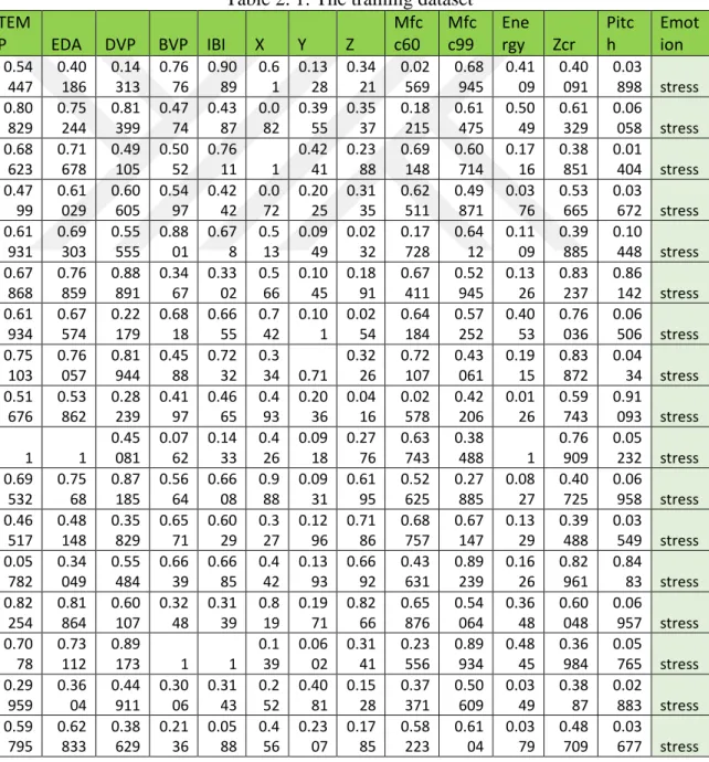
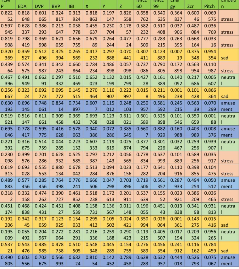
Both data sets are meant to be classified but the training part used to extract the information meanwhile the test dataset is used to evaluate the accuracy of the system. Table 2.1 shows a snapshot of the training data set meanwhile Table 2.2 is a portion of the test dataset.

Table 2. 1: The training dataset TEM P EDA DVP BVP IBI X Y Z Mfc c60 Mfc c99 Ene rgy Zcr Pitc h Emot ion 0.54 447 0.40 186 0.14 313 0.76 76 0.90 89 0.6 1 0.13 28 0.34 21 0.02 569 0.68 945 0.41 09 0.40 091 0.03 898 stress 0.80 829 0.75 244 0.81 399 0.47 74 0.43 87 0.0 82 0.39 55 0.35 37 0.18 215 0.61 475 0.50 49 0.61 329 0.06 058 stress 0.68 623 0.71 678 0.49 105 0.50 52 0.76 11 1 0.42 41 0.23 88 0.69 148 0.60 714 0.17 16 0.38 851 0.01 404 stress 0.47 99 0.61 029 0.60 605 0.54 97 0.42 42 0.0 72 0.20 25 0.31 35 0.62 511 0.49 871 0.03 76 0.53 665 0.03 672 stress 0.61 931 0.69 303 0.55 555 0.88 01 0.67 8 0.5 13 0.09 49 0.02 32 0.17 728 0.64 12 0.11 09 0.39 885 0.10 448 stress 0.67 868 0.76 859 0.88 891 0.34 67 0.33 02 0.5 66 0.10 45 0.18 91 0.67 411 0.52 945 0.13 26 0.83 237 0.86 142 stress 0.61 934 0.67 574 0.22 179 0.68 18 0.66 55 0.7 42 0.10 1 0.02 54 0.64 184 0.57 252 0.40 53 0.76 036 0.06 506 stress 0.75 103 0.76 057 0.81 944 0.45 88 0.72 32 0.3 34 0.71 0.32 26 0.72 107 0.43 061 0.19 15 0.83 872 0.04 34 stress 0.51 676 0.53 862 0.28 239 0.41 97 0.46 65 0.4 93 0.20 36 0.04 16 0.02 578 0.42 206 0.01 26 0.59 743 0.91 093 stress 1 1 0.45 081 0.07 62 0.14 33 0.4 26 0.09 18 0.27 76 0.63 743 0.38 488 1 0.76 909 0.05 232 stress 0.69 532 0.75 68 0.87 185 0.56 64 0.66 08 0.9 88 0.09 31 0.61 95 0.52 625 0.27 885 0.08 27 0.40 725 0.06 958 stress 0.46 517 0.48 148 0.35 829 0.65 71 0.60 29 0.3 27 0.12 96 0.71 86 0.68 757 0.67 147 0.13 29 0.39 488 0.03 549 stress 0.05 782 0.34 049 0.55 484 0.66 39 0.66 85 0.4 42 0.13 93 0.66 92 0.43 631 0.89 239 0.16 26 0.82 961 0.84 83 stress 0.82 254 0.81 864 0.60 107 0.32 48 0.31 39 0.8 19 0.19 71 0.82 66 0.65 876 0.54 064 0.36 48 0.60 048 0.06 957 stress 0.70 78 0.73 112 0.89 173 1 1 0.1 39 0.06 02 0.31 41 0.23 556 0.89 934 0.48 45 0.36 984 0.05 765 stress 0.29 959 0.36 04 0.44 911 0.30 06 0.31 43 0.2 52 0.40 81 0.15 28 0.37 371 0.50 609 0.03 49 0.38 87 0.02 883 stress 0.59 795 0.62 833 0.38 629 0.21 36 0.05 88 0.4 56 0.23 07 0.17 85 0.58 223 0.61 04 0.03 79 0.48 709 0.03 677 stress

13

Table 2. 2: The test dataset TEM P EDA DVP BVP IBI X Y Z Mfcc 60 Mfcc 99 Ener gy Zcr Pitch Emotio n 0.822 52 0.818 648 0.601 065 0.324 817 0.313 924 0.818 863 0.197 147 0.826 558 0.658 762 0.540 635 0.364 837 0.600 46 0.069 575 stress 0.597 945 0.628 337 0.386 293 0.213 647 0.058 778 0.455 637 0.230 704 0.178 57 0.582 232 0.610 408 0.037 906 0.487 084 0.036 769 stress 0.819 908 0.798 419 0.369 998 0.621 055 0.656 755 0.679 89 0.264 244 0.477 24 0.777 509 0.283 215 0.263 395 0.668 164 0.033 16 stress 0.320 369 0.359 527 0.512 496 0.325 394 0.265 569 0.417 232 0.297 888 0.070 441 0.307 411 0.123 889 0.007 19 0.375 348 0.954 354 sad 0.439 64 0.574 575 0.341 987 0.342 243 0.660 864 0.784 234 0.486 898 0.057 098 0.737 086 0.790 805 0.172 898 0.563 954 0.110 987 stress 0.467 396 0.491 949 0.662 91 0.297 332 0.510 469 0.652 023 0.132 199 0.015 799 0.427 28 0.161 389 0.140 092 0.217 686 0.005 607 neutra l 0.256 667 0.323 24 0.092 773 0.095 772 0.145 515 0.270 464 0.116 907 0.222 997 0.015 8 0.211 496 0.001 238 0.101 428 0.866 364 sad 0.630 193 0.696 145 0.748 061 0.854 14 0.734 897 0.607 7 0.115 012 0.248 103 0.250 957 0.581 592 0.245 215 0.563 39 0.070 299 amuse ment 0.519 921 0.516 147 0.611 661 0.309 458 0.369 432 0.693 768 0.123 028 0.611 021 0.601 589 0.525 898 0.101 546 0.350 659 0.001 88 neutra l 0.695 046 0.778 417 0.595 775 0.416 628 0.578 063 0.940 386 0.072 286 0.385 545 0.660 7 0.882 929 0.160 988 0.403 989 0.008 376 amuse ment 0.221 392 0.316 675 0.514 759 0.044 285 0.223 152 0.607 333 0.119 619 0.025 874 0.377 794 0.301 226 0.032 467 0.259 256 0.939 907 neutra l 0.230 098 0.399 576 0.701 286 0.628 932 0.525 585 0.797 387 0.212 143 0.056 565 0.778 834 0.637 993 0.101 889 0.589 256 0.035 917 stress 0.619 313 0.693 028 0.555 553 0.880 134 0.678 042 0.513 284 0.094 876 0.023 156 0.177 282 0.641 204 0.110 916 0.398 855 0.104 475 stress 0.489 883 0.577 456 0.285 456 0.764 498 0.776 241 0.666 506 0.047 298 0.703 896 0.719 506 0.561 357 0.287 933 0.494 254 0.050 512 amuse ment 0.318 2 0.332 158 0.474 262 0.390 727 0.461 852 0.518 238 0.172 613 0.201 911 0.537 639 0.155 52 0.023 921 0.386 209 0.026 465 stress 0.451 174 0.468 838 0.424 431 0.451 27 0.408 539 0.158 731 0.136 567 0.011 148 0.196 055 0.451 43 0.013 838 0.341 98 0.931 813 neutra l 0.192 206 0.342 45 0.317 059 0.123 925 0.154 033 0.295 412 0.105 502 0.024 421 0.350 994 0.026 064 0.001 361 0.143 275 0.015 416 sad 0.195 009 0.055 492 0.204 967 0.272 064 0.281 291 0.216 336 0.259 188 0.290 423 0.119 215 0.405 507 0.017 194 0.209 324 0.956 265 neutra l 0.537 21 0.543 476 0.485 985 0.478 758 0.510 505 0.548 348 0.445 285 0.154 755 0.276 589 0.456 354 0.241 912 0.116 162 0.784 459 sad 0.490 805 0.603 556 0.702 675 0.566 993 0.682 24 0.810 54 0.142 452 0.789 458 0.628 283 0.632 957 0.444 018 0.526 793 0.075 067 amuse ment

14

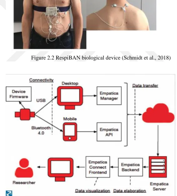
The database is collected through wearable sensors attached to the human body as shown in Figure 2.2. These sensors are connected to the cellphone of the person wearing them and then data are sent to though servers to be analyzed using machine learning algorithms. After the processing the algorithm will make a decision about the state of the human and sends back a feedback to the same cellphone as shown in the Figure 2.3.

Figure 2.2 RespiBAN biological device (Schmidt et al., 2018)

15 2.2 Data mining

Data mining is a mathematical approach of processing large data to determine its modality and its patterns. Data mining techniques first preprocess the data then it will be analyzed and post processed before the visualization step. Data mining can be categorized in two types of algorithms: supervised and unsupervised learning. Data mining is connected with every single aspect of our life (Ming et al., 2018). The algorithms used in this work are support vector machine, decision tree, and autoencoder.

2.2.1 SVM

A Support Vector Machine (SVM) is a distinguishing method of classifying two groups formally defined by a separating hyperplane. In other words, given class training data (supervised learning), the algorithm labels an optimal hyperplane which categorizes all data belonging to either the first or the second group. In two dimensional space, this hyperplane is a line dividing a plane into two parts wherein each class lay in either side. SVM is widely used among face recognition software packages. The advantage of using SVM is that it can find an enormous correlation between data points with applying less complicated operations and transformations which decreases the duration of computations.

2.2.2 Decision Tree

A decision tree is a method of making decisions which uses an algorithm that is assembled as a tree and it produces a bunch of outcomes such as actions or costs. It handles data with class labels and it trains a model according to the entropy of each element in the data set, then it performs a series of one directional operations in order to determine the height accuracy label. Decision tree algorithm can be used for prediction tasks such as:

1. Finance and predicting trends in the stock markets, 2. Weather forecasting,

3. Security and detecting threats, 4. Video surveillance.

16 2.2.3 Autoencoder

Autoencoders are neural networks to analyze the patterns by extracting and comparing the input instances to the output of the operation. The basic idea of autoencoder is to combine an encoder and the decoder. In the encoder part the input of the algorithm is compressed to a latent space representation by the function h=f(x). As for the decoder part it regenerates the input from the latent space representation by the function r=g(h). Since it’s a neural network unsupervised learning method it can be used commonly in noise detection programs.

2.3 Accuracy measurements

The functionality of every system is measured by certain metrics expressed quantitatively that are suitable to the system itself. In our case, we have chosen both F-score and the confusion matrix for accuracy. The F-F-score is a method of finding the test accuracy for the system by weighted harmonic mean. It is measured by calculating the recall and the precision as shown below:

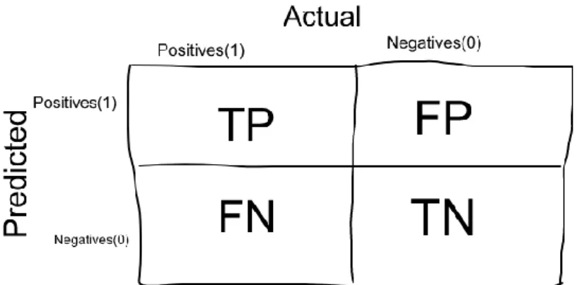
where the precision is defined as the ratio of the “true positives” to the sum of positives, and the recall is the ratio of “true positives” to the sum of true positives and false negatives. Meanwhile in the confusion matrix we construct a table to determine the efficiency of the system and it is often used with class labels with different attributes. The error matrix method gives a full description of the output for the system and it is described as shown in Figure 2.4.

17

3. Results

For the analyses carried out in this thesis, the MATLAB programming environment has been used. Specifically, the built-in libraries of the package are utilized. In MATLAB a dialog box was created to prompt the user to select the machine learning algorithm that will be used to detect the emotions from the dataset. The dialog box is illustrated in Figure 3.1.

Figure 3.1 The dialog box to select the algorithm to be used.

The first two techniques are supervised machine learning whereas the last one is the unsupervised learning and the data is already divided and imported to Matlab.

3.1 Support Vector Machine

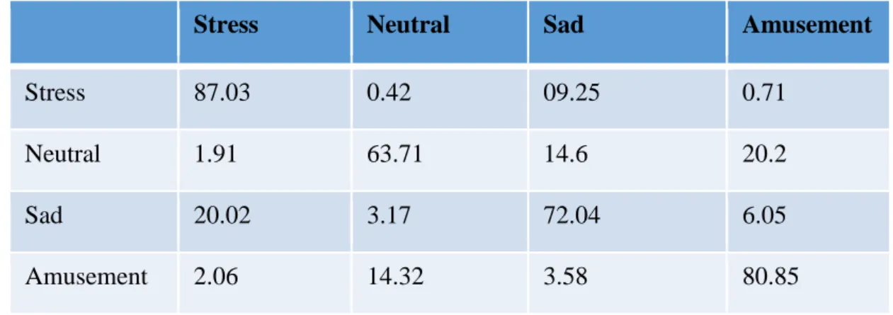
The multi class support vector machine (SVM) was used to classify the four emotions recorded in the datasets. The test accuracy of this algorithm was 74% as eleven of the 15 participants were fully classified. The overall accuracy of the training data was 76% for the SVM algorithm. The confusion matrix was converted to percentage values as shown below in Table 3.1.

18

Table 3. 1: Confusion matrix: accuracy for SVM

Stress Neutral Sad Amusement

Stress 87.03 0.42 09.25 0.71

Neutral 1.91 63.71 14.6 20.2

Sad 20.02 3.17 72.04 6.05

Amusement 2.06 14.32 3.58 80.85

The F score was calculated also as shown below:

19

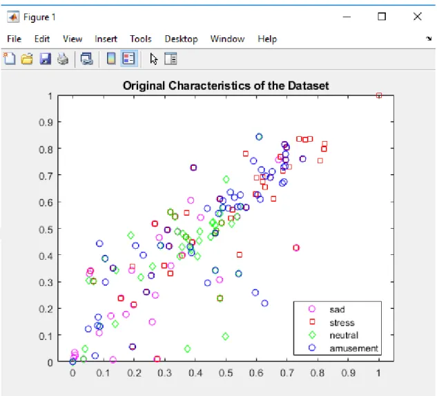
Figure 3. 2:The position of the original points in the SVM algorithm

In Figure 3.2, the locations of the emotion points are plotted as identified in the training data set for the SVM algorithm. When the data points are plotted after the training to represent the participant emotions, we obtain Figure 3.3. The most dominant emotion based on the training and testing in SVM was stress. Neutral and sadness were intertwined and occurred in the same region of the plot.

20

21

Figure 3.4 The location of the emotions classes.

After deploying SVM algorithm to the dataset we can distinguish in Figure 3.4 that the most dominant state of mind was the stress which is denoted by the blue square. The data were separated by the SVM hyperplane for the dataset as shown in Figure 3.3.

3.2 Decision Tree

The decision tree is another form of supervised machine learning that was used to classify the emotions of each participant. The training and testing was completed giving the confusion matrix below in Table 3.2. In the simulation, the training accuracy of decision tree algorithm was 96.8% and the testing accuracy was 95% meaning that the

22

data for 14 participants were accurately classified. The confusion matrix was converted to percentage values that shows the distribution of the data among classes.

Table 3.2: Confusion matrix: accuracy for Dtree

The data above illustrate that the training in decision tree algorithm was closely knit with most points classified as shown in Table 3.2.

The F score was calculated also as shown below:

And the result was 96%.

Stress Neutral Amusement Sad

Stress 95.58 0.56 0.56 0.71

Neutral 2.21 96.9 0.73 0.59

Amusement 1.29 0.72 98.41 0.86

23

Figure 3.5 The position of the training points in the decision tree algorithm.

Figure 3.5 displays the location of the emotions when the points are plotted for the decision tree algorithm. The training data in decision tree illustrate that most of the participants were stressed. Contrary, to the case in SVM, the neutral and amusement overlapped with most participants excluding some instances of sadness but to minimal levels as shown in Figure 3.6.

24

25

Figure 3.7: The decision tree that was used for classifying the data.

Then we used the pruning technique in order to minimize and detect the over fitting that can harm our results, but the result was the same and it was satisfying as shown in Figure 3.7.

26

Figure 3.8: The decision tree after applying the pruning.

In the decision tree algorithm, the cross-validation approach was used to evaluate the training outcome thus this algorithm has a better result compared to the rest of algorithms as shown in Figure 3.8.

3.3 Autoencoder

This is the only unsupervised machine learning algorithm that was used in this research to classify the emotions of the participants. The technique uses backpropagation to set the values for training as captured in the confusion matrix below as shown in Table 3.3. The training and testing accuracy for this technique was over 66%.

27

Table 3.3: Confusion matrix: accuracy for Autoencoder

Amusement Neutral Sad Stress

Amusement 76.34 2.56 17.09 1.99

Neutral 1.76 53.39 15.04 30.23

Sad 19.88 3.31 69.30 8.78

Stress 1.92 14.46 9.36 75.06

Autoencoder is an unsupervised algorithm so the training accuracy equals the test accuracy which leads to

precision = recall in the equation:

And the result for F score will be 66%.

The location of the training points in the graph illustrate that close to half of the participants’ emotions were classified but a significant amount deviated from the training as shown in Figure 3.9.

28

29

Figure 3.10 The regions of the emotions.

The data was plotted to characterize the proportion of each emotion. In the case of the autoencoder algorithm stress was still the most significant emotion but all the other except amusement overlapped in this region as shown in Figure 3.10. The autoencoder algorithm performed dismally therefore a misclassification technique was used to compute the errors in the training data as illustrated in Figure 3.11.

30

Figure 3.11: The error classification of the misclassified points.

The data above illustrate that a substantial amount of nodes were misclassified thus a lower accuracy was attained as shown in Table 3.4 .

Table 3.4 Comparison among performance of the three algorithms. Algorithm Training Accuracy Testing accuracy

SVM 76.21 74.83

Decision Tree 96.86 95.00

Autoencoder 66.67 66.67

We also compared the duration of execution for each algorithm in order to determine the efficiency of each algorithm.

31

Table 3.5: Duration of execution for each algorithm.

Algorithm Duration (Sec)

SVM 18.69

Decision Tree 21.60

Autoencoder 18.75

Although the accuracy of each algorithms is important, when we deal with real time detection the execution time is extremely cost effective to every system. In this work the optimum algorithm was the SVM for providing a satisfying result in an adequate time response as shown in Table 3.5.

32

4. CONCLUSIONS

In this research, we highlighted the need for an efficient anomaly detecting model that can take us one step ahead to the dawn of Internet of things era. The challenges of this evolution is demonstrated and a machine learning algorithm is devised that extracts the anomalies in the data series and compares between them in order to conclude a robust pattern. In this research we aim to apply two machine learning classification algorithms which are decision tree and SVM which are chosen to be suitable for this certain database and capable to extract the pattern and to classify the samples of the object to one of the two categories which are either stress or affection for our data set. The data set, which is meant to be used in this research, is 63,000,000 samples collected by two biological wearable sensors. The proposed method is to randomly choose a certain interval and then apply the first step of deploying the two classification algorithms to figure out the outcomes. In this work we discussed our method and explore the era of internet of thing and big data then we proposed the methods and importance of real time anomaly detection.

33

REFERENCES

Ahmed, E., Yaqoob, I., Hashem, I.A.T., Khan, I., Ahmed, A.I.A., Imran, M., Vasilakos, A.V., (2017). The role of big data analytics in Internet of Things. Computer Networks 129, 459–471.

Al-Fuqaha, A., Guizani, M., Mohammadi, M., Aledhari, M., Ayyash, M., (2015). Internet of Things: A Survey on Enabling Technologies, Protocols, and Applications. IEEE Communications Surveys & Tutorials pp 2347 – 2376.

Ali, A., Hamouda, W., Uysal, M., (2015). Next generation M2M cellular networks: challenges and practical considerations. Networking and Internet Architecture (cs.NI); Information Theory (cs.IT). arXiv

Ang, L.-M., Seng, K.P., Zungeru, A.M., Ijemaru, G.K., (2017). Big Sensor Data Systems for Smart Cities. pp 1259 – 1271 IEEE Internet of Things Journal

Cay, E., Mert, Y., Bahcetepe, A., Akyazi, B.K., Ogrenci, A.S., (2017). Beacons for indoor positioning, in: 2017 International Conference on Engineering and Technology (ICET). pp. 1–5.

Chandola, V., Banerjee, A., Kumar, V., (2009). Anomaly detection: A survey. ACM Computing Surveys 41, 1–58.

Ioannis, Psaras, (2018). Decentralised Edge-Computing and IoT through Distributed Trust. MobiSys ’18, June 10–15, 2018, Munich, Germany.

El-Sayed, H., Sankar, S., Prasad, M., Puthal, D., Gupta, A., Mohanty, M., Lin, C., (2018). Edge of Things: The Big Picture on the Integration of Edge, IoT and the Cloud in a Distributed Computing Environment. IEEE Access pp 1706 – 1717

Garbarino, M., Lai, M., Bender, D., Picard, R.W., Tognetti, S., (2014). Empatica E3 — A wearable wireless multi-sensor device for real-time computerized biofeedback and data acquisition, in: 2014 4th International Conference on Wireless Mobile Communication and Healthcare - Transforming Healthcare Through Innovations in Mobile and Wireless Technologies (MOBIHEALTH). pp. 39–42.

Hou, D., Cong, Y., Sun, G., Liu, J., Xu, X., (2019). Anomaly detection via adaptive greedy model. Neurocomputing 330, 369–379.

IPv6 Addressing and Basic Connectivity Configuration Guide, Cisco IOS XE Release 3S - IPv6 Addressing and Basic Connectivity

34

[https://www.cisco.com/c/en/us/td/docs/ios-xml/ios/ipv6_basic/configuration/xe-3s/ip6b-xe-3s-book/ip6-add-basic-conn-xe.html], n.d. . Cisco.

Islam, S.M.R., Kwak, D., Kabir, M.H., Hossain, M., Kwak, K., (2015). The Internet of Things for Health Care: A Comprehensive Survey. IEEE Access 3, 678–708. Jeon, K.E., She, J., Soonsawad, P., Ng, P.C., (2018). BLE Beacons for Internet of Things

Applications: Survey, Challenges, and Opportunities. IEEE Internet of Things Journal 5, 811–828.

Kim, J., Lee, J., Kim, J., Yun, J., (2014). M2M Service Platforms: Survey, Issues, and Enabling Technologies. IEEE Communications Surveys Tutorials 16, 61–76. Kong, L., Khan, M.K., Wu, F., Chen, G., Zeng, P., (2017). Millimeter-Wave Wireless

Communications for IoT-Cloud Supported Autonomous Vehicles: Overview, design, and Challenges. IEEE Communications Magazine 55, 62–68.

Lara, J.A., Moreno, G., Pérez, A., Valente, J.P., López-Illescas, Á., (2008). Comparing Posturographic Time Series through Events Detection, in: 2008 21st IEEE International Symposium on Computer-Based Medical Systems. Presented at the 2008 21st IEEE International Symposium on Computer-Based Medical Systems, pp. 293–295.

Madakam, S., Ramaswamy, R., Tripathi, S., (2015). Internet of Things (IoT): A Literature Review. Journal of Computer and Communications 03, 164–173.

Ming, J., Zhang, L., Sun, J., Zhang, Y., (2018). Analysis models of technical and economic data of mining enterprises based on big data analysis, in: 2018 IEEE 3rd International Conference on Cloud Computing and Big Data Analysis (ICCCBDA). Presented at the 2018 IEEE 3rd International Conference on Cloud Computing and Big Data Analysis (ICCCBDA), pp. 224–227.

Radanliev, P., Roure, D.D., Cannady, S., Montalvo, R.M., Nicolescu, R., Huth, M., (2018). Economic impact of IoT cyber risk - Analysing past and present to predict the future developments in IoT risk analysis and IoT cyber insurance, in: Living in the Internet of Things: Cybersecurity of the IoT - 2018, pp. 1–9.

Rahman, H., Rahmani, R., Kanter, T., (2017). Multi-Modal Context-Aware reasoNer (CAN) at the Edge of IoT. Procedia Computer Science 109, 335–342.

Rghioui, A., Oumnad, A., (2017). Internet of Things: Visions, Technologies, and Areas of Application. Automation, Control and Intelligent Systems 5, 83.

35

Schmidt, P., Reiss, A., Duerichen, R., Marberger, C., Van Laerhoven, K., (2018). Introducing WESAD, a Multimodal Dataset for Wearable Stress and Affect Detection, in: Proceedings of the 2018 on International Conference on Multimodal Interaction - ICMI ’18. Presented at the the 2018, ACM Press, Boulder, CO, USA, pp. 400–408.

Vengatesan, K., Kumar, A., Naik, R., Verma, D.K., (2018). Anomaly Based Novel Intrusion Detection System For Network Traffic Reduction, in: 2018 2nd International Conference on 2018 2nd International Conference on I-SMAC (IoT in Social, Mobile, Analytics and Cloud) (I-SMAC)I-SMAC (IoT in Social, Mobile, Analytics and Cloud) (I-SMAC). pp. 688–690.

Zanella, A., Bui, N., Castellani, A., Vangelista, L., Zorzi, M., (2014). Internet of Things for Smart Cities. IEEE Internet of Things Journal 1, 22–32.\newline

Peine, A. (2009). Understanding the dynamics of technological configurations: A conceptual framework and the case of Smart Homes. Technological Forecasting & Social Change, vol.76, pp. 396–409.

36

CURRICULUM VITAE

Personal Information

Name Surname : Taha Al-Bayati Place and Date of Birth : IRAQ 19.1.1993

Education

Undergraduate Education : Al-Rafidain University Collage Graduate Education : Kadir Has University

Foreign Language Skills : English, Arabic

Work Experience

Name of Employer and Dates of Employment: Siemens 2015 August-2016 September

Contact:

Telephone : 009647709200731