Fractal tree modeling: generation, rendering and growth animation

5 Θ 5

■ U S ' S

f 3 3 ^

If’ fu · !{ Ä I i á Í . istej S íaá P I |. fl'l !¿ ■

' - ’ % ' t » a 'u *ttr- M i U ѴФ ä. :НШ ш ‘·ψ>;w імі liu) S «г-ні- >W

m-®' ε if^'I î ·

^

^ P ■ ■ ■ ■ ü f

_{6 1}

H ·?Ι ■ i

ΨΤ

i# ■ lar "U·» «^B· ' i ■ i ■ CI Й ■ 1«' fe iliat a‘i· iii* ліа ϊ'ΐί ■ ü’ 3ı M V' ¿^4 lıTS *hH^

i l i k l i =

' - 4№ Sİİİ Ё M'a . ѵЛ’ İ ' S .*' » і Ц Й ѵ Ц >{1 w ·»'«

"*ΐ<··ΙΪ: .■^átivr^í.'í^*'; **: -'“ νΐΐ'

rîi= -,:..:·ρ,:γ 3 - ’··, ·

FRACTAL TREE MODELING:

GENERATION, RENDERING AND

GROWTH ANIMATION

A TH ESIS S U B M I T T E D T O T H E D E P A R T M E N T OF C O M P U T E R E N G I N E E R I N G A N D IN F O R M A T IO N S C IE N C E A N D T H E I N S T I T U T E OF E N G IN E E R IN G A N D S C IE N C E O F B I L K E N T U N I V E R S I T Y IN PA R TIA L F U L F IL L M E N T OF T H E R E Q U I R E M E N T S F O R T H E D E G R E E OF M A S T E R OF SC IE N C E

by

Ersin Ünal

February, 1995

n f e r s i n Û n d !

T

ж

• U53

I certify that I have read this thesis and that in my opinion it is fully adequate, in scope and in quality, as a thesis for the degree of Master of Science.

Prof. Bülent Özgüç (Advisor)

I certify that I have read this thesis and that in my opinion it is fully adequate, in scope and in quality, as a thesis for the degree of Master of Science.

Prof. Cemal Yalabık

I certify that I have read this thesis and that in my opinion it is fully adequate, in scope and in quality, as a thesis for the degree of Mci6ter of Science.

Asst. Prof. Ilyas Çiçekli

Approved for the Institute of Engineering and Science:

Prof. Mehmet

ABSTRACT

FRACTAL TREE MODELING:

GENERATION, RENDERING AND GROWTH ANIMATION

Ersin Ünal

M.S. in Computer Engineering and Information Science

Advisor: Prof. Bülent Özgüç

February, 1995

Plant modeling for visual purposes is a challenge, especially when user inter­ action is a concern. In this thesis, we propose a recursive, time-aware, fractal tree model with realistic features including statistical self-similarity, stochas­ tic pruning and heuristic branch intersections. The main focus is on realistic branch structures. The skeletal model constructed by statistically fractal meth­ ods is fleshed out using heuristic acceleration techniques. We develop a system with near real-time feedback for fast model manipulation and viewing. The system implementation is developed on an SGI Iris Indigo XS24 workstation.

Keywords: Fractal Modeling, Natural Phenomena Modeling, Tree Modeling.

ÖZET

FRAKTAL AĞAÇ MODELLEME

Ersin Ünal

Bilgisayar ve Enformatik Mühendisliği, Yüksek Lisans

Danışman: Prof. Bülent Özgüç

Şubat, 1995

Kullanıcı etkileşimi söz konusu olduğunda, görüntü amaçlı bitki modellerinin gerçekleştirilmesi için çeşitli zorlukların aşılması gerekir. Bu tezde, yinele­ nen, zamana bağımlı, fraktal bir ağaç modeli öneriyoruz. Gerçekçi özellikleri arasında istatistiki eş benzerlik, rassal budama ve hüristik dal kesişimlerini sayabiliriz. Modelin odak noktası gerçekçi dal yapılarıdır, istatistik! frak­ tal yöntemlerle oluşturulan model iskeleti hüristik hızlandırma teknikleri kul­ lanılarak kaplanmıştır. Modelin parametrik ayarlamalarına ve izlenmesine yakın gerçek zamanda cevap verebilen bir sistem geliştirdik. Sistemin uygulaması bir SGI iris Indigo XS24 iş istasyonu üzerinde yapılmıştır.

Anahtar Sözcükler: Fraktal Modelleme, Doğal Fenomen Modelleme, Ağaç Modelleme.

ACKNOWLEDGMENTS

I would like to express my gratitude to my advisor Prof. Bülent Özgüç for his motivating support during my M.S. study.

I would also like to thank Prof. Cemal Yalabık and Asst. Prof. Ilyas Çiçekli for their invaluable comments on this thesis.

Finally, I would like to thank my collègues who accompanied me with intellec­ tual support throughout the M.S. years.

Contents

1 Introduction 1 2 Background 4 2.1 Fractal G eo m etry ... 4 2.2 Natural G ro w th ... 6 2.3 Botanic G ro w th ... 6 2.4 Tree M odeling... 7 2.5 Visual Modeling... 8 2.6 Modeling Approaches... 9 2.6.1 Iterated Function S y s te m s... 9 2.6.2 Highly Botanic M o d e ls... 10 2.6.3 Our M odel... 10 3 The M odel 12 3.1 The Basic M o d e l ... 12 3.2 The Refined M o d e l... 14

3.3 The Time-Aware Model ... 17

CONTENTS vii

4 Im plem entation 20

4.1 Implementation of the Time-A ware M o d e l ... 20

4.1.1 Construction 21

4.1.2 R en d erin g ... 25

4.2 Real-Time Graphical User In terfac e ... 26

5 Conclusion 29

A Color P lates 31

List of Figures

3.1 Basic Algorithm ... 13

3.2 Refined Algorithm ... 15

3.3 Stochastic Pruning of B r a n c h e s ... 16

3.4 Enhancements for Branch Form ations... 18

3.5 Logarithmic Branch G r o w th ... 19

4.1 Data Structure for a B r a n c h ... 22

4.2 Generalized Tree Data S tru ctu re ... 23

4.3 Wedge Formation at Branch Intersections... 24

4.4 Wedge surface consists of patches generated by visiting the cor­ ners counter-clockw ise... 25

A.l Rendering Mode: L i n e ... 32

A.2 Rendering Mode: D i s c ... 33

A.3 Rendering Mode: W irefram e... 34

A.4 Rendering Mode: Gouraud S h a d e d ... 35

A.5 Rendering Mode: Texture Mapped ... 36

A.6 Tree generated at time 10 37

LIST OF FIGURES jx

A.7 Tree generated at time 2 0 ... 3g

A.8 Tree generated at time 24 39

A.9 Tree generated at time 2 8 ... 40

List of Tables

3.1 Selected parameters for the tree m o d e l ... 14

4.1 Rendering Methods

4.2 Mouse Actions

25 27

C h a p te r 1

Introduction

Towards the end of the twentieth century, the world is faced with serious threats against the environment. Nature has always been powerful enough to recreate itself. However, recent mindless actions endanger the wild-life, which is the essence of the entire life-cycle on the planet earth [6].

Conservation of nature is vital for the continuation of life. With this in mind, natural phenomena must be monitored through means of modeling. Plant life, or trees to be more specific, being the most vulnerable and de­ fenseless, emerge as a suitable focus to start with. Modeling the branching structures, we can mimic trees with close correlation.

Tree modeling has many application areas in the film and simulation in­ dustries. Models which allow fast generation are important, especially for the simulation business. Flight simulation systems need to generate terrain data to set up realistic environments to fly through. Bit-mapped tree images can­ not provide the needed realism because they are two-dimensional. Generating three dimensional structures using planar images is not appropriate because the results do not exhibit natural appearance due to being generated through sweeping or similar techniques. Paraphrasing, they appear to be too mechan­ ical and regular. Therefore, a need for three-dimensional tree models arises. Film scenarios which have to be quickly worked out make fast generated tree models necessary. Especially for real-time simulations that generate complex three dimensional sceneries, adding flavors like trees or small forests must not impair the performance, thus near real-time generation is desirable. The quick

CHAPTER 1. INTRODUCTION

generation constraint renders fractal, procedural models more suitable, because computer generation of fractals is fast and accurate.

Tree models with aging capabilities are also desirable. Agricultural simula­ tions and class-simulations for botany render aging models important. Facili­ tating natural forces during tree model growth, forests can be modeled as living systems with trees at different ages. Botany classes for children can make use of aging trees built by computer simulations to instruct young people about the acts of nature on trees. Having real-time tree aging tree models can be fruitful in following what-if scenarios. A responsive system can enforce the learning of children because they do not lose their interest while waiting for the next generation of trees.

Other modeling techniques like particular branching patterns [2] [13], graftals [30], extensions of graftals [26], particle systems [29], botanic structures [24], iterated function systems [14] [25] [27] [28] or combinatorics of trees [7] provide impressive results but lack the simple and fast generation cycles required for real-time simulations. The fractal model by Oppenheimer [22] forms the basis of our research, as it is a fractal model and considers the trunk formations.

In a broad sense, trees are branching structures with self-similarity and a seemingly recursive form. These implicit features are good evidence to embark on a procedural model. However, modeling the branching characteristics does not suffice for realism. Needle-like branches — <is usually is the case with most of the tree models in the literature which mainly concentrate on only branching patterns — must be covered with leaves to hide away their skeletal structure. In our model, the trunk is an important, integral part of the entire tree. Mimicking branch deformations render the model more realistic in terms of visualization.

A selective survey of tree models with extreme features follows in Chapter 2. Building on the knowledge base peaked by Oppenheimer, Chapter 3 intro­ duces our model starting with a basic fractal model with exact self-similarity. Statistical features enhance this simple model to cover the varied tree forms due to natural forces. This refined model is further developed to contain sim­ ulated time as a parameter of aging. We present the implementation details in Chapter 4. Chapter 5 concludes the thesis and provides directions for further enhancements.

CHAPTER 1. INTRODUCTION

Color plates of screen shots presenting the rendering modes of our system and the key-frames for the growing animation of an example tree are collected in Appendix A. Appendix B provides formal definition of fractal self- similarity and self-affinity concepts.

C h a p te r 2

Background

2.1 Fractal G eom etry

In the past, when mathematics was mainly concerned with smooth sets and functions, Euclidean Geometry was considered to be the ultimate geometry whereby rules of calculus were applicable. This geometry with deep roots sometimes fell short to cover certain non-smooth, irregular sets. Yet, such cases were regarded as individual peculiarities until rather recent times, more precisely the last quarter of the 19th century. The study of the non-smooth (non-differentiable but continuous) sets is believed to begin with the publica­ tion of such a set by Weierstrass in 1875. Many other sets by Cantor, Peano, Lebesque, Hausdorff, Koch, Sierpinski, and Besicovitch followed in the next 50 years without a theory which could cover them. However, this effort showed that Euclidean Geometry had its shortcomings.

The peculiarities of one time, when grown in number, deserved a more careful study. Although they are oddities in terms of Euclidean Geometry, they all share common properties which make them a class of their own. The shared features include [3] [4]:

• self-similarity (sets having copies of themselves within themselves) • detail at arbitrarily small scales (fine detail)

CHAPTER 2. BACKGROUND

• straightforward simple definition in contrast to intricate detailed struc­

ture

• recursive definition (procedural definition rather than functional)

• not easily described in classical terms of calculus (not a locus of a sim­ ple geometric condition (Euclidean), not a solution set for any simple equation)

• no well-defined local geometry (not differentiable at any point)

• not measurable in classical terms (e.g. a curve with a length of zero may be infinite)

Geometry provides a framework applicable to nature. Planetary orbits can be approximated by ellipses and the shape of the earth is assumed to be a sphere for many practical reasons. Early studies centered around modeling nature for easier manipulation. A glance at recent literature in physics, however, shows natural objects not described as simple classical geometrical entities but as fractals — cloud boundaries, topographical surfaces, coastlines, turbulence in fluids, and so on. Although none of these are actual fractals, they behave similarly over sufficient ranges of scale. Similarly, there are no perfect lines or circles in nature. So, generalizations drawn using fractals are not less general than those made with classical geometric entities, at least in a qualitative perspective.

Fractal Geometry is the study of fractal structures, drawing similarities to classical geometry and its applications. Modeling is, of course, one of the most important uses of geometry. Natural objects used to be modeled by simplistic objects of classical geometry. But the smoothness of such hypothetical models make them useless when detail is important at scales. On the other hand, use of fractal objects provide more precise models at wider ranges of scale.

Fractal dimension is an important issue in identification of models with different appearances. Arbitrary pattern recognition is an area where patterns are regarded as fractals. Their dimensions are calculated and this data is used to provide the rules of recognition or matching of new samples with known ones.

2.2

N a tu ra l G row th

Modeling natural phenomena has always been a challenge, especially before the chaos theory. Traditional methods were only adequate to mimic macroscopic trends in natural systems. Actually, complex behavior was regarded as a pe­ culiarity to be avoided. However, natural systems usually tend to be of this odd kind when studied close enough over various scales. Microscopic behavior, once overlooked, became the central concern after the advent of chaotic and fractal concepts.

Natural growth of biological structures appears to be random in a broad sense. Paraphrased, growth tends to be unpredictable, hence, hard to model. Early endeavors rule out microscopic details or local behavior to provide a simple understanding of the overall structures. As exemplified in Chaos [9], ecologists try to model populations in terms of traditional, calculus based ap­ proaches which turns out to be nothing but thin approximations to the real phenomena. Economists try to model commodity prices using Gaussian dis­ tributions, only to find out that it is impossible to generalize or extrapolate for even short term predictions. As it turns out, the macro trends do not fit with traditional distribution models. Rather, they resemble themselves at dif­ ferent scales. Annual and centennial fluctuations in commodity prices tend to be rather similar, which emerges as statistical self-similarity as described in Section 2.1 and Appendix B.

CHAPTER 2. BACKGROUND 6

2.3

B o ta n ic G row th

Environmental issues become more important as man destroys vital resources for life. Studying plants and their growth patterns may prove useful for the preservation of the environment. With this in mind, botanic modeling emerges as a vital tool for the conservation of the nature.

Modeling real-life growth patterns of plants may provide a better under­ standing of the world around us. Plant growth exhibits rather regular patterns in a global sense. With traditional approaches, it is possible to claim that plants grow taller from year to year, building new parts of themselves which

CHAPTER 2. BACKGROUND

resemble the global form.

Modeling plants and their growth patterns is not an easy task, as the sim­ plistic patterns at first sight are rather illusory. The extreme regularity is only at the surface, because the similarity is actually rather weak. Paraphrasing, the self-similarity that is visible at first sight is not exact but rather statistical. Natural formation of plants generate easily distinguishable structures which resemble others in their species but are not identical in any way.

The concept of statistical self-similarity makes modeling plants more com­ plex than initial expectations. We try to provide a better understanding of the processes involved in the growth of plants through a time-aware model of trees. The following sections focus on tree models that attem pt to capture the essence of botanic growth patterns.

2.4

Tree M od elin g

Tree modeling may be defined as a subset of botanic modeling. Trees exhibit recursive and self-similar features, which can be exploited in procedural mod­ eling. Moreover, trees preserve coherence of their branch relations through growth. The self-similarity concept, which is a result of the developmental process, is characterized by Mandelbrot [15] as follows:

When each piece of a shape is geometrically similar to the whole, both the shape and the cascade that generate it are called self­ similar.

A biological interpretation is provided in [8]:

In many growth processes of living organisms, especially of plants, regularly repeated appearances of certain multicellular struc­ tures are readily noticeable.... In the case of a compound leaf, for instance, some of the lobes (or leaflets), which are parts of a leaf at an advanced stage, have the same shape as the whole leaf has at an earlier stage.

We extend this concept of self-similarity to branch structures as well. A tree model faithful to nature has to facilitate various features including

• Statistical self-similarity, • Realistic branch forms, • Realistic branching schemes, • Extendibility, and

• Growth potential while preserving the general form.

Fulfilling these goals is possible with various models in the literature. How­ ever, we also introduce the concept of an interactive^ model.

2.5

V isu al M o d elin g

CHAPTER 2. BACKGROUND 8

A classification of models is important because the application is actually what defines the details. High detail models are usually much better suited to off-line analyses. However, interactive modelers must sacrifice computation intensive features to provide prompt response to the user.

A model that optimizes level of detail and complexity is desirable. This brings about the concept of visual modeling. We term a model visual, if it has pleasing visual aspects with as little complexity as possible. Heuristics play an important role because they are vital for approximating complex behavior. We introduce the complexity of the models as the computation time they require. Models with high detail and complex synthesis are disregarded due to our initial objectives presented in Chapter 1. Rephrasing, we seek to build a tree modeling system with near real-time response and natural visual appearance.

Our core goal is visualization of trees; therefore, the model needs to be regarded as means rather than an end.

2.6

M o d elin g A pproaches

Many modeling approaches have been tried to mimic static and growing plants. Of these, the most noteworthy approaches are using iterated function systems (IFS) and models faithful to botanical structure and development. These two models represent two extreme cases in the sense that IFS approach [14] [25] [27] [28] is highly simple and artificial due to the grammatic rewriting rules involved, and the botanical model [24] is extremely detailed to reproduce the natural phenomenon eis accurately as possible.

CHAPTER 2. BACKGROUND 9

2.6.1

Ite r a te d Function S y stem s

Iterated Function Systems (IFS) provide a modeling paradigm based on gram­ mars [12]. They constitute a base for Lindenmayer Systems (L-Systems) which are used for modeling plants.

L-Systems are conceived as a mathematical theory of plant development [14]. Later studies based on L-Systems proved to be useful in plant modeling, especially after geometric interpretations have been added [25] [27] [28].

L-Systems facilitate a developmental approach to plant modeling with two distinctive features:

• Emphasis on the space-time relation between plant parts. • Inherent capability of growth simulation.

Turtle geometry is used as the medium to combine the rewriting rules of L- Systems with geometric entities. The turtle interpretation provides the branch axes which must be post-processed for visualization. The common approach is to build the skeleton with line segments as produced by the turtle interpre­ tation, followed by adding leaves which hide away the underlying needle-like branches. Since the global form is realistic, close-ups are avoided for fine visu­ alization. The power of the L-Systems is especially in generating herbaceous

CHAPTER 2. BACKGROUND ₁₀

plants with thin branches and numerous leaves. They are also good for mod­ eling individual plant organs. The main concern is to build natural branching structures. Details of branch forms are usually left over to post-processing.

2 .6 .2

H igh ly B o ta n ic M od els

A highly botanic model is proposed in [24]. As opposed to major algorithmic models based on the irregularity and fuzziness of objects, featuring fractals, graftals or particle systems, others focusing on branching patterns with em­ phasis on morphology, the authors stress faithfulness of the models to the botanical knowledge of the architecture of the trees. They study how trees grow and occupy space, where and how leaves, flowers or fruits are located, etc.

The botanical model incorporates time as well, so that viewing the aging of a tree is possible. The model also provides for easy integration of physical parameters such as wind, incidence of factors such as insect attacks, use of fertilizers, and plantation density. All of these features make this model a suitable tool for agronomy or botany.

All these features come with a cost; i.e. computation time. The highly detailed, botanically correct model is too complex for fast generation because of the computations involved in modeling. With near real-time user interaction in mind, the highly botanic model falls short and emerges as a state-of-the-art off-line model.

2 .6 .3

Our M od el

The tree models presented in the previous sections represent the two extremes. Iterated function systems (Section 2.6.1) provide a very artificial way with little detail at the branch structure level. The rewriting rules provide the self-similarity at the macro level. As expected, trees modeled using IFS’s are usually covered with leaves which hide away the skeletal branches. The overall appearance is more than satisfactory for relatively large trees with great num­ ber of branches. This approach resembles the traditional modeling techniques

CHAPTER 2. BACKGROUND 11

(See Section 2.2) which rule out microscopic behavior (individual branch struc­ tures) in favor of macroscopic features (total appearance of the trees). The IFS method builds trees fast, ignoring natural features of the branches.

The other extreme modeling technique is the highly botanic model (Section 2.6.2) which is too detailed for interactive manipulation. Its high level of realism is good for building stand-alone trees which ignore the construction time.

We propose a model which is easy to build and features high level of indi­ vidual branch structure details. The model is developed in three stages as de­ scribed in Chapter -3 for different applications. The basic model starts off with a simple, non-statistical structure. The refined model provides the stochastic features needed to be more realistic. This model is sufficient if static trees are to be modeled with preset number of branching levels. When we introduce growth animation, the refined model is further manipulated to provide the time-aware model. This model decides on branch metrics and recursion depth level using simulated time. It also preserves the global structure over time by facilitating independent pseudo-random number generators for all probabilistic variables. Thus, growing trees exhibit coherence in their overall form through time.

C h a p te r 3

The Model

We propose a model of tree structure and growth with emphasis on real-time manipulation and interaction. For this purpose, we start with a simple model based on recursion. The model is essentially procedural and fractal [12]. Elab­ orating on its shortcomings, we provide a more complex, refined model to account for the natural phenomena involved. Building on the refined model, we present the time-aware model which allows time dependent modeling for aging animation.

3.1

T h e B asic M odel

The basic tree model emerges as a recursively defined procedural structure with rather simple rules guiding the growth of its branches. The recursion provides the fractal nature of the model. Theoretically, the tree as a whole is identical to higher level sub-trees in the simplest case, whereby all parameters are kept constant through recursion steps. In this context, the model is exactly self-similar.

The basic algorithm (Figure 3.1), simply provides the recursive construction pattern of the tree model. The build_a_braiich() procedure uses a generalized cylinder to mimic the branches. The b u ild _ c h ild re n () procedure shoots off the next level of branches atop the current one^.

'Implementation details are presented in Chapter 4.

CHAPTERS. THE MODEL ₁₃ construct_tree(parameters) { if (depth == deep_enough) return; else build_a_branch(parameters); build_children(parauneters); } } bu i ld_ a_branch (paraimet er s ) {

# build a cylinder and transform to appropriate position in space } build_children(parameters) { repeat n times construct_tree(new_set_of.parameters); >

Figure 3.1. Basic Algorithm

This algorithm, in its current state, merely provides recursion as a means of mimicking self-similarity. It becomes more productive when the parameters are changed for different recursion depth levels and branch count. Some of the important parameters are given in Table 3.1.

The basic model is based on a model proposed by Oppenheimer [22]. Our model differs essentially in the distribution of higher level branches atop a par­ ent branch. Oppenheimer’s model follows the direction of the stem for a major axis of the tree; whereas in our model, higher level branches are distributed in a cone whose tip is positioned at the tip of the parent branch. Therefore no distinction is made between branches and stems. This provides a more uniform model in terms of recursion.

CHAPTERS. THE MODEL 14

Top angle of the cone of next level of branches Size ratio between consecutive branch levels

Rate of tapering in terms of radii ratios along a branch Number of branches at a level

Initial length and radii of the first branch Number of discs along a branch axis

Number of points sampled on the discs along the branch axis

Table 3.1. Selected parameters for the tree model

group yields a heuristic but a rather regular growing tree structure. Heuristics drawn on life observations include implicit features like higher levels of branches being smaller than lower levels. Another bizarre heuristic is that all branches shoot off the tip of their parent branch.

Branches are regarded as generalized cylinders, tapered along their axis to provide a nature-like flowing branch look. This also provides consistency with shorter higher level branches as they are made narrower. The tapering is linear and the primary axis of the cylindrical branch is straight. These features yield a rather mechanical tree, in the sense that branches are uniform and resemble robot arms. These solid cylinders are sampled at regular intervals along their primary axis. Discs are generated, centered along and orthogonal to the axis. These circular discs are further sampled at regular intervals along their perimeters to generate discrete polygons to simulate the discs. These orthogonal polygons provide a wire-frame model. Since each polygon has the same number of vertices and are stacked along the axis, consequent polygons can be used to build patches simulating the surface of the cylinder. These patches are used in the rendering process described in Chapter 4.

3.2

T h e R efined M od el

The basic model in Section 3.1 is good for a fast and simple simulation of tree structures. Yet, its exact self-similarity renders it obsolete for serious tree modeling. Statistical self-similarity is the essence of mimicking natural phenomena. As proposed in [22] and [12], random numbers in fractal modeling

CHAPTERS. THE MODEL ₁₅

yield more life-like structures than exact ratios.

build_tree() {

calculate(ftbottom, & t o p ) ; if (final.depth > 0)

maike_tree(0, 0, parameters, bottom, top); }

make_tree(child_no, depth_no, parameters, bottom, top)

if (depth_no == MAX_depth_no) return; else flesh_out_current_branch(); increment(child_no, depth.no); setup.rajadom.seedsO; p r e p a r e . t r a n s f o r m a t i o n s O ; repeat number.of.children.times { if (not.pruned(child.no, depth.no)) { transform(ftbottom, & t o p ) ; prepare.new.set.of(parameters);

m a k e . t r e e (child.no, depth.no, parameters, bottom, top); }

} } }

Figure 3.2. Refined Algorithm

With this in mind, we propose a refined model procedurally as in Figure 3.2. The main difference in this model is the inclusion of stochastic manipulation of both geometric and topological parameters. Almost all parameters are given a mean value, calculated as in the basic model, followed by a variance cancelling out the effects of exact self-similarity.

CHAPTERS. THE MODEL ₁₆

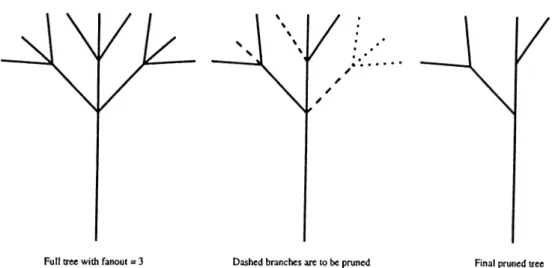
Full tree with fanout = 3 Dashed branches are to be pruned

Dotted branches are implicitly pruned because of their parents

Final pruned tree

Figure 3.3. Stochastic Pruning of Branches

Statistical self-similarity provides non-identical sub-trees bearing resem­ blance to other sub-trees and the whole tree. This feature adds a natural visual aspect to the model. Furthermore, stochastic pruning of branches is in­ troduced into the model. Paraphrased, initial branch count is used to distribute the sibling branches equally inside the branch cone, but some of the proposed branches are pruned randomly to enhance the natural aspects and suppress the regularity of the model. Figure 3.3 provides a 2D example of pruning. The dashed branches in the middle tree are to be pruned. The selection is based on a random survival-of-the-fittest. With certain probabilities, some branches are pruned down. The dotted branches are siblings of the pruned ones, which are therefore implicitly pruned.

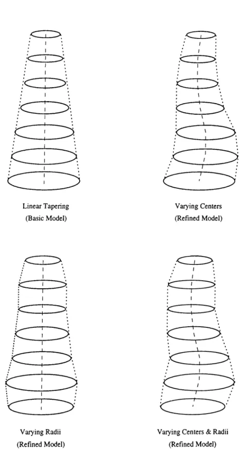
Further refinements are made to the fleshing-out of the branches. Initially, in the basic model (Section 3.1), branches are assumed to be simple gener­ alized cylinders with tapering. Further enhancements are introduced in the refined model. Each branch starts off as in the basic model, but it is perturbed stochastically to provide a more natural appearance. The discs are sampled or­ thogonally at constant, uniform intervals along the straight branch axis. Then the centers of these discs are transformed in 3D using a mean and variance of displacement along the orthogonal axes. Thus, the straight cylinder axis becomes distorted with random perturbations to its linearity. A second en­ hancement is varying the linearly tapered disc radii. The mean radius length

CHAPTERS. THE MODEL ₁₇

is computed by linearly interpolating between the bottom and top radii as in the basic model. A variance is introduced into the radii length to deform the smooth linear tapering of cylindrical branches. This feature provides a wig- gly appearance, accounting for the non-linear local enlarging of branch trunks. (See Figure 3.4 for details).

3.3

T h e T im e-A w a re M od el

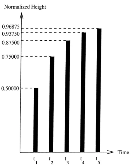
So far, both of the proposed models are good for still tree structures with a preset depth and level-wise branch count. Our scope, however, covers the growth animation of trees as well. Hence, we propose time-awareness of the re­ fined model to provide key-frames for discrete time values. Time is interpreted as a parameter in evaluating the final depth of recursion. Furthermore, both global time and local depth of a branch are used in computing the scale ratio of branches with respect to other levels. A heuristic involved in the process is that a branch grows to its theoretical (initially preset) maximum size log­ arithmically. This provides fast initial growth, dampening as the branch gets older. This scale factor is used for the height and the radius of the branches. Application to both dimensions keeps the branches at nearly constant aspect ratio at different time values. Another heuristic employed in the model is that the cone, in which the sibling branches are distributed, enlarges in time to mimic the weight of the growing child branches.

The time-awareness enhancement to the refined model provides an easy means of generating key-frames for growth animation. Recursion depth is proportional to the time value. The scale factor is a function of both. If a level is added every n units of time, the scale factor reaches 0.5 in n/2 time units, dampening logarithmically. In other words, it becomes 0.75 at n time units, and proceeds to 0.875 at 2n time units. After 4n time units, when the next level of branches are born, the previous layer reaches 93.75% of its full size. This heuristic logarithmic growth pattern is implemented for n = 4 with pleasing results. (See Figure 3.5).

Implementation details of the time-aware model and the real-time graphical user interface are presented in Chapter 4.

CHAPTERS. THE MODEL ₁₈

. C

c :

c >·. .< Z J Z > . C

c

C _ r 3 > , r > · Linear Tapering (Basic Model) Varying Centers (Refined Model)

C

:<Z

c

c

Varying Radii (Refined Model)

Varying Centers & Radii (Refined Model)

CHAPTERS. THE MODEL 19 Normalized Height

A

0.96875 0.93750 0.87500 0.75000 0.50000 ---Time t t t t t 1 2 3 4 5

C h a p te r 4

Implementation

We propose a time-aware model for fractal tree structures in Chapter 3. The main concern of the model is fast construction and rendering. The model is implemented on Silicon Graphics Iris Indigo XS24 workstation^. Real-time user interaction is regarded as the main concern throughout the implementation phase.

We present implementation details about the model itself in Section 4.1. Section 4.2 presents the features of the real-time graphical user interface im­ plemented under X-Windows using the Motif 1.2 widget set.

4.1

Im p lem en ta tio n o f th e T im e-A w are M o d el

The Time-Aware Model is an enhanced version of the Refined Model presented in Figure 3.2. The recursive core is kept with modifications to account for the time dependency. The Refined Model facilitates individual random number generators for all stochastic parameters so that bcisic form of the entire tree stays consistent over varying time values.

^ Entry level SGI workstation in 1992.

CHAPTER 4. IMPLEMENTATION ₂₁

4.1.1

C o n stru ctio n

Branch construction starts at the origin of the 3D space. The initial branch axis is in the positive 2:-axis direction. Discs are sampled at equal intervals along its length orthogonally. Next phase varies the linearly varied radii of the discs to provide the wiggly appearance. Finally, center points are translated in the xy-plane so that discs are shifted out of uniform order. Translating the center points in the positive .s-axis direction enlarges the patches on the surface of the generalized cylinder branches. This is an unwanted effect which distorts the rendered view. Therefore, translation of the centers is confined to the xy-plane.

After the distortion of the layout of the discs, points are sampled on their perimeters yielding regular polygons orthogonal to the positive z-axis. These polygons are stacked on top of each other constituting discrete control points for the surface of the branch.

The branch is modeled as a collection of discrete surface control points. These points are then moved to their appropriate position in space relative to the overall tree structure using linear transformations [11] [31].

This procedure for generating control points for branches simplifies the construction of the tree. This is desirable as the core concern is speed in the generation process. The transformation matrix is computed only once for each disc along a branch. Scaling is performed on the original branch at the origin. This renders the single transformation matrix possible because relative placement is already accounted for. The transformation then becomes simple rotations and translations to locate the branch at its appropriate place and correct orientation with respect to the parent branch.

Branches are generated in a depth-first manner due to the implicit ordering of recursion. However, this presents no inconvenience for the construction process. The data structure (presented shortly) renders it possible to preserve adjacency relationships between parent and sibling branches.

CHAPTER 4. IMPLEMENTATION ₂₂

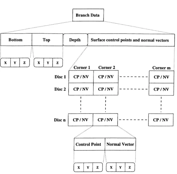
Figure 4.1. Data Structure for a Branch

The D ata Structure

As presented in Section 4.1.1, the tree consists of branches which are in turn represented by control points sampled on their surfaces. We also need the recursion depth level, and the branch axis bottom and top points as described in Section 4.2. Rendering phase needs, not only the control points, but also the normal vectors at these points for correct shading. Therefore, data required for a branch is a contiguous array of (control point, normal vector) pairs defining the surface (See Figure 4.1). The data structure for the tree model is implicitly a tree version. The important feature is that each node has variable fan-out. Therefore, we need a generalized tree data structure.

CHAPTER 4. IMPLEMENTATION ₂₃

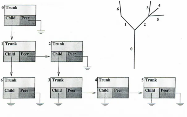
As discussed in Section 4.1.2 and presented in Figure 4.1, branches are stored as individual entities. They do not e.xhibit any kind of relationship with their parent, peer and offspring branches. The adjacency has to be accounted for so that the final visualization can identify the entire tree as a single object. The unifying data structure is presented in Figure 4.2, where each branch of the tree on the right is represented by a box on the left. Each box contains three pointers; namely one for the branch data (Trunk), one for the first child branch, and one for the peer branch. The rendering phase traverses the tree breadth-first, visiting peer branches before progressing to the siblings.

Figure 4.2. Generalized Tree Data Structure

Without disregarding the speed concern, we need a fast solution for the intersection of generalized cylinders problem. The problem arises at branch intersection points. Even for just two branches meeting at a junction, since they are neither collinear nor parallel, they cannot maintain the continuity expected of natural branch connections. Therefore, a heuristic solution has been adopted (See Figure 4.3). The primary axis top of a parent branch is adjacent to the axis bottom of the offspring branch. As we have sampled points on discs along the branches, we use them to create a pseudo-interconnection. The discs involved are the second top-most in the parent and the second bottom-most in the sibling. During the rendering process, a wedge is formed traversing the

CHAPTER 4. IMPLEMENTATION ₂₄

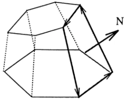
points on the two discs in counter-clockwise fashion (See Figure 4.4). This ensures that no hole is left at the interconnection node. Rendering details are given in Section 4.1.2.

Axis of child branch

Figure 4.3. Wedge Formation at Branch Intersections

This heuristic solution to branch intersections enforces a refinement in the data structure. Each branch must have a link to all of its siblings. Since the number of siblings are not exactly known beforehand^, the data structure needs to be flexible.

We propose a tree structure with nodes having three pointers. One pointer is for the contiguously allocated branch surface control points. The other two pointers are for the first child and the first peer branch. Therefore, to reach all first level siblings, a branch follows its first child link followed by the peer link of that child until no more child peers are available. This data structure

CHAPTER 4. IMPLEMENTATION 25

Figure 4.4. Wedge surface consists of patches generated by visiting the corners counter-clockwise

is easy to construct and provides all of the flexibility we need for the rendering phase.

M e th o d E xp lan atio n

Line Approximated axis drawn between bottom and top centers D isc Polygons sampled as cross-sections of the branch

W ire fra m e Control points on the branch surface connected

S h ad ed Polygons in the wireframe structure Gouraud [10] shaded T e x tu re d Polygons in the wireframe structure texture mapped

Table 4.1. Rendering Methods

4 .1 .2

R endering

The model is implemented on a Silicon Graphics Iris Indigo XS24 workstation with the IrisGL library [1] [16] [17] used in the rendering process. User interface is implemented under X-Windows [18] [19] with the Motif widget set [20] [21].

Various levels of rendering are implemented for easy manipulation of large trees as well as small ones. The rendering methods are given in Table 4.1. These different rendering techniques are also utilized in user interaction as described in Section 4.2.

The rendering process is five-fold. For the line case, we only need the bottom and top center points for each branch. Connecting these points by

CHAPTER 4. IMPLEMENTATION ₂₆

straight line segments, we get a skeletal tree which provides an idea about the final form. As it is the fastest to generate — consisting of line segments only — the line method is ideal for preview purposes encountered in user interaction.

The disc model provides a cross-sectional view which is useful when manip­ ulating trunk parameters like branch width and related ratios. It actually uses all of the data generated in the construction phase. The discs are rendered as polygons consisting of the sampled points. The disc method is also a fast rendering scheme, because it only consists of line segments as in the previous case.

The wireframe method connects the discs of the previous case, forming the branch surfaces. It also shows the wedges formed to cover the branch intersections. With this feature added, it is good for previewing the actual form of the final tree.

The shaded model is based on the wireframe model. The IrisGL library provides hardware accelerated Gouraud[10] shading with at most eight light sources. The normal vectors computed at the construction phase are utilized to speed up the rendering.

The final rendering method is texture mapped. This is based on the shad­ ing method with the addition of a simple bark texture to enhance the visual impact. IrisGL provides library calls to simplify texture mapping. Texture map corner coordinates are related with surface patch corners. Pre-computed normal vectors enhance the texture mapping with shading. This method takes more time than all others but provides the best visual results.

4.2

R ea l-T im e G raphical U ser Interface

Within the scope of the thesis, we implement a system to design, render and animate fractal tree models conforming with the Time-Aware Model. The main concern is near real-time response with maximum interactivity.

CHAPTER 4. IMPLEMENTATION ₂₇

Button Axis Direction Action

Left Horizontal Vertical Left Right Up Down

Rotation around 2:-axis Rotation around i-axis Rotation around x-axis Rotation around i-axis

Middle Horizontal Left N/A

Right N/A

Vertical Up Zoom in

Down Zoom out

Right Horizontal Left Rotation around y-axis Right Rotation around y-axis

Vertical Up Rotation around i-axis

Down Rotation around x-axis

Table 4.2. Mouse Actions

widget set. Mixed mode programming^ enables standard Motif drawing win­ dows to be accessed through GL. Hence, Motif provides the framework to build on.

GUU construction extends beyond widget creation and placement. Our system approaches the interaction problem with the mouse in mind as proposed by Ozgiig [23]. Keyboard interaction is usually slow and difficult to learn or remember. On the other hand, the mouse is simple and fast to use. On­ screen sliders are chosen to easily manipulate various numerical parameters. These sliders provide near real-time preview. All parameters except for those related to the branch radius are previewed in the line rendered mode. For the rest, the preview mode is the disc method, because of the cross-sectional view. Moreover, the construction phase also optimizes itself to produce data for the related preview mode. The line rendering mode needs only the branch axis bottom and top points. The constructor makes use of this fact to skip the generation of surface control points, which speeds up the building phase considerably.

The power of the interaction mechanism, however, lies with the interaction possible within the visualization window. The tree image is rendered in a GL

^IRIS documentation refers to hybrid programs that use GL and X-Windows as mixed mode programs.

CHAPTER 4. IMPLEMENTATION 28

sub-window where the mouse has special functions.

Usually, 3D controls are difficult to manage with a 2D pointing device like the mouse. We use the 3-button mouse installed on SGI workstations to rotate and scale the tree. The mouse buttons are used in conjunction with dragging to give the feeling of holding and transforming the tree model in the object space. The mapping between the mouse events and the linear transformations is given in Table 4.2.

When the rendering method is shaded or texture mapped, the rendering time usually takes too long to allow fast interaction. As described in Section 4.1.2, line method is the fastest to complete. Therefore, the rendering mode switches to line when user interaction is detected in the form of a mouse drag. Thus, the system manages to respond in near real-time to rotations and scal­ ings. Once the drag stops, the original mode is restored to provide the desired image.

Render mode switching in structure preview and user interaction makes near real-time system response possible. This is an important issue for an ergonomic interface. Avoiding the keyboard and concentrating on the mouse, the user easily focuses on the tree model parameters and the image rendered in the viewing window.

C h a p te r 5

Conclusion

Tree modeling poses many challenges when subjected to fast construction. Heuristic methods are vital for a tree modeling system which must provide near real-time user interaction both in construction and rendering phases.

We have presented such a system capable of generating time dependent tree models with statistical self-similarity, stochastic branch pruning, and deformed branch structures.

The Time-Aware Model is the result of many heuristic short-cuts. We model the branches as generalized cylinders. We assume the cylinders have polygonal lateral surfaces which are further sampled at regular intervals along the main cylinder axis. This provides a mesh model of the generalized cylinder, or branch. At this abstraction level, we can deform the regular polygonal cylinders randomly to get more realistic images. The perturbations on the centers and radii of branches provide the desired realism with natural wiggly appearance.

Improvements on the deformation of branches are possible through bending and twisting. In our model, the branch axis is assumed to be linear at first. As a result of the random variations in disc centers, the linear axis becomes zig-zag. Initially bending the axis can provide branches that point down in contrast to up-going branches currently available. Twisting along the axis can also generate flowing trunk patterns which might be desirable. Incorporating pysical laws to compensate for external forces like gravity and wind conditions

CHAPTERS. CONCLUSION ₃₀

can be fruitful. Bending in the reverse direction of gravity or in conformation with directed wind effect can enhance the realism. Stiffness coefficient can be used as a factor to improve the natural flavor of bending. Old branches, assumed to be stiffer than younger off-shoots, can be made more resistive to external forces, thus conforming with nature. These improvements add only minor compexity to our near real-time model.

A major problem is faced at branch intersection points. The actual problem is intersection of generalized cylinders. With our polygonal mesh defined on the lateral surface of the cylinders, it is possible to speed up intersection gen­ eration heuristically. Instead of creating the intersection set of the branches, we prefer post-processing of the model through means of creating parametric wedges to fill in the gaps which occur at intersection of branches pointing in different directions. Our data structure provides for quick implementation of the problem because each parent branch can access the discs of any number of its siblings. Thus, after rendering the branches which take part in the in­ tersection, wedges are constructed and rendered over the intersection point. Using backface culling and z-buffer, it is possible to omit unwanted parts of the wedges from the final image.

Time dependence of the tree model for growth animation is managed through the use of simulated time as a parameter for branch length and recursion level computations. A heuristic is employed for branch length calculations. Logarithmic growth is assumed for aging branches. Furthermore, the cone in which the sibling branches are distributed enlarges with increasing time. These heuristics provide a fast modeling of aging of trees. Since the time-aware model lacks botanic facts, enhancements are possible through introduction of rules from botany.

Future work can be conducted in providing additional features to enhance the realism possible with the current system. Key frames that can be gener­ ated at discrete time values can be interpolated both internally and through the use of third-party animation packages. Current rendering is based on the IrisGL library which provides Gouraud shading with simple texture mapping. More realistic images are possible if the model is rendered using ray-tracing or radiosity packages. However, such packages render the near real-time user interaction impossible due to the amount of computations involved.

A p p e n d ix A

Color Plates

In the following pages, color plates are presented which exemplify the rendering modes and the aging simulation. First five plates show the line, disc, wireframe, shaded and texture mapped tree models. The following five plates are of an example aging sequence of a tree.

APPENDIX A. COLOR PLATES ₃₂ '.ill I 2 ·> 0 I I u n k 1 c n < | t h . t h H .«t i « 2 0 H o t t o w l< -«<1 i u s 1 (> I o| > R .kI i II s . 80 W i <11 li R a t i o 6 0 S t. <> w - n I a I K ' li A i K | I <> tt H o t II t s 2 il R I a IK' li o s 2 8 I i w · · < >

siiAi)i:i) riixiuRi; uui r

/.

APPENDIX A. COLOR PLATES 33 /rr*r 2b 0 I I IIII k 1 i ‘ M<| t li . /b I . «' iK| I li H * * » > <> 3 0 H o i t o m K,i<l i u s 1 (> l o p H a i i i u s . 8 0 H i <11 h K a I i o 6 0 St o » - n I a i j c l i An»| I o 8 N D i s c s 8 I P o i n t s 3 N H i . ) II c li o s 2 S IKXIURK QUIT Z

AÖ

A

, % % t / ’> 10 0 . ( 1 0 0 . (

APPENDIX A. COLOR PLATES 34 y [ I l i n k I o n «It h . /b I.«-n<i t h K .11 i o 2 0 H o l t o w K .«<1 i II s 1 (> lop R .kI ins . 8 0 H i <11 h R n t i O 6 0 S t o w - Hi . i n o i l An<i 1 « 4 P o i I I ! s 2 4 Ri . i n c h < > s 2 8 I I MO < S H A D K I ) r i l X H J R K Q U \ T 7.

APPENDIX A. COLOR PLATES ₃₅ I f r v t : -JJ 2\> 0 l i u n k l o n q t . h . 7 b l . o i Kf t h R a t i o 20 Hot . t o m R a d i u s 1 () Г о |> R a <1 i u s .80 W i d t h R a t i o 60 S t o n i - B i . « n c h An<il€> 8 M Discs 8 (t V o i II t. s 2 N 1И a I I о l i e s ->8 lime < > {.INK I ' HXTURK Q U I T

J

APPENDIX A. COLOR PLATES ₃₆ fn r 0 I I l i n k I <>n<| t h . /·* f,<'iM| t li H .11 I o /0 H o t t o » H . lA I II K 1 f> l o | > K . i i l i i i s . 80 W i d t h R. i t i o (>0 S t l i m - i i i . i n c h A n < | I c M I' o i n t s I H I .1 n r h c s I 1 n .■ S HAD hi) I h X n J H h QU I I %

!?>■

'i . ! > H I \ h i f ' % / 'i: %

nr

10 0 . ( 1 00 . (

APPENDIX A. COLOR PLATES ₃₇ uj zi.o I I l i n k 1 oi K| t . Ii . Vb I, n <j t h H .· t. i o ?.() h o t . t o » R a i l i n s 1 () i o | > R .kI i n s . 80 W i <11 h R a t i o 60 St. o i B - B i a n c h A m | 1 « 8 N D i s c s 8 ii P o i n t. s 2 tt B l a n c h c s 10

SHADKD IMXTURi; QUIT

Z

APPENDIX A. COLOR PLATES ₃₈ ; — » f r e t ' A1 2!>() I 1 l i n k . /b If« I) t h R a t. i o ' H o I. t o m R a <1 i u s 1 (> ' l' o| > R a<i i u s . 8 0 Wi<U. li R a t i o 60 IS t . o m - H i a i i c l i An<i 1 « ^ a tt D i s c s 8 N P o i n t s 2 H R i a n c h o s 2 0 l i m e < > T E X T U R K Ü U I T Z

APPENDIX A. COLOR PLATES 39 lij 0 I i l i n k 1 « n < i t h ./U I· o II <11 h K a t. i o 2 0 1^01.1.om Radius 1 (> To|> Radius . . 8 0 W i <11. Ii R a t. i o 60 St. « w - B i a n c l i A t i < | l « 8 M D i s c s 8 II Do i n t. s ?. H Hi a n d i e s ?.'1 Time

S H ADKD TKXTURh: QOIli Z T 'I 1/ " - 4 V

■'y

/

4 /·

APPENDIX A. COLOR PLATES ₄₀ U 2 b 0 I T I l i n k h i i . / b • L < ^ n < | t l > K a t . i o I ^ 2 0 I B o t t o m R a < l i U K I I 1 < > | > K a < i i u K . 8 0 H i t . I i R a t . i o 60 | S t . « m - B i a n c h A n q 1 « 8 i ■ ■ t t I ) i K c K 8 # P o i n t , s j 2 I I B i a n c h o N 28 I 1 i m« < > I ) I S C T K X T U R K O U I T z \ l · ' K

t

4

r

'·■- i V

i ‘■‘r

rr

■y . . . c . , 10 0 . ( 10 0 . (

J

APPENDIX A. COLOR PLATES ₄₁ I /П 'С 2b 0 I I l i n k 1 o n q t h . /Ь I. oi Ki t h R a t i о 20 Dot . t om R <i<I i n s 1 () I о |> R a d i n s .80 W i <! t. h R a t i o 60 i St. o m - R i a n c h An<) 1 о 8 i) Discs 8 N P o i n t , s 2 M IH . m e l i e s i2 l i m e -UJ

A p p e n d ix B

Fractal Similarity Concepts

When we refer to similarity in fractals, various concepts arise including self­

similarity and self-affinity with their exact and statistical forms. We present

a formal definition of the said terms [5].

The similarity transformation transforms points x = (x i,...^x e) in E-

dimensional space into new points x' = (rxi, ...,rxE) with the same value of the scaling ratio r. A bounded self-similar fractal set of points S is self-similar with respect to a scaling ratio r if is the union of N non-overlapping subsets

Si,...,Sn, ^dch of which is congruent to the set r[S) ontained from S by the

similarity transform defined by 0 < r < 1. Here congruent means that the set of points Si is identical to the set of points r[S) after possible translations and/or rotations of the set. The similarity dimension is then given by

Ds = \n N

In i_T

(

1

)

The set S is statistically self-similar when S is the union of N distinct subsets each of which is scaled down by r from the original and is identical in all statistical respects to r(S). Often, random sets — such as a coastline — are statistically self-similar not only for a given value of the scaling ratio r, but for all scaling ratios above some lower cutoff (the micro-scale) and some upper cutoff (the macro-scale).

An affine transformation transforms a point x = ( x i,..., x e) into new points

APPENDIX B. FRACTAL SIMILARITY CONCEPTS 43

x' — {riXi, ...^veXe), where the scaling ratios ri,...,rE are not all equal.

A bounded set S is self-affine with respect to a ratio vector r = (rj, ...,rE) if S is the union of N non-overlapping subsets Si,...,Sn, each of which is

congruent to the set r(5') obtained from S by the affine transform defined by r. Here congruent means that the set of points Si is identical to the set of points r(5') after possible translations and/or rotations of the set.

The set S is statistically self-affine when S is the union of N non-overlapping subsets each of which is scaled down by r from the original and is identical in all statistical respects to r(5). The fractal dimension of even the simplest self-affine fractals is not uniquely defined.

BIBLIOGRAPHY ₄₅

[12] J. D. Foley, A. van Dam, S. K. Feiner, and J. F. Hughes. Computer

Graphics. The Systems Programming Series. Addison-Wesley, 2nd edition,

1990.

[13] Y. Kawaguchi. A morphological study of the nature. Computer Graphics.! 16(3):223-232, 1982.

[14] A. Lindenmayer. Mathematical models for cellular interaction in devel­ opment. Journal of Theoretical Biology, 8:280-315, 1968. Parts I and II.

[15] B. B. Mandelbrot. The Fractal Geometry of Nature. W. H. Freeman, San Francisco, 1982.

[16] P. McLendon. Graphics Library Programming Tools and Techniques. Sil­ icon Graphics Inc., Mountain View, CA, 1991. Document Number 070- 1489-010.

[17] P. McLendon. Graphics Library Programming Guide. Silicon Graphics Inc., Mountain View, CA, 1992. Document Number 007-1210-050.

[18] A. Nye and T. O’Reilly. X Toolkit Intrinsics Programming Manual, vol­ ume 4. O ’Reilly L· Associates, Inc., osf/motif 1.2 edition, 1992.

[19] A. Nye and T. O’Reilly. X Toolkit Intrinsics Reference Manual, volume 5. O ’Reilly & Associates, Inc., osf/motif 1.2 edition, 1992.

[20] Open Software Foundation, Cambridge, MA. OSF/M otif Programmer’s

Guide, release 1.1 edition, 1991.

[21] Open Software Foundation, Cambridge, MA. OSF/M otif Programmer’s

Reference, release 1.1 edition, 1991.

[22] P. E. Oppenheimer. Real time design and animation of fractal plants and trees. ACM SIGGRAPH, 20{4):55-64, 1986.

[23] B. Özgüç. Thoughts on user interface design for multi window envi­ ronments. In E. Gelenbe and A. R. Kaylan, editors, Second Interna­

tional Symosium on Computer and Information Sciences, pages 477-488,

BIBLIOGRAPHY 46

[24] P. de RefFye, C. Edelin, J. Frangon, M. Jaeger, and C. Puech. Plant models faithful to botanical structure and development. ACM Computer

Graphics^ 22(4):151-158, August 1988.

[25] P. Prusinkiewicz, A. Lindenmayer, and J. Hanan. Developmental models of herbaceous plants. ACM Computer Graphics, 22(4):141-150, August

1988.

[26] P. Prusinkiewicz. Applications of 1-systems to computing imagery. In

Proceedings of the Third Workshop on Graph Grammars and their Appli­ cations to Computer Science, pages 534-548, Warranton, December 1986.

[27] P. Prusinkiewicz and J. Hanan. Lindenmayer Systems, Fractals, and Plants, volume 79 of Lecture Notes in Biomathematics. Springer-Verlag,

1989.

[28] P. Prusinkiewicz and A. Lindenmayer. The Algorithmic Beauty of Plants. Springer-Verlag, 1990.

[29] W. T. Reeves and R. Blau. Approximate and probabilistic algorithms for shading and rendering structured particle systems. Computer Graphics,

19(3):313-322, 1985.

[30] A. R. Smith. Plants, fractals and formal languages. Computer Graphics, 18(3):1-10, 1984.

[31] A. Watt. Fundamentals of Three-Dimensional Computer Graphics.