A new method in object lighting : using surface chromaticity coordinates as a led-based lighting tool in museums

(1)

Pair 38 S_7_1 - S_7_3 _.559 _1.481 _.254 _.042 _1.076 _2.200 ₃₃ _.035 Pair 39 S_7_1 - S_7_4 1.559 1.691 .290 .969 2.149 5.375 33 .000 Pair 40 S_7_2 - S_7_3 -1.206 1.473 .253 -1.720 -.692 -4.775 33 .000 Pair 41 S_7_2 - S_7_4 -.206 1.572 .270 -.754 .343 -.764 33 .451 Pair 42 S_7_3 - S_7_4 _1.000 _1.073 _.184 _.626 _1.374 _5.434 ₃₃ _.000 Pair 43 S_8_1 - S_8_2 _2.206 _1.038 _.178 _1.844 _2.568 _12.391 ₃₃ _.000 Pair 44 S_8_1 - S_8_3 .912 1.422 .244 .416 1.408 3.739 33 .001 Pair 45 S_8_1 - S_8_4 1.118 1.493 .256 .597 1.638 4.366 33 .000 Pair 46 S_8_2 - S_8_3 _-1.294 _1.244 _{.213 -1.728} _-.860 _-6.066 ₃₃ _.000 Pair 47 S_8_2 - S_8_4 -1.088 1.379 .236 -1.569 -.607 -4.602 33 .000 Pair 48 S_8_3 - S_8_4 .206 1.298 .223 -.247 .659 .925 33 .362

(2)

APPENDIX G.3: Paired T-Tests for Saturation.

Table G.3. Paired Samples Test for Saturation.

Paired Differences t df Sig. (2-tailed) Mean Std. Deviat ion Std. Error Mean 95% Confidence Interval of the Difference Lower Upper Pair 1 S_1_1 - S_1_2 1.794 1.274 .218 1.350 2.239 8.212 33 .000 Pair 2 S_1_1 - S_1_3 .324 1.492 .256 -.197 .844 1.265 33 .215 Pair 3 S_1_1 - S_1_4 .588 1.844 .316 -.055 1.232 1.860 33 .072 Pair 4 S_1_2 - S_1_3 _-1.471 _1.237 _{.212 -1.902 -1.039} _-6.934 ₃₃ _.000 Pair 5 S_1_2 - S_1_4 -1.206 1.250 .214 -1.642 -.770 -5.625 33 .000 Pair 6 S_1_3 - S_1_4 .265 1.639 .281 -.307 .836 .942 33 .353 Pair 7 S_2_1 - S_2_2 1.794 .880 .151 1.487 2.101 11.887 33 .000 Pair 8 S_2_1 - S_2_3 _.559 _1.481 _.254 _.042 _1.076 _2.200 ₃₃ _.035 Pair 9 S_2_1 - S_2_4 .941 1.808 .310 .310 1.572 3.035 33 .005 Pair 10 S_2_2 - S_2_3 -1.235 1.281 .220 -1.682 -.788 -5.625 33 .000 Pair 11 S_2_2 - S_2_4 -.853 1.654 .284 -1.430 -.276 -3.007 33 .005 Pair 12 S_2_3 - S_2_4 _.382 _1.724 _.296 _-.219 _.984 _1.294 ₃₃ _.205 Pair 13 S_3_1 - S_3_2 _1.853 _1.132 _.194 _1.458 _2.248 _9.547 ₃₃ _.000 Pair 14 S_3_1 - S_3_3 1.059 1.434 .246 .558 1.559 4.305 33 .000 Pair 15 S_3_1 - S_3_4 .824 1.660 .285 .244 1.403 2.893 33 .007 Pair 16 S_3_2 - S_3_3 _-.794 _1.366 _{.234 -1.271} _-.318 _-3.390 ₃₃ _.002 Pair 17 S_3_2 - S_3_4 -1.029 1.586 .272 -1.583 -.476 -3.786 33 .001 Pair 18 S_3_3 - S_3_4 -.235 1.634 .280 -.805 .335 -.840 33 .407 Pair 19 S_4_1 - S_4_2 .647 1.346 .231 .178 1.117 2.804 33 .008 Pair 20 S_4_1 - S_4_3 _-.588 _1.635 _{.280 -1.159} _-.018 _-2.098 ₃₃ _.044 Pair 21 S_4_1 - S_4_4 -.824 1.898 .326 -1.486 -.161 -2.529 33 .016 Pair 22 S_4_2 - S_4_3 -1.235 1.415 .243 -1.729 -.741 -5.089 33 .000 Pair 23 S_4_2 - S_4_4 -1.471 1.461 .251 -1.980 -.961 -5.868 33 .000 Pair 24 S_4_3 - S_4_4 -.235 1.776 .305 -.855 .384 -.772 33 .445 Pair 25 S_5_1 - S_5_2 _2.324 _.768 _.132 _2.056 _2.591 _17.652 ₃₃ _.000 Pair 26 S_5_1 - S_5_3 .765 1.156 .198 .361 1.168 3.856 33 .001 Pair 27 S_5_1 - S_5_4 1.647 1.252 .215 1.210 2.084 7.668 33 .000 Pair 28 S_5_2 - S_5_3 _-1.559 _.991 _{.170 -1.904 -1.213} _-9.176 ₃₃ _.000 Pair 29 S_5_2 - S_5_4 _-.676 _1.224 _{.210 -1.104} _-.249 _-3.223 ₃₃ _.003 Pair 30 S_5_3 - S_5_4 .882 1.274 .218 .438 1.327 4.040 33 .000 Pair 31 S_6_1 - S_6_2 1.353 1.203 .206 .933 1.773 6.557 33 .000 Pair 32 S_6_1 - S_6_3 _-.176 _1.783 _.306 _-.799 _.446 _-.577 ₃₃ _.568 Pair 33 S_6_1 - S_6_4 _-.471 _1.674 _{.287 -1.055} _.113 _-1.639 ₃₃ _.111 Pair 34 S_6_2 - S_6_3 -1.529 1.354 .232 -2.002 -1.057 -6.588 33 .000 Pair 35 S_6_2 - S_6_4 -1.824 1.114 .191 -2.212 -1.435 -9.546 33 .000 Pair 36 S_6_3 - S_6_4 -.294 1.426 .244 -.792 .203 -1.203 33 .238 Pair 37 S_7_1 - S_7_2 _1.765 _1.075 _.184 _1.390 _2.140 _9.574 ₃₃ _.000

(3)

Pair 38 B_7_1 - B_7_3 _.529 _1.285 _.220 _.081 _.978 _2.403 ₃₃ _.022 Pair 39 B_7_1 - B_7_4 1.471 1.502 .258 .946 1.995 5.708 33 .000 Pair 40 B_7_2 - B_7_3 -1.588 1.184 .203 -2.001 -1.175 -7.824 33 .000 Pair 41 B_7_2 - B_7_4 -.647 1.495 .256 -1.169 -.125 -2.524 33 .017 Pair 42 B_7_3 - B_7_4 _.941 _1.127 _.193 _.548 _1.334 _4.871 ₃₃ _.000 Pair 43 B_8_1 - B_8_2 _2.235 _1.075 _.184 _1.860 _2.610 _12.127 ₃₃ _.000 Pair 44 B_8_1 - B_8_3 1.029 1.446 .248 .525 1.534 4.152 33 .000 Pair 45 B_8_1 - B_8_4 1.324 1.093 .187 .942 1.705 7.059 33 .000 Pair 46 B_8_2 - B_8_3 _-1.206 _1.225 _{.210 -1.633} _-.778 _-5.738 ₃₃ _.000 Pair 47 B_8_2 - B_8_4 -.912 1.357 .233 -1.385 -.438 -3.919 33 .000 Pair 48 B_8_3 - B_8_4 .294 1.528 .262 -.239 .827 1.122 33 .270

(4)

APPENDIX G.2: Paired T-Tests for Brightness.

Table G.2. Paired Samples Test for Brightness.

Paired Differences t df Sig. (2-tailed) Mean Std. Dev. Std. Error Mean 95% Confidence Interval of the Difference Lower Upper Pair 1 B_1_1 - B_1_2 _1.706 _1.219 _.209 _1.280 _2.131 _8.158 ₃₃ _.000 Pair 2 B_1_1 - B_1_3 .853 1.459 .250 .344 1.362 3.408 33 .002 Pair 3 B_1_1 - B_1_4 1.559 1.618 .277 .994 2.123 5.618 33 .000 Pair 4 B_1_2 - B_1_3 -.853 1.395 .239 -1.340 -.366 -3.564 33 .001 Pair 5 B_1_2 - B_1_4 _-.147 _1.690 _.290 _-.737 _.443 _-.507 ₃₃ _.615 Pair 6 B_1_3 - B_1_4 .706 1.426 .244 .208 1.203 2.887 33 .007 Pair 7 B_2_1 - B_2_2 1.765 1.046 .179 1.400 2.130 9.836 33 .000 Pair 8 B_2_1 - B_2_3 .794 1.452 .249 .288 1.301 3.189 33 .003 Pair 9 B_2_1 - B_2_4 1.206 1.719 .295 .606 1.806 4.089 33 .000 Pair 10 B_2_2 - B_2_3 _-.971 _1.425 _{.244 -1.468} _-.474 _-3.973 ₃₃ _.000 Pair 11 B_2_2 - B_2_4 -.559 1.709 .293 -1.155 .037 -1.907 33 .065 Pair 12 B_2_3 - B_2_4 .412 1.635 .280 -.159 .982 1.468 33 .151 Pair 13 B_3_1 - B_3_2 _1.765 _1.046 _.179 _1.400 _2.130 _9.836 ₃₃ _.000 Pair 14 B_3_1 - B_3_3 _.794 _1.737 _.298 _.188 _1.400 _2.666 ₃₃ _.012 Pair 15 B_3_1 - B_3_4 .618 1.843 .316 -.025 1.261 1.955 33 .059 Pair 16 B_3_2 - B_3_3 -.971 1.359 .233 -1.445 -.496 -4.164 33 .000 Pair 17 B_3_2 - B_3_4 _-1.147 _1.438 _{.247 -1.649} _-.645 _-4.650 ₃₃ _.000 Pair 18 B_3_3 - B_3_4 _-.176 _1.604 _.275 _-.736 _.383 _-.641 ₃₃ _.526 Pair 19 B_4_1 - B_4_2 .529 1.354 .232 .057 1.002 2.280 33 .029 Pair 20 B_4_1 - B_4_3 -.441 1.795 .308 -1.068 .185 -1.433 33 .161 Pair 21 B_4_1 - B_4_4 -.765 1.908 .327 -1.430 -.099 -2.337 33 .026 Pair 22 B_4_2 - B_4_3 _-.971 _1.527 _{.262 -1.503} _-.438 _-3.706 ₃₃ _.001 Pair 23 B_4_2 - B_4_4 -1.294 1.605 .275 -1.854 -.734 -4.700 33 .000 Pair 24 B_4_3 - B_4_4 -.324 1.683 .289 -.911 .264 -1.121 33 .270 Pair 25 B_5_1 - B_5_2 2.147 .989 .170 1.802 2.492 12.661 33 .000 Pair 26 B_5_1 - B_5_3 _.765 _1.350 _.231 _.294 _1.236 _3.304 ₃₃ _.002 Pair 27 B_5_1 - B_5_4 1.559 1.440 .247 1.057 2.061 6.314 33 .000 Pair 28 B_5_2 - B_5_3 -1.382 1.074 .184 -1.757 -1.008 -7.509 33 .000 Pair 29 B_5_2 - B_5_4 _-.588 _1.438 _{.247 -1.090} _-.087 _-2.385 ₃₃ _.023 Pair 30 B_5_3 - B_5_4 _.794 _1.298 _.223 _.341 _1.247 _3.569 ₃₃ _.001 Pair 31 B_6_1 - B_6_2 1.294 1.219 .209 .869 1.720 6.189 33 .000 Pair 32 B_6_1 - B_6_3 .059 1.740 .298 -.548 .666 .197 33 .845 Pair 33 B_6_1 - B_6_4 -.529 1.813 .311 -1.162 .103 -1.703 33 .098 Pair 34 B_6_2 - B_6_3 _-1.235 _1.327 _{.228 -1.698} _-.772 _-5.428 ₃₃ _.000 Pair 35 B_6_2 - B_6_4 -1.824 1.336 .229 -2.290 -1.357 -7.956 33 .000 Pair 36 B_6_3 - B_6_4 -.588 1.373 .236 -1.067 -.109 -2.498 33 .018 Pair 37 B_7_1 - B_7_2 2.118 .844 .145 1.823 2.412 14.623 33 .000

(5)

Pair 23 H_4_2 - H_4_4 _-2.029 _1.425 _.244 _-2.526 _-1.532 _-8.307 ₃₃ _.000 Pair 24 H_4_3 - H_4_4 -.618 1.181 .203 -1.030 -.206 -3.049 33 .004 Pair 25 H_5_1 - H_5_2 2.471 .748 .128 2.210 2.732 19.256 33 .000 Pair 26 H_5_1 - H_5_3 1.147 .610 .105 .934 1.360 10.971 33 .000 Pair 27 H_5_1 - H_5_4 _2.147 _.925 _.159 _1.824 _2.470 _13.528 ₃₃ _.000 Pair 28 H_5_2 - H_5_3 _-1.324 _1.065 _.183 _-1.695 _-.952 _-7.245 ₃₃ _.000 Pair 29 H_5_2 - H_5_4 -.324 1.273 .218 -.768 .120 -1.482 33 .148 Pair 30 H_5_3 - H_5_4 1.000 .853 .146 .702 1.298 6.837 33 .000 Pair 31 H_6_1 - H_6_2 _1.706 _.906 _.155 _1.390 _2.022 _10.985 ₃₃ _.000 Pair 32 H_6_1 - H_6_3 .824 1.218 .209 .399 1.248 3.943 33 .000 Pair 33 H_6_1 - H_6_4 -.294 1.661 .285 -.874 .285 -1.032 33 .309 Pair 34 H_6_2 - H_6_3 -.882 1.149 .197 -1.283 -.482 -4.480 33 .000 Pair 35 H_6_2 - H_6_4 _-2.000 _1.557 _.267 _-2.543 _-1.457 _-7.490 ₃₃ _.000 Pair 36 H_6_3 - H_6_4 -1.118 1.343 .230 -1.586 -.649 -4.852 33 .000 Pair 37 H_7_1 - H_7_2 2.882 .409 .070 2.740 3.025 41.059 33 .000 Pair 38 H_7_1 - H_7_3 .941 .547 .094 .750 1.132 10.029 33 .000 Pair 39 H_7_1 - H_7_4 _1.941 _.600 _.103 _1.732 _2.151 _18.863 ₃₃ _.000 Pair 40 H_7_2 - H_7_3 _-1.941 _.343 _.059 _-2.061 _-1.821 _-33.000 ₃₃ _.000 Pair 41 H_7_2 - H_7_4 -.941 .547 .094 -1.132 -.750 -10.029 33 .000 Pair 42 H_7_3 - H_7_4 1.000 .426 .073 .851 1.149 13.675 33 .000 Pair 43 H_8_1 - H_8_2 _2.471 _.706 _.121 _2.224 _2.717 _20.391 ₃₃ _.000 Pair 44 H_8_1 - H_8_3 _1.471 _1.022 _.175 _1.114 _1.827 _8.390 ₃₃ _.000 Pair 45 H_8_1 - H_8_4 1.118 1.175 .201 .708 1.527 5.548 33 .000 Pair 46 H_8_2 - H_8_3 -1.000 1.181 .202 -1.412 -.588 -4.939 33 .000 Pair 47 H_8_2 - H_8_4 _-1.353 _1.276 _.219 _-1.798 _-.908 _-6.181 ₃₃ _.000 Pair 48 H_8_3 - H_8_4 -.353 1.346 .231 -.822 .117 -1.529 33 .136

(6)

APPENDIX G

DATA STRUCTURES17

APPENDIX G.1: Paired T-Tests for Hue.

Table G.1. Paired Samples Test for Hue.

Paired Differences t df Sig.

(2-tailed) Mean Std. Dev. Std. Error Mean 95% Confidence Interval of the Difference Lower Upper Pair 1 H_1_1 - H_1_2 _2.588 _.657 _.113 _2.359 _2.817 _22.978 ₃₃ _.000 Pair 2 H_1_1 - H_1_3 _1.118 _.591 _.101 _.911 _1.324 _11.025 ₃₃ _.000 Pair 3 H_1_1 - H_1_4 2.118 .686 .118 1.878 2.357 18.000 33 .000 Pair 4 H_1_2 - H_1_3 -1.471 .896 .154 -1.783 -1.158 -9.574 33 .000 Pair 5 H_1_2 - H_1_4 _-.471 _1.080 _.185 _-.847 _-.094 _-2.541 ₃₃ _.016 Pair 6 H_1_3 - H_1_4 1.000 .853 .146 .702 1.298 6.837 33 .000 Pair 7 H_2_1 - H_2_2 2.176 .716 .123 1.926 2.426 17.712 33 .000 Pair 8 H_2_1 - H_2_3 .824 1.114 .191 .435 1.212 4.311 33 .000 Pair 9 H_2_1 - H_2_4 1.676 1.319 .226 1.216 2.137 7.409 33 .000 Pair 10 H_2_2 - H_2_3 _-1.353 _1.041 _.179 _-1.716 _-.990 _-7.578 ₃₃ _.000 Pair 11 H_2_2 - H_2_4 -.500 1.503 .258 -1.024 .024 -1.940 33 .061 Pair 12 H_2_3 - H_2_4 .853 1.540 .264 .316 1.390 3.229 33 .003 Pair 13 H_3_1 - H_3_2 2.412 .783 .134 2.139 2.685 17.959 33 .000 Pair 14 H_3_1 - H_3_3 _1.147 _1.019 _.175 _.792 _1.503 _6.564 ₃₃ _.000 Pair 15 H_3_1 - H_3_4 .441 1.440 .247 -.061 .943 1.787 33 .083 Pair 16 H_3_2 - H_3_3 -1.265 .618 .106 -1.480 -1.049 -11.926 33 .000 Pair 17 H_3_2 - H_3_4 _-1.971 _1.141 _.196 _-2.369 _-1.572 _-10.069 ₃₃ _.000 Pair 18 H_3_3 - H_3_4 _-.706 _1.219 _.209 _-1.131 _-.280 _-3.376 ₃₃ _.002 Pair 19 H_4_1 - H_4_2 .794 1.067 .183 .422 1.166 4.340 33 .000 Pair 20 H_4_1 - H_4_3 -.618 1.577 .270 -1.168 -.068 -2.284 33 .029 Pair 21 H_4_1 - H_4_4 _-1.235 _1.689 _.290 _-1.825 _-.646 _-4.265 ₃₃ _.000 Pair 22 H_4_2 - H_4_3 _-1.412 _1.184 _.203 _-1.825 _-.999 _-6.955 ₃₃ _.000

17_{To manage the data, the conditions were coded. The letter stands for hue, saturation or brightness, the first digit} is the number of the color and the second digit is the number of box that the objects are located. For instance H_2_3 corresponds to the “result of preference of hue for the 2nd_{color (S3060-G50Y) in the 3}rd_{box” or “S_4_2} corresponds to the “result of preference of saturation for the 4th color (S3060-Y50R) in the 2nd_box.

(7)

APPENDIX F

(8)

D65 Reference 3000 K Created Light 4200 K 6500 K

S 3055 – R50B

S 3020 – B50G

S 3055 – B50G

(9)

APPENDIX E

THE LIT BOXES WITH COLORED OBJECTS

S 3060 – Y50R

S 3020 – Y50R

S 3060 – G50Y

(10)

APPENDIX D

TECHNICAL DRAWING OF DALI BOXES

Section A-A' Top View 30cm 3 0 c m Parallel

Side Elevation _{Front Elevation}

A A’ 2 6 ,4 c m 6cm 3 0 c m 7 c m 7 cm Magnet

(11)

APPENDIX C DEFINITION OF TERMS16

Chromaticity Coordinates: The ratio of each of the three stimulus values to their sum. The symbols recommended for the Chromaticity Coordinates are: x and y in the CIE 1931 standard colorimetric system. Color Temperature: Temperature of the full radiator that emits

radiation of the same chromaticity as the radiation considered. The unit is Kelvin. Correlated Color Temperature: The Color Temperature corresponding to the

point on the Planckian Locus, that is nearest to the point representing the chromaticity of the illuminant considered on an agreed uniform-chromaticity-scale diagram. The unit is Kelvin. Color Rendering Index: Measure of the degree to that the perceived

colors of objects illuminated by the source conforms to those of the same objects illuminated by a reference illuminant for specified conditions. The unit is Ra.

D65: D65 is a standard illuminant that represents

daylight with a Correlated Color Temperature of 6504 Kelvin.

(12)

APPENDIX B

(13)

NCS Natural Color System.

Nm Nanometers.

OIC Object Identification Card.

OIDA Optoelectronics Industry Development Association. Pc-LED Phosphor-coated Light Emitting Diode.

PN Junction Positive Negative Junction.

RGB LEDs Red Green Blue Light Emitting Diodes.

(14)

APPENDIX A

LIST OF ABBREVIATIONS

AlGaInP Aluminum Gallium Indium Phosphide.

CC Chromaticity Coordinates.

CCT Correlated Color Temperature.

CT Color Temperature.

CIBSE Chartered Institution of Building Services Engineers. CIE Commission Internationale de L’eclairage – International

Commission on Illumination.

CRI Color Rendering Index.

DALI Digital Addressable Lighting Interface.

DALI AG Digital Addressable Lighting Interface Activity Group. DIN Deutsches Institut für Normung (German Institute of

Standarts).

ICOM International Council of Museums.

IES Illuminating Engineering Society.

IESNA Illuminating Engineering Society of North America.

InGaN Indium Gallium Nitride.

IR Infrared Radiation.

LED Light Emitting Diode.

NCPTTC National Center for Preservation Technology and Training Committee.

(15)

Ventura, T. (n.d.). Psychoanalysis. Retrieved April 8, 2002, from http://allpsych.com/journal/psychoanalysis.html.

Wald, G, & Griffin, D. R. (1947). The change in refractive power of the human eye in dim and bright light. Journal of The Optical Society of America,

37(5), 321-336.

Williams, B. (2005). A history of light and lighting. Retrieved November 22, 2006, from http://www.mts.net/~william5/history/hol.htm.

Wyszecki, G., &. Stiles, W. S. (1982). Color science: Concepts and methods,

(16)

Osram: Incandescent Lamps. (n.d.). Retrieved February 28, 2005, from http://www.osram.com/service_corner/glossary/popups/17.html. Philips Lighting. (1993). Philips lighting manual (5th ed.). Eindhoven:

Lighting Design & Application Center.

Pridmore W. R., Huertas, R., Melgosa, M, & Negueruela, A, I. (2005). Discussion on perceived and measured wine color. Color Research &

Application, 30(2), 146-152.

Pridmore W. R. (2006). Effects of luminance, wavelength and purity on the color attributes: Brief review with new data and perspectives. Color

Research & Application, 32(3), 208-222.

Pridmore W. R. (2007). Effect of purity on hue (Abney Effect) in various conditions. Color Research & Application, 32(1), 25-39.

Quiet revolution may change the way we light our world. (2002). Retrieved February 1, 2007,from http://www.sandia.gov/media/NewsRel/ NR2002/LEDS2.htm.

Robilotto, R., & Zaidi Q. (2006). Lightness identification of patterned three- dimensional, real objects. Journal of Vision, 6, 18-36.

Scuello, M., Abramov, I., Gordon, J., & Weintraub, S. (2003). Museum lighting: Why are some illuminants preferred. Optical Society

of America Journal, 21(2), 306-11.

Scuello, M., Abramov, I., Gordon, J., & Weintraub, S. (2004). Museum lighting: Optimizing the illuminant. Color Research & Application,

29(2), 121-27.

Spagnoli, F. (2002). Color Kinetics Demonstrates Led-Based Intelligent White

Light Prototypes at Lightfair 2002. Retrieved January 31, 2007, from http://www.colorkinetics.com/corp/news/pr/archive/whitelight_proto.ht m?q=printme.

Steigerwald, D. A., Bhat, J. C., Collins, D., Fletcher, R. M. Holcomb, M. O., Ludowise, M. J., et al. (2002). Illumination with solid-state lighting technology. IEEE Journals on Selected Topics in Quantum

Electronics, 8(2), 310-320.

Stevens, J. C., & Stevens, S. S. (1963). Brightness function: Effects of adaptation. Journal of The Optical Society of America, 53(3), 375-385. The NCS System. (2002). Retrieved March 6, 2007 from http://83.168.206.

163/webbizz/mainPage/main.asp.

Thornton, W. A. (1992). Towards a more accurate and extensible colorimetry. Color Research & Application, 17, 79-122.

(17)

IES. (1984). IES lighting handbook: Reference Volume. New York: Illuminating Engineering Society of North America.

IES. (1987). IES lighting handbook: Application volume. New York: Illuminating Engineering Society of North America.

IES. (1996). IES museum and art gallery lighting: A recommended

practice. New York: Illuminating Engineering Society of North America. IESNA. (2000). IESNA lighting handbook: Reference and application. New

York: Illuminating Engineering Society of North America. Johnson, G. M., & Fairchild M. D. (2005). CRC: Chapter on visual

psychophysics and color appearance. Retrieved July 23, 2007, from page 3 at www.cis.rit.edu/fairchild/PDFs/PAP13.pdf.

Kaiser, P. K. (1996). Chromaticity diagram. Retrieved 15 January, 2006, from http://www.yorku.ca/eye/thejoy.htm.

Kerr, D. A. (n.d.). Color temperature. Retrieved November 11, 2006, from http://doug.kerr.home.att.net/pumpkin/Color_Temperature.pdf. Kesner, C. W. (1993). Museum exhibition lighting: Visitor needs and

perceptions of quality. Journal of Illuminating Engineering Society, 1, 45-55.

Kruithof, A. A. (1941). Luminescence Lamps for General Illumination. Philips

Technical Review, 6, 65-69.

Lighting Research Center. (1998). Museum lighting protocol project:

Archeology and collections series. New York: National Center for Preservation Technology and Training.

Melgosa, M., Rivas, M. J., Hita, E., & Vienot, F. (2000). Are we able to distinguish color attributes? Color Research & Application, 25(5), 356-367.

Muthu, S., Schuurmans, F. J. P., & Pashley, M.D. (2002). Red, Green and Blue LEDs for White Light Illumination. IEEE Journals on Selected

Topics in Quantum Electronics, 8(2), 333-338.

Narukawa, Yukio, & Mukai, T. (2003). High Color Rendering and High

Luminous Efficacy White Light Emitting Diodes. Conference on Lasers

& Electro-optics CLEO-03, 346-47.

Nayatani, Y. (2000). On attributes of achromatic and chromatic object-color perceptions. Color Research & Application, 25(5), 318-332.

(18)

Cree launches new XLamp®: XR-C Power LEDs. (n.d.). Retrieved February 24, 2006, from http://www.cree.com/products/xlamp_new_xrc.asp. DALI-AG of ZVEL Division Luminaries. (2005). DALI: Digital addressable

lighting interface. Retrieved March 11, 2007, from http://www. dali-ag.org/c/manual_gb.pdf.

Davis, R.G., & Ginthner, D. N. (1993). Correlated color temperature, illumination level and the Kruithof curve. Journal of Illuminating

Engineering Society, 22, 45-45.

Dean, D. (1994). Museum exhibition: Theory and practice. London: Routledge.

Dikel, E., & Yener, C. (2007). A lighting coordinate database for three dimensional art objects. Building &Environment, 42(1), 246-53.

Druzik, J. (2004). Illuminating Alternatives. GCI Newsletters, 19(1). Retrieved April 12, 2005, from www.getty.edu/conservaiton/publications/

newsletters/19_1/news in cons1.html.

Egan, D. M., & Olgyay, V. W. (2002). Architectural lighting. New York: McGraw Hill.

Ewald Hering. (n.d.). Retrieved July 12, 2007, from http://www.colorsystem. com/projekte/engl/24here.htm.

Garson, G. D. (n.d.). Scales and standard measures: Key concepts and terms. Retrieved September 4, 2007, from http://www2.chass. ncsu.edu/garson/PA765/standard.htm

Gee, J. (2002). Sandia joins revolution in solid-state lighting: Quiet

revolution may change way we light our world. Retrieved January 31, 2007, from http://www.sciencedaily.com/releases/2002/04

/020417070346.htm.

Haitz, R., Kish F., Tsao, J, & Nelson, J. (1999). The case for a national research program on semiconductor lighting. Proceedings of the

Optoelectronics Industry Development Association Forum, New York, 2-8 October 1999, pp. 348-358. Washington, DC: OIDA.

Hunt, R. W. G. (1952). Light and Dark Adaptation and the Perception of Color. Journal of The Optical Society of America, 42(3), 190-199. ICOM. (1953). Use of fluorescent light in museums: General remarks

and practical advice for museum directors and curators. Paris: Commission for Lighting of Museum Objects-ICOM International Committee on Museum Techniques.

(19)

REFERENCES

About SPSS Inc. (n.d.). Retrieved September 4, 2007, from http://www.spss. com/corpinfo/spss_edge.htm

A Solid Future for Lighting. (2001) Retrieved October 9, 2002, from

http://www.economist.com/science/displayStory.cfm?story_id=136510 Anstis, S. (2002). The Purkinje rod-cone shift as a function of luminance and

retinal eccentricity. Vision Research, 42, 2485-2491.

Bierman, A. (1998). LEDs: From indication to illumination? Lighting Futures 3.4. Retrieved March 1, 2005, from http://www.lrc.rpi.edu/programs/ Futures/LF-LEDs/index.asp>.

Borbely, A., Samson, A., & Schanda, J. (2001). The concept of

correlated color temperature revisited. Color Research & Application,

26, 450-57.

Boyce, P. R. (1987). Visual acuity, color discrimination, and light level.

Lighting: A Conference on Lighting in Museums, Galleries, and Historic Houses (pp. 45-67). London: The Museum Association of United Kingdom.

BSI. (n.d.). BSI BS 950 PART 1 Artificial daylight for the assessment of color

Part 1: Illuminant for color matching and color appraisal. Retrieved 12 February 2006, from http://engineers.ihs.com/document/abstract/ AJFTCAAAAAAAAAAA.

Bullough, J. D. (2003). Lighting answers: LED lighting systems. NLPIP

Lighting Answers, 7(3), 1-23.

CIE. (1970). CIE publication No. 17.E-1.1: International lighting vocabulary. Paris: Commission Internationale de l'Eclerage.

CIE. (1988). CIE publication No. 17.4: International lighting vocabulary. Vienna: Central Bureau of Commission Internationale de l'Eclerage. Çığırgan, E. (1995). Lighting in museums. Preservation & Restoration, 1, 1-

(20)

Anybody working with museums should always keep in mind that the role of a museum is to collect, preserve, analyze and display artifacts and examples of human achievement and their impact on us. Light is the most powerful tool to reveal this impact.

(21)

viewing points. The ideally oriented lighting should reinforce the appearance of its details. CC of the light source would be essential for these delicate applications.

Since this study proposed a new method in museum lighting, and a “primary milieu of a museum is the ‘real thing’, it may be assumed that all that is required is to place objects on public view and let them speak for

themselves” (Dean, 1994, p. 5). Other institutions also deal with information, but only museums uniquely collect, preserve, research, and publicly display objects as an essential function of their existence. By using the method proposed in this dissertation, lighting designers and curators of each museum will have a tool for creating the best lighting conditions of objects.

Although the dissertation was concentrated on museum lighting, it can be used as guidance in any kind of display application, where the primary aim is to reinforce the visual properties of the object and to draw the attention to the product. For example, a shop window, a display cabinet, even an important souvenir at home can apply this method. In the further studies, experiments similar to the one in this study can be conducted with more complex objects rather than a sphere. The objects can also be a group of objects combined in a certain composition. The light sources can be located as key, fill and

backlights, so that the three dimensional appearance of the objects under the created light can be tested. The effect of created light on the

figure-background relations can also be investigated. On the other hand, some special textures and other surface properties of the objects can be tested.

(22)

significant objects of their collections and illuminate the remaining ones by time, as their budget allow.

Every object of the collection of a museum has an “Object Identification Card”. This card provides information about the object and its properties: its name, identification number, country or origin, material, date, artist or maker, description, and dimensions. In addition to this essential data, the type and exposure duration of the light sources, and their location15 can be added. The issue of “type of the light sources” should be elaborated with the Chromaticity Coordinates values. Thus a change of the location of the object in the

museum, or an object transfers to another museum for a temporary exhibition, will allow the CC of the light source to be selected accordingly. Although exhibition conditions, the design of the exhibition cabinets,

illuminance levels at the surroundings or the overall theme of the exhibition all effects the perception of the object, the inclusion of CC values would provide lighting designers the most suitable light source.

In this digital age, a new term “the virtual museum” penetrated all literature. It is advantageous for both viewers and objects. Viewers can access the collections of the virtual museums by using their network-connected computers, anywhere in the world, and unique objects may be exhibited without any risk or damages to the objects. In a virtual museum, the lighting of objects would be different. In digital exhibitions, the visitors virtually walk around an object and experience the effect of light and shadow from different

15_{The method for providing the location of the light sources, and their formulation methodology were studied earlier} (Dikel & Yener, 2007, p. 247).

(23)

museum lighting will be based on a scientific basis, no longer on intuition alone.

Light source decision, in the current museum lighting practice, is made from a couple of possible conventional alternatives in the market such as metal halide, fluorescent or halogen, from several manufacturers. Although they fulfill the upper and lower limits of general quantitative data in the guidelines of institutions, they are not energy-efficient light sources. With low energy consumption properties and many other advantages, LEDs are penetrating the lighting industry rapidly, and in the very near future, most lighting

designers in museums will become more familiar with LEDs. Thus the usage of LEDs in museum lighting will become common practice for the curators and lighting designers.

Light obtained with the LED clusters, specially created in the laboratory of the museum, can easily become a part of the lighting scheme. As indicated earlier, the creation technique of the light source described in this dissertation is at its early stages. However, in the future, the manual adjustment method of RGB LED clusters will be replaced by more sophisticated techniques that will increase the performance and decrease the time required to create the desired light.

It is not an obligation to illuminate all objects by using this method, since the cost of light measurement devices and working hours can be expensive for museums with a relatively low budget. They can start to illuminate the most

(24)

7. CONCLUSION

The dissertation was aimed to create a new tool for lighting designers or curators working in museums. By using this new tool, objects can be illuminated uniquely by referring to their surface color. There are immense types of museum objects, and it is nearly impossible to create guidelines for illuminating each one of them.

The current lighting methods are generally based on intuitions and rules of thumb such as illuminating gold-like metals with low CCT light sources and silver-like ones with high CCT sources. In general, light source decisions are based on these general assumptions and the personal experience of the lighting designer. Illuminating museum objects requires delicate decisions by designers who are experienced and talented in their field. It is rare to find such qualified people in every museum, even if they were found, it is difficult for them to obtain necessary equipment and to spend great amount of time for a successful lighting scheme for each object. Although a talented and experienced curator and a skillful lighting designer can achieve good results in display lighting, illumination of museum objects should not be left solely to intuition, experience, and personal talent. So with spending less time and energy of the staff, this method can be used in museums to create a lighting scheme based on a technically reliable basis. With the help of this method,

(25)

experiment, for the colors that have yellow, the preference of the saturation shifted to the tints. For the colors that have blue, the result was the opposite.

Although certain relations between the pairs of colors can be observed, subjects preferred the appearance of the brightness of the objects under the created light. Created lights that had the same CC values as the objects rendered the saturation of the colors better than the other conventional light sources.

(26)

The saturated colors S3060-G50Y (color 2) and S3060-Y50R (color 4) were not preferred more than their tints. Since the tints of the colors were preferred that the shades, for the first two color pairs, Hunt effect (see Chapter 3.3.3.) can be observed. On the other hand, in the last two pairs, the more saturated colors S3055-R50B (color six) and S3055-R50B (color eight) were preferred when compared to their tints.

When compared the more saturated colors, G50Y (color two), S3060-Y50R (color four), S3055-R50B (color six), and S3055-B50G (color eight), yellow (in color two and four) and blue (in color six and eight) colors are common. Despite the fact that it is difficult to make a generalization in the

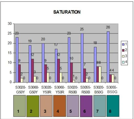
Figure 6.3. The Graph of Preference of Saturation for the Selected Colors, illuminated by the Created Light.

1 2 3 4 5 6 7 8 B50G

(27)

A t-test was conducted for the pairs of conditions. Similar to hue and brightness, the significance of the pairs including the second box was examined. All the pairs have significances below 0.05, except the 41st pair (Appendix G.3). In that pair, saturation of the seventh color, S3020-B50G, was evaluated under the conditions in the second box and the fourth box. The significance 0.451 reveals the fact that subjects had difficulty in evaluating the created light and the LED with 6500-Kelvin CCT. The color, S3020-B50G, is a blue dominant, turquoise-like color. The reason for the confusion of the subjects could be the blue-dominant spectral characteristics of the 6500-Kelvin LED in the fourth box.

Valuable data were gathered after the evaluation of the saturation of the colors under four lights results. Similar to the results of brightness, the first two color pairs, S3020-G50Y – G50Y and S3020-Y50R – S3060-Y50R, have significant differences than the last two color pairs, S3020-R50B – S3055-R50B and S3020-B50G – S3055-B50G. For the first two pairs, the preferences of the tints of the colors were more than their shades. The opposite result was obtained for the last two pairs (Figure 6.3)

(28)

In the seventh condition, 18 subjects (52.9%) preferred the created light (Table 5.24) while light in the final condition was preferred by 26 subjects (76.5%) (Table 5.25).

In all conditions, subjects continuously preferred the created light that reveals the saturation of the colors successfully.

Table 5.23. Saturation Frequency for Color: S3055-R50B, Light: Created Light S_6_2 25 73.5 73.5 73.5 7 20.6 20.6 94.1 2 5.9 5.9 100.0 34 100.0 100.0 1 2 3 Total Valid

Frequency Percent Valid Percent

Cumulative Percent

Table 5.24. Saturation Frequency for Color: S3020-B50G, Light: Created Light S_7_2 18 52.9 52.9 52.9 8 23.5 23.5 76.5 8 23.5 23.5 100.0 34 100.0 100.0 1 2 3 Total Valid

Cumulative Percent

Table 5.25. Saturation Frequency for Color: S3055-B50G, Light: Created Light S_8_2 26 76.5 76.5 76.5 4 11.8 11.8 88.2 4 11.8 11.8 100.0 34 100.0 100.0 1 2 3 Total Valid

Cumulative Percent

(29)

In the fourth condition, the saturation of S3060-Y50R was evaluated. 17 subjects (50%) preferred the created light, while 12 (35.3%) ranked it two and 5 subjects (14.7%) ranked it three (Table 5.21).

The fifth condition showed a significant preference of the created light. 23 subjects (67.6%) prefers that light and it was the second choice of only 10 subject (29.4%) (Table 5.22).

The saturation of the sixth color, S3055-R50B, was revealed successfully under the created light to 25 subjects (73.5%) (Table 5.23).

Table 5.21. Saturation Frequency for Color: S3060-Y50R, Light: Created Light S_4_2 17 50.0 50.0 50.0 12 35.3 35.3 85.3 5 14.7 14.7 100.0 34 100.0 100.0 1 2 3 Total Valid

Cumulative Percent

Table 5.22. Saturation Frequency for Color: S3020-R50B, Light: Created Light S_5_2 23 67.6 67.6 67.6 10 29.4 29.4 97.1 1 2.9 2.9 100.0 34 100.0 100.0 1 2 3 Total Valid

Cumulative Percent

(30)

The brightness of the second color was evaluated and 19 subjects (55.9%) preferred the created light, whereas 12 subjects (35.3%) gave a rank of two (Table 5.19).

The performance of the created light on the brightness of the third color, S3020-Y50R, was the first choice of 20 subjects (58.8%). Nine and five subjects (26.5% and 14.7%) gave a rank of two and three, respectively (Table 5.20).

Table 5.18. Saturation Frequency for Color: S3020-G50Y, Light: Created Light S_1_2 23 67.6 67.6 67.6 9 26.5 26.5 94.1 2 5.9 5.9 100.0 34 100.0 100.0 1 2 3 Total Valid

Cumulative Percent

Table 5.19. Saturation Frequency for Color: S3060-G50Y, Light: Created Light

S_2_2 19 55.9 55.9 55.9 12 35.3 35.3 91.2 3 8.8 8.8 100.0 34 100.0 100.0 1 2 3 Total Valid

Cumulative Percent

Table 5.20. Saturation Frequency for Color: S3020-Y50R, Light: Created Light S_3_2 20 58.8 58.8 58.8 9 26.5 26.5 85.3 5 14.7 14.7 100.0 34 100.0 100.0 1 2 3 Total Valid

Cumulative Percent

(31)

to the shades. However, the preference ranking data showed no certain relation between the tints and shades of any colors.

The first and fifth colors were preferred less than their shades, second and sixth colors. On the contrary, the third color was preferred more than its shade. For the case of colors S3020-B50G and S3055-B50G, the evaluations were equal. The preference rank of the fourth color, S3060-Y50R, had an outstanding result. The number of subjects, who ranked it one and two were same. This can be explained by the luminance of this color that is relatively low, when compared to other colors.

Although a certain relation cannot be observed in the data distribution, the brightness of the eight colors was preferred when compared to other light sources.

5.4. ANALYSIS OF PREFERENCE OF SATURATION

The subjects evaluated the appearances of the saturation of the eight colors. The results were statistically analyzed and frequency tables for each color with the created light was prepared. In the first condition, 23 subjects (67.6%) gave a rank of one, whereas 9 subjects (26.5%) gave a two and 2 subjects (5.9%) ranked it three (Table 5.18).

(32)

no certain relation between the tints and shades of the color pairs. However, the first four colors and the last four colors showed an unusual distribution of scores (Figure 6.2).

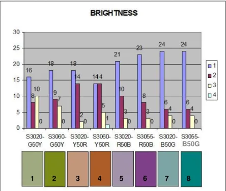
The distribution of the preference levels in the first four colors was below 20 subjects (58.8%). On the last four colors, it was the opposite. The subjects found the final four colors as the best light source, where as for the first four colors, they could not evaluate the colors clearly. Especially for the third and fourth colors, the ranks one and two were very similar.

In the data, gathered for the evaluation of brightness, Helmholtz-Kohlrausch effect would be expected to appear. This effect, explained in Chapter 3.3.2, hypothesized that; the tints of all colors should be preferred when compared

Figure 6.2. The Graph of Preference of Brightness for the Selected Colors, illuminated by the Created Light.

1 2 3 4 5 6 7 8 B50G

(33)

Except for the third and fourth conditions, the majority of the subjects found the created light to be the ideal light source that reveals the brightness of the colors successfully.

A t-test was conducted between the 48 pairs, to display the two-tailed probability of the difference. All the pairs, including the second box, have certain significances. Only the fifth and eleventh pairs showed significances of 0.615 and 0.065, respectively, that is, greater than 0.05 (Appendix G.2). In the case of the fifth pair, the object with S3020-G50Y color in the second box was compared with the same color in the fourth box. In the eleventh pair, the second box and the fourth box were compared to the color S3060-G50Y. The first color, S3020-G50Y, with the significance of 0.615, is the tint of the

second color having a significance of 0.065. The colossal significance, difference between these two pairs, is due to the brightness levels of the two colors.

The subjects evaluated the brightness of the color of the objects under the created light. The data gathered from their evaluation showed that the subjects preferred the created light. Unlike the evaluation of hue, there was

Table 5.17. Brightness Frequency for Color: S3055-B50G, Light: Created Light B_8_2 24 70.6 70.6 70.6 6 17.6 17.6 88.2 4 11.8 11.8 100.0 34 100.0 100.0 1 2 3 Total Valid

Cumulative Percent

(34)

The sixth condition showed a significant preference of the created light. 23 subjects (67.6%) ranked it one, whereas 8 and 3 ((23.5% and 8.8%) subjects ranked it two and three, respectively (Table 5.15).

In the seventh condition, 24 subjects (70.6%) found created light to be the ideal light source for the appearance of brightness of the object, painted with S3020-B50G (Table 5.16).

In the final condition, the same result was obtained, 24 subjects (70.6%) preferred the created light (Table 5.17).

Table 5.15. Brightness Frequency for Color: S3055-R50B, Light: Created Light B_6_2 23 67.6 67.6 67.6 8 23.5 23.5 91.2 3 8.8 8.8 100.0 34 100.0 100.0 1 2 3 Total Valid

Cumulative Percent

Table 5.16. Brightness Frequency for Color: S3020-B50G, Light: Created Light B_7_2 24 70.6 70.6 70.6 6 17.6 17.6 88.2 4 11.8 11.8 100.0 34 100.0 100.0 1 2 3 Total Valid

Cumulative Percent

(35)

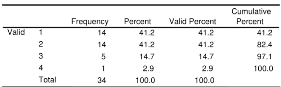
In the fourth condition, a similar result was obtained. The number of subjects (14 – 41.2%), who ranked it one, is the same as those, who ranked it two (Table 5.13).

The reason for these insignificant results may be the nature of the colors: S3020-Y50R and S3060-Y50R. These colors have red on the color composition of their surface. The subjects evaluated the colors under four lights, in comparison to the D65 illuminant that has dominant blue wavelength in its spectral distribution. It is clear that the appearance of a color with red pigments, under the reddish created light (with low CCT), will not appear same as it would under the bluish reference illuminant (with high CCT).

In the fifth condition, 21 subjects (61.8%) preferred the performance of the created light on the appearance of the brightness of the fifth color (Table 5.14).

Table 5.13. Brightness Frequency for Color: S3060-Y50R, Light: Created Light B_4_2 14 41.2 41.2 41.2 14 41.2 41.2 82.4 5 14.7 14.7 97.1 1 2.9 2.9 100.0 34 100.0 100.0 1 2 3 4 Total Valid

Cumulative Percent

Table 5.14. Brightness Frequency for Color: S3020-R50B, Light: Created Light B_5_2 21 61.8 61.8 61.8 10 29.4 29.4 91.2 1 2 Valid

Cumulative Percent

(36)

In the second condition, in which the subjects were evaluating the brightness of the object, painted with the second color (S3060-G50Y), 18 subjects (52.9%) found the created light to be the best light source (Table 5.11)

Different from the other conditions, mentioned above, the third condition showed only a minor significance between the preference levels of the subjects. In this condition, 18 subjects (52.9%) gave a rank of one, whereas 14 subjects (41.2%) gave a rank of two. Although the number of subjects, whose first choice was the created light, is greater than those who put the created light into second position, the majority of the subjects preferred the created light (Table 5.12).

Table 5.11. Brightness Frequency for Color: S3060-G50Y, Light: Created Light B_2_2 18 52.9 52.9 52.9 9 26.5 26.5 79.4 7 20.6 20.6 100.0 34 100.0 100.0 1 2 3 Total Valid

Cumulative Percent

Table 5.12. Brightness Frequency for Color: S3020-Y50R, Light: Created Light B_3_2 18 52.9 52.9 52.9 14 41.2 41.2 94.1 2 5.9 5.9 100.0 34 100.0 100.0 1 2 3 Total Valid

Cumulative Percent

(37)

like the others, were evaluated under D65 illuminant for reference. This illuminant, with its blue-dominant spectral distribution characteristics, rendered the colors S3020-R50B and S3055-R50B different than the other pairs. The opposite of the Abney effect occurred for this case due to this fact.

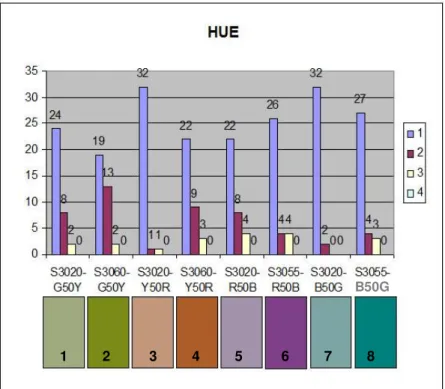
For all the cases, 20 subjects (58.8%) that is more than half of the sample group, ranked the created light as the first choice. This showed that, the hue of the colors appeared more attractive for the observers, when illuminated with the light that had the same CC with the object.

5.3. ANALYSIS OF PREFERENCE OF BRIGHTNESS

The responses of the subjects for the preference of the brightness of colors under the four lights were examined. In the first condition, 16 subjects (47.1%) preferred the created light, while 8 subjects (23.5%) gave a rank of two and 10 subjects (29.4%) gave a rank of three, for the appearance of the first color under the created light (Table 5.10).

Table 5.10. Brightness Frequency for Color: S3020-G50Y, Light: Created Light B_1_2 16 47.1 47.1 47.1 8 23.5 23.5 70.6 10 29.4 29.4 100.0 34 100.0 100.0 1 2 3 Total Valid

Cumulative Percent

(38)

The data gathered in this dissertation showed that the hues of the objects were preferred more, when illuminated with the created light, compared to other conventional lights. In Figure 5.1, the graphical presentation of the data shows the preference distribution of the subjects for the colors.

There is a visible relation between the tint and shade tones of the color pairs. For the six colors, except the fifth and sixth colors, the tints of the colors are preferred more than their shades. This can be explained by the Abney effect, explained in Chapter 3.3.1. When white is added to the color, a shift in hue occurs and when comparing the two pairs, the tint of a color is preferred more than its shade. In the case of the color pairs, S3020-R50B and S3055-R50B, shades were preferred more than their tints. This can be explained by the blue-dominant spectral composition of the color itself. These color pairs,

Figure 5.1. The Graph of Preference of Hue for the Selected Colors, illuminated by the Created Light.

1 2 3 4 5 6 7 8 B50G

(39)

In all eight cases, none of the subjects found the appearance of the hue under the created light to be poor and gave a rank of four and for those eight specific conditions. The majority of the observers preferred the appearance of the hue of the objects under the created light.

The individual evaluations for the eight colors identified the preference of the subjects for each condition. However, the conditions were matched as pairs and a t-test was conducted between those 48 pairs, to display the two-tailed probability of the difference between the means (Appendix G.1). The t-test calculates whether the means of two groups are statistically different from each other.

The evaluation results of the pairs are statistically significant, if the

significance is below 0.05. If the value is greater than 0.05, then there is not enough evidence to state a difference. Although the paired sample tests for hue showed 48 significance values, the pairs including the second box14 were more valuable for the study. Among those 24 pairs, including the

second box, only two of them (Pair 11 – 0.061 and Pair 29 – 0.148) showed a significance value that is greater than 0.05 (Appendix G.1, Table G.1), in the boxes with the created light and the LED sources with a CCT of 6500 Kelvin, for the colors S3060-G50Y and S3020-R50B. The reason for not having a significant difference between the appearances of the hue of the colors under these two lights may be the difficulty of differentiating the appearance of the colors between the created light and 6500 K light for these special cases.

(40)

26 subjects (76.5%) preferred the created light in the sixth condition, while four subjects (11.85%) only as the second rank (Table 5.7).

In the seventh condition, a remarkable result was obtained. 32 subjects (94.1%) preferred the appearance of the hue of S3020-B50G under the created light. Only two subjects (5.9%) gave a rank of two (Table 5.8).

The preference ratio of the created light in the last condition was not different from the others. 27 subjects (79.4%) gave a rank of one for the created light (Table 5.9).

Table 5.7. Hue Frequency for Color: S3055-R50B, Light: Created Light H_6_2 26 76.5 76.5 76.5 4 11.8 11.8 88.2 4 11.8 11.8 100.0 34 100.0 100.0 1 2 3 Total Valid

Cumulative Percent

Table 5.8. Hue Frequency for Color: S3020-B50G, Light: Created Light H_7_2 32 94.1 94.1 94.1 2 5.9 5.9 100.0 34 100.0 100.0 1 2 Total Valid

Cumulative Percent H_8_2 27 79.4 79.4 79.4 4 11.8 11.8 91.2 3 8.8 8.8 100.0 34 100.0 100.0 1 2 3 Total Valid

Cumulative Percent Table 5.9. Hue Frequency for Color: S3055-B50G, Light: Created Light

(41)

The fourth condition, for the object painted with S3060-Y50R, 22 subjects (64.7%) preferred the appearance under the created light, while nine subjects (26.5%) gave a rank of two, and three subjects (8.8%) gave a rank of three (Table 5.5).

For the evaluation of the fifth condition, 22 subjects (64.7%) chose the created light as the best light source among the other three light sources in the case of appearance of the hue (Table 5.6).

Table 5.4. Hue Frequency for Color: S3020-Y50R, Light: Created Light H_3_2 32 94.1 94.1 94.1 1 2.9 2.9 97.1 1 2.9 2.9 100.0 34 100.0 100.0 1 2 3 Total Valid

Cumulative Percent

Table 5.5. Hue Frequency for Color: S3060-Y50R, Light: Created Light H_4_2 22 64.7 64.7 64.7 9 26.5 26.5 91.2 3 8.8 8.8 100.0 34 100.0 100.0 1 2 3 Total Valid

Cumulative Percent

Table 5.6. Hue Frequency for Color: S3020-R50B, Light: Created Light H_5_2 22 64.7 64.7 64.7 8 23.5 23.5 88.2 4 11.8 11.8 100.0 34 100.0 100.0 1 2 3 Total Valid

Cumulative Percent

(42)

created light. Eight subjects (23.5%) gave a rank of two and two subjects (5.9%) gave a rank of three (Table 5.2).

In the second condition, for the object with S3060-G50Y paint, 19 subjects (55.9%) preferred the created light, 13 subjects (38.2%) rated the revealing of the appearance of hue under the created light into the second place, whereas only two subjects (5.9%) recorded a rank of three (Table 5.3).

The third condition showed a remarkable preference difference among the subjects. 32 subjects (94.1%) preferred the appearance of the objects under the created light (Table 5.4).

Table 5.3. Hue Frequency for Color: S3060-G50Y, Light: Created Light H_2_2 19 55.9 55.9 55.9 13 38.2 38.2 94.1 2 5.9 5.9 100.0 34 100.0 100.0 1 2 3 Total Valid

Cumulative Percent Table 5.2. Hue Frequency for Color: S3020-G50Y, Light: Created Light

H_1_2 24 70.6 70.6 70.6 8 23.5 23.5 94.1 2 5.9 5.9 100.0 34 100.0 100.0 1 2 3 Total Valid

Cumulative Percent

(43)

their responses. A Cronbach’s Alpha value of 0.969 was obtained from the test group, after excluding five subjects (Table 5.1.).

Cronbach's Alpha

N of Items

,969 34

The widely accepted cut-off for Cronbach’s alpha in social sciences “should be 0.80 or higher for a set of items to be considered to have an observer accuracy” (Garson, n.d., sect. Cronbach’s Alpha, para. 4). The responses of the remaining 34 “statistically reliable” subjects were investigated for the dissertation.

5.2. ANALYSIS OF PREFERENCE OF HUE

The responses of the subjects, for the eight colors under the illuminance of four different lights, were statistically analyzed. For each condition, a

frequency table was prepared. Although all the data is valuable for the study to a certain degree, the conditions for the created light, however, was more important than the other conditions with 3000, 4200 and 6500 K light sources. Eight tables among 32 tables were chosen with this concern to evaluate the response of the observers.

In the first condition, 24 of 34 subjects (70.6% of the subject group) preferred the appearance of the hue of the object with S3020-G50Y paint, under the

(44)

5. DATA ANALYSIS OF THE EXPERIMENTAL STUDY

The results of the experiment were transferred into a computer as data sets. These sets were statistically investigated by using the SPSS software, Version 14. SPSS is the abbreviation of “Statistical Package for the Social Sciences” and it is widely used by more than 90% of the universities in the United States (About SPSS, n.d.).

5.1. ANALYSIS OF THE RELIABILITY OF THE SUBJECTS

Reliability is the correlation of an item, scale, or instrument with a

hypothetical one that truly measures what it is supposed to (Garson, n.d.). When the true instrument is not available, reliability can be estimated by certain methods. One of the most common is the “inter-rater reliability test”. It is based on the correlation of scores between two or more raters who rate the same item, scale or instrument. “Cronbach’s alpha” or the “reliability coefficient” is the most common form of reliability coefficient for the internal consistency, based on average correlation among items.

The experiment was initially conducted with 39 subjects. To evaluate the reliability of the subject responses, an inter-rater reliability test was applied to

(45)

appearance of the objects in each box from one to four, compared to the object in the reference box. Before each evaluation process, the definitions of hue, brightness, and saturation were read aloud from a text. By defining the terms, the subjects became aware of the evaluation criteria and possible confusions were omitted.

The box with a “point one” means, “it is the box that successfully illuminates the object that has the same or closest appearance as if it is in the reference box”. The “point four” means farthest.

The objects were located at the center of each box and the subjects were asked to fill out the survey leaflet. For each experiment phase, the created light was changed when the subjects completed their evaluation of the specified color (see Appendix E for the photographs of each scene for each color).

(46)

Due to the tripled nature of the RGB mixture method, measurement devices cannot calculate the photometric properties of the total radiation directly, since there are three different sources emitting light of different ratios. In that case, indirect measurement of the light reflected from a Barium Sulfate13 coated surface provides the correct results.

4.4. THE PROCEDURE OF THE EXPERIMENT

The experiment was conducted for three days and only one subject was tested at a time. The average test duration was approximately 20 minutes. To test whether the subjects had any ophthalmologic problems, a color

blindness test was conducted with pseudoisochromatic plates. Any kind of eye deficiency or color blindness of a subject would effect the perception of colors under different lights. To prevent any possible bias, the four boxes were shuffled, so that the subjects were not aware of any changes in one box in a constant position (see the Table 3.3: Shuffling Order of the Experiment Boxes on Page 60). The subjects were asked to turn their backs, while the boxes are shuffling. On the other hand, they were informed that all the five objects were painted with the same color. Each subject had eight survey leaflets, prepared specially for the colors they were going to evaluate. A sample survey leaflet can be found on Appendix F. On each leaflet, there were questions that were aimed to be evaluated by the three standard attributes of visual sensation: hue, brightness, and saturation. Each subject was asked to evaluate these three criteria for each color, by ranking the

13_{Barium Sulfate is a diffuse white reflective coating that offers greater than 97% reflectance between 450 and} 900nm.

(47)

In the laboratory, the CS100 and DP101 were connected and the created lights were measured. As seen in Figure 4.20, the devices were measuring a light, created by some LED clusters.

The Calibration Palette

The light measuring devices can measure light by direct or indirect method. The direct method measures the photometric properties of light directly from the light source, whereas the indirect method measures the reflected light from a reflective surface. In some cases, the direct method cannot be useful, since the light level of the source can extend to the upper limit of the lighting measurement device.

Figure 4.19. The DP101 Data Processor

(48)

The luminance and chromaticity calculations of color televisions and CRTs, projection equipments and video projectors can be conducted by using this device.

A CS 100 Chromameter from Minolta, serial number of 19013037, was used to control and measure the created lights. The device gives two major data: the illuminance and Chromaticity Coordinates. (Figure 4.18)

The Data Processor

By using the Data Processor (DP-101), measured values can be calculated in terms of Yxy, L*a*b*, Color Temperature, and Correlated Color

Temperature as the distance from blackbody locus ∆uv for absolute color values. DP-101 has memory space for up to 300 sets of measurement data and a built-in thermal printer for printing out data, either at the time of

measurement or from memory at a later time. In the experiment, the DP-101 with a serial number 331064 was used for data storage and printouts (Figure 4.19).

(49)

The surface color of an object can be measured by a spectrophotometer in few seconds and CC values are obtained simultaneously. These coordinates can be kept in computers that are attached to the device or printed out as a hardcopy. Every spectrophotometer measures the CC values of object and if desired, the output can be converted into other standard color spaces.

The Chromameter

The CS 100 Chromameter is used for measuring the Chromaticity

Coordinates and luminance of the light sources and surfaces. It can measure luminance and chromaticity of small light sources, such as LEDs or miniature neon lamps. It can also be useful for measuring luminance and chromaticity of general light sources, such as tungsten lamps or fluorescent lamps. This device is widely used in calibrating the luminance and chromaticity of traffic signals and emergency exit lamps. The Chromameter is useful for reflective subject measurements of objects that cannot be measured by contact methods, such as distant building walls, painted surfaces, subjects with complicated shapes, or surfaces that should not be touched for sanitary

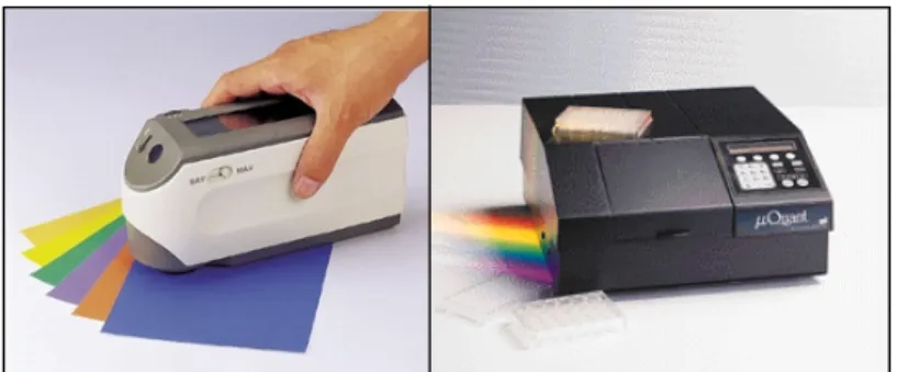
Figure 4.17. Two Examples for Spectrophotmeters, Konica Minolta CM-2600D, and µQuantTM Universal Microplate Spectrophotometer.

(50)

They were young subjects, having healthy vision and an architectural

education of a certain level. 74% of the students had courses related to color in their education, while 26% of the subjects worked with primary colors in their first year students.

Before the test, they were asked about visual defects. Subjects with eye deficiency were asked to use their correction equipments, like glasses and lenses. Also, their color discrimination and vision abilities were tested before the experiment by pseudoisochromatic plates.

4.3.3. THE CONTROL DEVICES

The Spectrophotometer

The conversion tables and programs determined the CC values of the objects in the experiment. However, working with genuine museum artifacts, it is not possible to have color-notated objects. In that case a

spectrophotometer can measure the CC of the surface of the object. By using such a device, the color of a specimen can be measured according to a variety of standards12 like XYZ, L*a*b*, RGB, CMYK, and Yxy. There are portable and tabletop type spectrophotometers, like the ones shown in Figure 4.17. Museums can afford to buy them for their laboratories, or they can borrow from other institutions. In some cases, other museum laboratories could help them and answer their needs.

12_{Like CIE 1931 Yxy color space, the XYZ, L*a*b*, RGB, and CMYK are different kinds of color spaces that were} out of scope of this study.

(51)

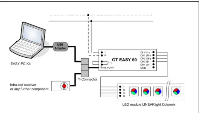
DALI system, designed for the experiment, are drawn schematically in Figure 4.15.

4.3.2. THE SUBJECTS

The experiment was conducted with 34 university students. The gender distribution of the subjects is 19 female and 15 male subjects, having an average age of 21,08. Majority of the subjects (44%) were 21 years old and 59% of them were second year students. Figure 4.16 shows the detailed presentation of the age group and class of the subjects in percentage.

Figure 4.15. A Schematic Drawing of the DALI System Created in the Experiment. CLASS 26% 59% 15% 0% 1 2 3 4 AGE 9% 12% 44% 32% 3% 19 20 21 22 23

(52)

The DALI System

In the DALI systems, the software for a dynamic color control controls the intensities of red, green, and blue LEDs individually. By using this software, intensity of each LED can be increased or decreased. The CC of the white light can be measured by using a chromameter that measures the

photometric properties of the light source. Increasing or decreasing the intensities of the red, green and blue LEDs should be done by a

computerized system. In this study, an experiment was conducted previously, by using manual dimmers. However, imprecise CC values were obtained with difficulty after numerous attempts. This experience showed the necessity of a computerized system. A DALI system, based on computers and precise adjustments of the light levels of each LED, increased the reliability of the experiments.

To create the desired lights, The EasyColor Control software and DALI systems of OSRAM were used. The screenshot of the EasyColor Control is shown in Figure 4.1, on page 44. The software was installed on a computer with Intel Pentium IV 3.06 MHz processor and 512 MB RAM memory.

The main device of the DALI system from OSRAM was OT Easy 60. Its initial purpose was to connect the computer with the LED clusters. The second purpose was to provide an electric current for the DALI circuit. The

(53)

The shuffling order of the boxes for the eight colors is listed in Table 3.3.

Color Number

NCS

Notation Shuffling Order

1st Box 2nd Box 3rd Box 4th Box

1 S3020-G50Y B3 BD B4 B6 2 S3060-G50Y B3 B4 BD B6 3 S3020-Y50R B3 B4 B6 BD 4 S3060-Y50R BD B4 B6 B3 5 S3020-R50B B3 BD B4 B6 6 S3055-R50B B3 B4 BD B6 7 S3020-B50G B3 B4 B6 BD 8 S3055-B50G BD B4 B6 B3

B3: The box with the 3000 K LED B4: The box with the 4200 K LED B6: The box with the 6500 K LED

BD: The box with the Desired CC

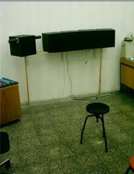
Figure 4.14 shows a photograph of the experimental setup. The boxes and the sitting position of the subjects were carefully adjusted.

Table 3.3. The Chosen Colors and the Shuffling order of the Experiment Boxes

(54)

in the experiment. These delicate palettes are used to measure the

photometric properties of the light sources. By using the small pegs on the slanted surface, the palettes were securely fixed. In Figure 4.11 and 4.12, the slanted surfaces can be seen.

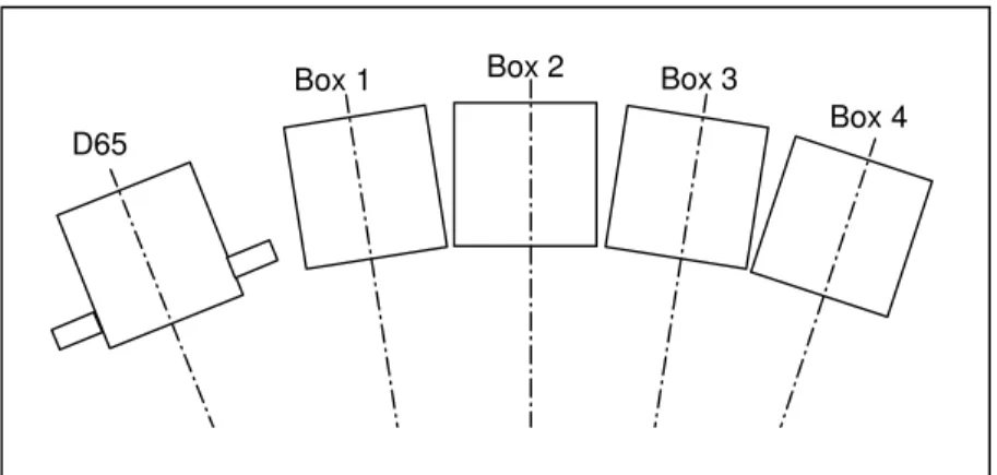
The five boxes were located with a polar array, to provide equal lines of sight for the subjects. The schematic drawing of this layout can be seen in the plan drawing of the experiment room in Figure 4.8. Each spherical object and box had identical visual conditions. The reference box on the left, containing the D65, was separated by 10 cm from the other four boxes. The electric cable layout was designed to be flexible, to allow shuffling the boxes. The box with the created light should be methodically shuffled with other three boxes with 3000, 4200, and 6500 K LEDs, to reduce any possible bias of the subjects (Figure 4.13).

Figure 4.13. The Schematic Drawing of Five Boxes. D65

Box 1 Box 3

Box 4

(55)

identical boxes, and if the reference box were wider than the other four boxes, than the subjects would be biased. On the other hand, if all the five boxes were of 65 cm width, then the total experimental setup would need to be at least 325 cm long. This would exceed the cone of vision of the subjects. The solution was to fulfill the requirements of the experiment by modifying the fifth box. Two holes with, 5 cm diameter, were drilled on both sides of the boxes. The two ends of the fluorescent tubes protruded from the box. To avoid direct glare and hide the unwanted light outside the box, plastic tubes were applied to two edges of both. In Figure 4.12, the technical drawing of the reference box is shown.

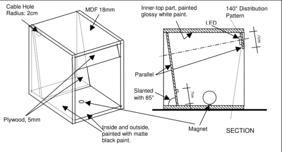
The backgrounds of the boxes were slanted at 85 degrees. There were two reasons for this. The first was to provide a better inter-reflection of the light rays, coming from the LEDs that were also fixed on the slanted surfaces. The background of the boxes and the LED bases were parallel to each other. The

Figure 4.12. The Technical Drawing of the Reference Box.

7

c

m

Inner-top part, painted glossy white paint.

SECTION MDF, 18mm Magnet Parallel 7 c m D65

Plastic tube with 5cm Radius

Slanted with 85°

Inside and outside, painted with matte black paint. Plywood, 5mm

Cable Hole Radius: 2cm