Parafac-spark: parallel tensor decompositions on spark

PARAFAC-SPARK: PARALLEL TENSOR

DECOMPOSITIONS ON SPARK

a thesis submitted to

the graduate school of engineering and science

of bilkent university

in partial fulfillment of the requirements for

the degree of

master of science

in

computer engineering

By

Selim Eren Bek¸ce

August 2019

PARAFAC-SPARK: Parallel Tensor Decompositions on Spark By Selim Eren Bek¸ce

August 2019

We certify that we have read this thesis and that in our opinion it is fully adequate, in scope and in quality, as a thesis for the degree of Master of Science.

Cevdet Aykanat(Advisor)

Muhammet Mustafa ¨Ozdal(Co-Advisor)

Halil Altay G¨uvenir

Fahreddin S¸¨ukr¨u Torun

Approved for the Graduate School of Engineering and Science:

Ezhan Kara¸san

ABSTRACT

PARAFAC-SPARK: PARALLEL TENSOR

DECOMPOSITIONS ON SPARK

Selim Eren Bek¸ce M.S. in Computer Engineering

Advisor: Cevdet Aykanat

Co-Advisor: Muhammet Mustafa ¨Ozdal August 2019

Tensors are higher order matrices, widely used in many data science appli-cations and scientific disciplines. The Canonical Polyadic Decomposition (also known as CPD/PARAFAC) is a widely adopted tensor factorization to discover and extract latent features of tensors usually applied via alternating squares (ALS) method. Developing efficient parallelization methods of PARAFAC on commodity clusters is important because as common tensor sizes reach billions of nonzeros, a naive implementation would require infeasibly huge intermediate memory sizes. Implementations of PARAFAC-ALS on shared and distributed-memory systems are available, but these systems require expensive cluster setups, are too low level, not compatible with modern tooling and not fault tolerant by design. Many companies and data science communities widely prefer Apache Spark, a modern distributed computing framework with in-memory caching, and Hadoop ecosystem of tools for their ease of use, compatibility, ability to run on commodity hardware and fault tolerance. We developed PARAFAC-SPARK, an efficient, parallel, open-source implementation of PARAFAC on Spark, written in Scala. It can decompose 3D tensors stored in common coordinate format in parallel with low memory footprint by partitioning them as grids and utilizing compressed sparse rows (CSR) format for efficient traversals. We followed and combined many of the algorithmic and methodological improvements of its pre-decessor implementations on Hadoop and distributed memory, and adapted them for Spark. During the kernel MTTKRP operation, by applying a multi-way dy-namic partitioning scheme, we were also able to increase the number of reducers to be on par with the number of cores to achieve better utilization and reduced memory footprint. We ran PARAFAC-SPARK with some real world tensors and evaluated the effectiveness of each improvement as a series of variants compared

iv

with each other, as well as with some synthetically generated tensors up to bil-lions of rows to measure its scalability. Our fastest variant (PS-CSRSX ) is up to 67% faster than our baseline Spark implementation (PS-COO ) and up to 10 times faster than the state of art Hadoop implementations.

Keywords: spark, tensor, factorization, decomposition, parafac, cpd, als, alter-nating squares, parafac-als, cpd-als, hadoop, grid, partitioning, data science, big data.

¨

OZET

PARAFAC-SPARK: SPARK ˙ILE PARALEL TENS ¨

OR

AYRIS

¸IMLARI

Selim Eren Bek¸ce

Bilgisayar M¨uhendisli˘gi, Y¨uksek Lisans Tez Danı¸smanı: Cevdet Aykanat

˙Ikinci Tez Danı¸smanı: Muhammet Mustafa ¨Ozdal A˘gustos 2019

Tens¨orler veri bilimi uygulamalarında ve bilimsel ¸calı¸smalarda sık¸ca kul-lanılmakta olan ¸cok boyutlu matrislere verilen isimdir. Paralel Fakt¨or Analizi (PARAFAC) adıyla bilinen ayrı¸sım ¸sekli, yaygın olarak kullanılan alternatif k¨okler (ALS) tens¨or ayrı¸stırma algoritması sayesinde veri ¨uzerindeki ¨ort¨uk ¨ozellikler ve fakt¨or matrisleri ortaya ¸cıkarabilmektedir. G¨un¨um¨uzde geli¸smi¸s teknolojiler ve b¨uy¨uk veri biliminin yaygınla¸smasıyla birlikte ortaya ¸cıkan tens¨orler milyarlarca satır veri i¸cerebilmektedir. Bu algoritmanın basit bir uygulaması ¸cok b¨uy¨uk boyutlarda ara matris ve veri ileti¸simi gerektirdi˘ginden, paralel sistemlerde etkin bir bi¸cimde uygulanabilmesi, b¨uy¨uk veri biliminin geli¸simi i¸cin ¨onem kazanmak-tadır. PARAFAC-ALS’in payla¸sımlı veya da˘gıtık bellekli sistemlerde uygula-maları mevcuttur fakat bu sistemler maliyetli sistem yatırımları ve d¨u¸s¨uk se-viye kodlama gerektirir, ¸ca˘gda¸s programlama ara¸clarıyla uyumsuzdur ve ola˘gan sistem ve altyapı arızalarına dayanıklı da de˘gillerdir. Apache Spark ¨onbellek destekli ¸ca˘gda¸s ve da˘gıtık bir programlama platformudur ve Apache Hadoop eko-sistemi ile birlikte bir¸cok ¸sirket ve veri bilimcisi tarafından uyumlu, ekonomik ve hataya dayanıklı olmaları sebebiyle tercih edilmektedir. Spark ¨uzerinde Scala diliyle geli¸stirdi˘gimiz paralel PARAFAC-SPARK uygulaması, ¨u¸c boyutlu tens¨orleri d¨u¸s¨uk bellek t¨uketimiyle ayrı¸stırabilmektedir. ˙I¸slem sırasında tens¨orler daha hızlı ve da˘gıtık ¸sekilde i¸slenebilmeleri i¸cin sıkı¸stırılmı¸s seyrek satırlar (CSR) formatına d¨on¨u¸st¨ur¨ul¨ur ve tens¨or k¨up ¸seklinde par¸calara ayırılıp da˘gıtılarak i¸slenir. Bu ¸calı¸smada, ¨onceki da˘gıtık bellek ve Hadoop uygulamalarındaki algo-ritmik ve y¨ontemsel geli¸stirmeler derlenip en uygun ¸sekilde Spark i¸cin yeniden uyarlanmı¸stır. Ayrıca, ana Matrisle¸stirilmi¸s Tens¨or ile Khatri-Rao C¸ arpımı (MTTKRP) operasyonu sırasında ¸cok boyutlu dinamik payla¸stırma tekni˘gi uygulanmı¸s, bu sayede MTTKRP operasyonunun bellek t¨uketiminde dinamik

vi

payla¸stırma katsayısı oranında azalma ve operasyonun son indirgeme a¸samasında da i¸slemci kapasite kullanım oranında artma sa˘glanmı¸stır. PARAFAC-SPARK uygulamasını 11 ger¸cek veri i¸ceren tens¨or ve ¨ol¸ceklenebilirli˘gi test etmek adına sentetik olarak ¨uretilmi¸s tens¨orler i¸cin ¸calı¸stırdık. En ileri varyasyonumuzun (PS-CSRSX ), temel Spark varyasyonuna (PS-COO ) g¨ore %67’e kadar daha hızlı oldu˘gunu ve en ileri Hadoop uygulamalarına g¨ore 10 kata kadar daha hızlı oldu˘gunu g¨ord¨uk.

Anahtar s¨ozc¨ukler : spark, tens¨or, ayrı¸sım, fakt¨orizasyon, parafac, cpd, alternatif k¨okler, parafac-als, cpd-als, hadoop, grid, b¨ol¨umleme, veri bilimi, b¨uy¨uk veri.

Acknowledgement

To my professors Cevdet Aykanat and Mustafa ¨Ozdal, I am grateful for your valuable and constructive suggestions and criticism during this research work, thank you for everything.

To my grandfather, an honest, strong, diligent, generous, loving, passionate and modest man, he who always supported me during my studies and endeavors, called me “my professor”, showed us how to live in peace and harmony by sharing his unbounded love and unfolding his life’s stories in humbleness; you are with us now and we will always remember and love you, rest in peace.

To my beloved wife, mother, father and sister for loving, supporting and en-couraging me through my studies; this accomplishment would not have been possible without you, I love you all.

Contents

CONTENTS ix 2.3.3 Persistence . . . 20 2.3.4 Executor Settings . . . 21 2.4 Prior Art . . . 22 3 Methods 24 3.1 RDD Representations . . . 24 3.2 MTTKRP . . . 26

3.3 Caching & Reordering of Computations . . . 28

3.4 Dense Form Factor Matrices (DFFM) . . . 29

3.5 Grid Partitioning . . . 32

3.6 Compressed Sparse Row (CSR) Processing . . . 37

3.7 Multi-Mode Partitioning . . . 41 3.8 TrMM . . . 43 3.9 DstMM . . . 46 3.10 NormC . . . 47 4 Evaluation 49 4.1 Variants . . . 50

4.2 Setup and Parameter Tuning . . . 50

CONTENTS x

4.3.1 Real-World Tensor Runtime Experiment . . . 52 4.3.2 Data Scalability Experiment . . . 56

List of Figures

2.1 A three dimensional tensor . . . 5

2.2 MTTKRP Operation, Naive . . . 14

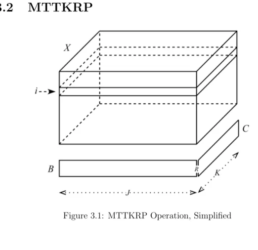
3.1 MTTKRP Operation, Simplified . . . 26

3.2 Grid partitioning . . . 33

3.3 Multi-Mode Partitioning (Partition Stretching) . . . 41

3.4 TrMM Operation . . . 44

4.1 Bar charts that show the iteration and total runtime values of gowalla, facebook-rm, movies-amazon, brightkite, food and NELL-2 datasets for Real-World Tensor Runtime Experiment including results of all variants. . . 53 4.2 Bar charts that show the iteration and total runtime values of

NELL-1, enron-3, flickr-3, yelp and delicious datasets for Real-World Tensor Runtime Experiment including results of all variants. 54 4.3 Data scalability experiment results that show the correlation

LIST OF FIGURES xii

4.4 Data scalability experiment results that show the correlation be-tween Mode Length (I=J=K) vs Runtime, where nnz = 10 × I. . 57

List of Tables

2.1 Transformation Operations . . . 18

2.2 Action Operations . . . 19

2.3 Storage Levels in Spark . . . 21

3.1 CSR Forms . . . 40

3.2 CSR Form Selection of Factor Matrices . . . 40

4.1 PARAFAC-SPARK variants . . . 50

4.2 List of the real-world input tensors that were used for evaluation of all variants with their mode lengths and non-zero counts. . . . 52 4.3 Full combined list of all iteration and total runtime results for

Chapter 1

Introduction

Tensors are the generalization of matrices into higher dimensions. They are widely used in data science where each dimension models specific attributes, e.g., cus-tomers, products, movies, interests, ratings, dates, measurements, etc. Such tensors may have billions of non-zeros. To understand the underlying proper-ties of the data well, various techniques like Tensor Decomposition are exercised. Canonical Polyadic Decomposition (CPD) is one form of Tensor Decomposition which can decompose tensors into lower rank tensors (factor matrices) that allows understanding critical relationships between its elements to be further utilized by data scientists.

PARAFAC-ALS is an algorithm for finding the CPD of an input tensor by utilizing Alternating Least Squares method. It finds core factor matrices which can represent the original tensor with least error. However, the key problem with PARAFAC-ALS is that a naive implementation becomes extremely inefficient due to the huge sizes of the intermediate matrices that need to be materialized during the kernel operation. Therefore the problem needs to be solved progressively in such a way that those intermediary matrices would not need to be materialized even in a distributed setting. This is an interesting property and the key challeng-ing feature of the several remarkable distributed tensor factorization solutions in

distributed and/or shared memory systems such as [1, 2]. Although these sys-tems are historically very popular due to the ability of low-level high-performance parallel programming interfaces, those systems often have high setup and main-tenance costs, too low level, not fault tolerant by design and incompatible with popular frameworks and infrastructures used by real-world data scientists.

In this work, we implement a fast and effective tensor decomposition solution on Apache Spark, which is a high-level distributed computing framework, for its built-in fault tolerance, compatibility with Apache Hadoop and popularity among the business world and data science professionals for its integrative ecosystem. Since there are no existing tools for this task in Spark, we will first examine existing solutions on Hadoop’s MapReduce and build a tangible baseline imple-mentation of PARAFAC-ALS on Spark that solves the key kernel optimization problem via progressively calculating the intermediaries without fully material-izing them, which also performs strictly better than Hadoop counterparts like [3, 4, 5]. This baseline will be our building point for the next phase of opti-mizations; Reordering of Computations, Caching, Grid Partitioning, Compressed Sparse Row (CSR) Format processing and Multi-Mode Partitioning, which are explained in detail in Chapter 3. Each of these optimizations has some param-eters to control their behavior, therefore during our experiments, we will adjust these variables then run different runtime measurements. We will name our im-plementation PARAFAC-SPARK.

Chapter 2 gives detailed preliminary information on tensors, their notation, representation, storage methods; definitions and examples of matrix operations used in PARAFAC-ALS, Canonical Polyadic Decomposition (CPD) and its ap-plications; PARAFAC-ALS algorithm itself and the motivation behind its par-allelization. This chapter also introduces Apache Spark, explains its working principles and Resilient Distributed Datasets (RDDs), lists its core operations used in the main phases of PARAFAC-SPARK and its partitioning and persis-tence features. This is important to understand the improvements suggested in the subsequent chapter.

at its core level. It first starts with how tensors and matrices used in PARAFAC-ALS will be represented as RDDs in Spark context, then moves on to describe the key implementation steps of MTTKRP such as Caching, Factor Matrices, Grid Partitioning, CSR Processing and Multi-Mode Partitioning. It then completes the PARAFAC-SPARK definition by describing Spark implementations of all sub-algorithms TrMM, DstMM and NormC with their runtime complexities to mark the end of the chapter.

Chapter 4 starts with explaining the runtime setup, evaluation criteria, methodology and experiments performed including the properties of real-world tensors that were used for evaluation. It then gives the experimental results and includes discussion on those results.

Chapter 5 concludes this work by summarizing achievements and discussion on future work.

Chapter 2

Preliminaries

2.1

Tensors

2.1.1

Definition

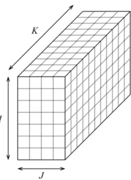
Tensors are multi-dimensional arrays. A vector is a one-dimensional tensor, and a matrix is a two dimensional one and the word tensor is generally used for higher dimensional arrays. Three-dimensional tensors can be visualized as a cube (Figure 2.1).

Tensors of three or more dimensions are increasingly found in many applica-tions, such as an e-commerce website constructing a three-mode tensor with users, products, and dates of purchase. Such tensor can be utilized in a recommendation or analysis system to derive metrics for the company. Another example tensor is generated sensor data, in which the first dimension represents the units, the second one represents the sensor identifier, and the third is the time of occur-rence. Such tensors can be huge; it is typical for an e-commerce website having hundreds of thousands of users and millions of products.

Figure 2.1: A three dimensional tensor

2.1.2

Representations

Vectors are represented with lowercase letters, e.g., a. Matrices are represented with uppercase letters, e.g., B. Tensors of three or more dimensions are repre-sented with uppercase calligraphic fonts, e.g., X .

Elements of tensors are denoted with indices inside square brackets. The ith element of vector a is denoted as a[i]. The element on indices (i, j) of matrix A is denoted as A[i, j]. The element on indices (i, j, k) of three-mode tensor X is denoted as X [i, j, k] and so on.

The number of dimensions of a tensor is called order or mode of the ten-sor. Index of each dimension start from 0 and increase until the length of that dimension, e.g., i = 0, . . . , I − 1.

A fiber is a vector obtained from fixing all but one dimension of an input tensor, e.g., each row and column of a matrix is a fiber. Fixed indices are denoted with non-negative integers or variables of same sort, whereas a colon character (:) represents a free index, e.g., X [i, j, :] means the first two indices are fixed and the third is free. For example, M [2, :] denotes the second row of matrix M .

A slice is a matrix obtained from fixing all but two dimensions of an input tensor, e.g., each horizontal plane of a three-order tensor is a slice. For example, X [:, :, 3] denotes the matrix in the third plane of tensor X .

Higher order tensors are typically unfolded to lower dimensions before apply-ing some mathematical operations on them. An N -dimensional tensor can be unfolded (or flattened ) into N tensors of N − 1 dimensions. Unfolding a three-mode tensor into a matrix is also called matricization. For example, let X be a three-dimensional tensor with size I ×J ×K. X(1)_{, X}(2)_{, X}(3)_{are three unfoldings}

of sizes I × J K, J × IK, K × IJ , respectively. The unfolding operation is applied with following method; to obtain X(i), traverse ith dimension of X by looping through next dimension in line each time the boundary of the current dimension is reached.

Example: Let X be a 2 × 3 × 3 tensor. Each plane (slices of third dimension) is seperated with |, respectively.

X = " 0 1 7 0 0 2 3 0 8 6 0 4 9 0 1 2 5 0 # (2.1)

X(1)_{, X}(2)_{, X}(3) _{denote unfoldings around rows, columns and planes of input}

tensor, respectively. X(1) ₌ " 0 1 7 3 0 8 9 0 1 0 0 2 6 0 4 2 5 0 # X(2) ₌     0 3 9 0 6 2 1 8 0 0 0 5 7 0 1 2 4 0    

X(3) ₌     0 0 1 0 7 2 3 6 8 0 0 4 9 2 0 5 1 0    

Tensors are usually very sparse, e.g., containing many zero values (effectively empty cells). As an example, think of a tensor of user × product × date which records transactions for every user, product and date. The most dense tensor (no empty cells) would mean every user bought every product on every day. In real life, only a tiny subset of users will buy a tiny subset of products every day, therefore, this tensor would contain a lot of empty cells. The number of non-zero values in the tensor is denoted with nnz(X ). Sparsity is measured with the number of non-zeros divided by the number of cells.

2.1.3

Storage Formats

A tensor can be physically stored and processed in several formats.

2.1.3.1 Dense Format

Dense Format stores an M -mode tensor as an M -D array. An M -mode tensor with dimension sizes lm where m = 0 . . . M − 1 will require QM −1_m=0 lm array cells

in dense form. With a 3-mode tensor, the storage space is proportional to IJ K. This form takes up the full space of the tensor and only suitable for tensors with small dimensions with very dense content. However, real-world tensors usually have large dimension sizes and are very sparse.

2.1.3.2 Coordinate (COO) Format

Coordinate Format stores a tensor as a list of indices and non-zero values and is a widely used storage format. Each record consists of indices (e.g., [i, j, k]) and

value of a non-zero cell. By storing only the non-zero values with their indices, the storage size grows only with nnz(X ), compared to the product of dimension sizes in Dense Form. An M -mode tensor X can be stored with (M + 1) × nnz(X ) numbers in Coordinate Format.

Below is the COO representation of the tensor X given in 2.1. Note that the first three numbers are 0-based indices and the last one is cell value. While the indices are always integers, the cell value can be a real value.

0, 1, 0, 1.0 0, 2, 0, 7.0 1, 2, 0, 2.0 0, 0, 1, 3.0 0, 2, 1, 8.0 1, 0, 1, 6.0 1, 2, 1, 4.0 0, 0, 2, 9.0 0, 2, 2, 1.0 1, 0, 2, 2.0 1, 1, 2, 5.0

One advantage of COO format is; since every line is treated as a row, the tensor can now be stored and read in parallel independently at arbitrary intervals. However, since each value is not stored contiguously in the memory, the random access nature brings performance overhead for some operations.

2.1.3.3 Compressed Sparse Row (CSR) Format

Compressed Sparse Row stores an M -mode tensor X as M − 1 one-dimensional nnz size arrays and a compressed index array with the size of a preferred major dimension in X . This form is similar to Coordinate Format, it starts with M one-dimensional arrays, but it compresses the index row by replacing it with pointers

for start and end indices.

Below is the CSR representation of the tensor X given in 2.1. In this example, the first dimension was chosen to be major so the index array A contains pointers for non-zero values. The first index contains value 0; it means the data in the first row of tensor starts at index 0 and ends on index 6 on arrays B, C and V , which contain indices of the second dimension, indices of the third dimension and non-zero values, respectively.

A =h0 6 i B, C, V =     1 2 0 2 0 2 2 0 2 0 1 0 0 1 1 2 2 0 1 1 2 2 1 7 3 8 9 1 2 6 4 2 5    

Storage-wise, since nnz is almost always much larger than the size of any dimension and it requires less amount of index space to store its major dimension, this format is more efficient than COO format. The amount of space saved is dependent on which dimension was chosen to be the major choosing a smaller dimension to be the major produces maximum storage efficiency.

Computationally, CSR is advantageous if the operation requires contiguous memory access which significantly improves processor cache performance. Many matrix operations can easily take advantage of this property; therefore, it is almost always more performant to use CSR for our needs. We will see the per-formance difference between COO and CSR in subsequent chapters.

The major disadvantage of applying CSR to the whole tensor is that the lengths of these one-dimensional arrays may easily exceed practical limits with many real-world tensors, which hints to split the data into multiple manageable CSR representations. We will discuss more on that in the next chapters.

2.1.4

Matrix Operations

Kronecker Product of two matrices A and B is denoted with A ⊗ B. Let A be of size (I × J ) and B of size (K × L), A ⊗ B will be of size (IK × J L).

A ⊗ B =       

A[0, 0]B A[0, 1]B · · · A[0, J − 1]B A[1, 0]B A[1, 1]B · · · A[1, J − 1]B

..

. ... . .. ...

A[I − 1, 0]B A[I − 1, 1]B · · · A[I − 1, J − 1]B        (2.2)

Khatri-Rao Product of two matrices A and B is denoted with A  B. Let A be of size (I × J ) and B of size (K × J ), A  B will be of size (IK × J ).

A  B = h

A[:, 0] ⊗ B[:, 0] A[:, 1] ⊗ B[:, 1] · · · A[:, J − 1] ⊗ B[:, J − 1] i (2.3) Example: A =     1 2 2 1 1 3     , B =     3 1 1 1 2 3     A  B =         1 2 1     ⊗     3 1 2         2 1 3     ⊗     1 1 3         =                    3 2 1 2 2 6 6 1 2 1 4 3 3 3 1 3 2 9                   

Hadamard Product of two matrices A and B is basically element-wise multi-plication and denoted by A ∗ B. Let A and B be of size (I × J ), A ∗ B will be of size (I × J ), too. A ∗ B =     A[0, 0]B[0, 0] · · · A[0, J − 1]B[0, J − 1] .. . . .. ...

A[I − 1, 0]B[I − 1, 0] · · · A[I − 1, J − 1]B[I − 1, J − 1] 

  

(2.4)

Moore-Penrose Pseudoinverse of a matrix A is denoted as A†. Let A be of size (I × J ), A† will then be of size (J × I).

Outer Product of N vectors produces an N-mode tensor X . The lengths of N vectors define the dimension lengths of the output tensor.

X = a1◦ a2◦ . . . ◦ aN (2.5)

X [i1, i2. . . iN] = a1[i1]a2[i2] . . . aN[iN] (2.6)

A N-mode tensor is called a rank-one tensor if it can be represented with outer product of N vectors.

2.2

CPD and PARAFAC

An N-mode tensor can be decomposed into a finite number of N rank-one ten-sors. Decomposing multi-dimensional tensors are useful to discover hidden rela-tionships between variables. Parallel Factor Analysis (PARAFAC) is a standard method for decomposing tensors into their factor matrices as in Equation 2.7. It is also known as Canonical Polyadic Decomposition (CPD).

X ≈ R−1 X r=0 A[:, r] ◦ B[:, r] ◦ C[:, r] (2.7) X [i, j, k] ≈ R−1 X r=0

A[i, r]B[i, r]C[i, r] (2.8)

PARAFAC-ALS is an algorithm for finding the CPD of a tensor by utilizing Alternating Least Squares (ALS) method. The core principle is to find factor matrices that represent the original tensor with least error by iterating multiple times and converging to the best values. It is also regarded as an application of Singular Value Decomposition (SVD) to higher order tensors.

Algorithm 1 PARAFAC-ALS

Require: X is a three-dimensional tensor with size I × J × K

1: Initialize A, B, C with random values

2: for t = 0 to T − 1 do 3: A = X(1)_{(C  B)(C}T_{C ∗ B}T_B)† 4: Normalize columns of A 5: B = X(2)_{(C  A)(C}T_{C ∗ A}T_A)† 6: Normalize columns of B 7: C = X(3)(B  A)(BTB ∗ ATA)† 8: Normalize columns of C 9: end for

Algorithm 1 decomposes a three-mode tensor X with dimensions (I × J × K) into R factors. Each dimension of X is decomposed into R vectors with lengths equal to that dimension. Those vectors are then merged into matrices, which are denoted as A, B and C with dimensions (I × R), (J × R) and (K × R), respectively. The formula can be extended to higher dimensions, but we are only going to study the three-dimensional tensor decompositions in this thesis.

The inherent issue for the parallelization of this algorithm is the amount of memory required to calculate the naive Khatri-Rao products C  B, C  A and B  A, which will be of respective sizes J K × R, IK × R and IJ × R, where numbers from 105 _{to 10}7 _{are common for dimension lengths in real-world tensors.}

product extremely inefficient therefore the problem needs to be solved progres-sively such that the whole matrix product would not need to be materialized. In the Chapter 3, solutions will be described to calculate the resulting factor matrix progressively without materializing it in Spark.

2.2.1

Operations

We will focus on updating factor matrix A (Lines 3 of the PARAFAC-ALS Algo-rithm 1), then use the same principle for B and C.

A = X(1)(C  B)(CTC ∗ BTB)†, (2.9)

where A ∈ RI×R, B ∈ RJ ×R, C ∈ RK×R, X(1) _{∈ R}I×J K_{, (C  B) ∈ R}J K×R and (CT_{C ∗ B}T_B)†

∈ RR×R_{. The equation has two matrix products inside, since}

matrix product has associative property, we can approach it from both directions. The runtime complexity of the operation differs by which side the operation was approached:

A = [X(1)(C  B)](CTC ∗ BTB)† (2.10) A = X(1)[(C  B)(CTC ∗ BTB)†] (2.11)

As stated out in [3], (2.10) requires smaller number of flops compared to (2.11) in practical cases, therefore we will split the computation as,

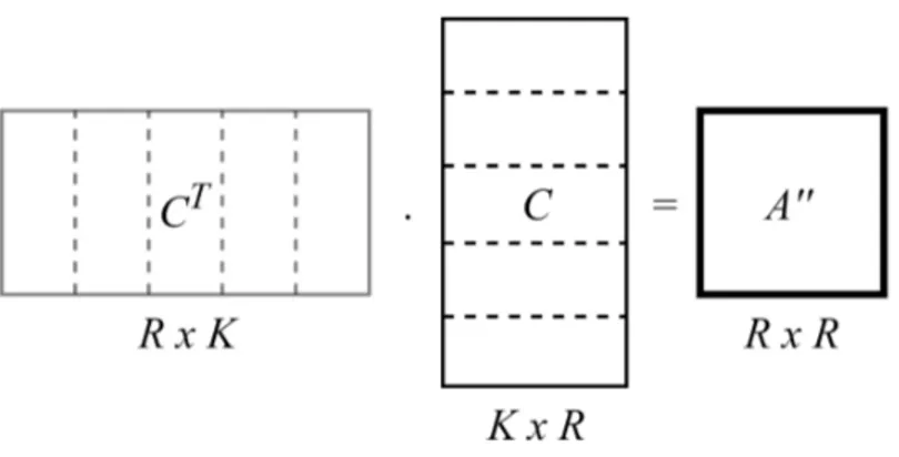
A0 = X(1)(C  B) (2.12)

A00= (CTC ∗ BTB)† (2.13)

2.2.2

MTTKRP

Matricized Tensor Times Khatri-Rao Product (MTTKRP) is defined in (2.12) and is basically the product of two matrices; the first level unfolding of tensor X and the Khatri-Rao product of C and B, where A0 _{∈ R}I×R_{, B ∈ R}J ×R_{, C ∈ R}K×R_,

X(1) _{∈ R}I×J K _{and (C  B) ∈ R}J K×R_.

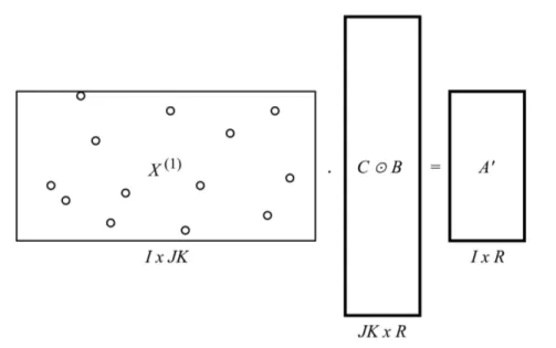
Figure 2.2: MTTKRP Operation, Naive

The inherent problem with this operation is the size of the intermediate matrix (I × J K) being too huge, also known as Intermediate Data Explosion problem. It becomes infeasible to calculate the Khatri-Rao product naively (Figure 2.2). This can be addressed by directly calculating A0 in an indirect element-wise manner, without materializing (C  B) [3]. A0[i, r] = K X k=0 C[k, r] J X j=0 B[j, r]X [i, j, k] (2.15) Example: X = " 0 1 7 0 0 2 3 0 8 6 0 4 9 0 1 2 5 0 #

B =     1 2 2 1 1 3     , C =     3 1 1 1 2 3     C  B =                    3 2 6 1 3 3 1 2 2 1 1 3 2 6 4 3 2 9                    X(1)(C  B) = " 58 115 40 57 #

This calculates A0 according to (2.12). Each element in X is multiplied with B and C then the sum in the last matrix multiplication becomes the result.

A0[0, 0] = 2 X k=0 C[k, 0] 2 X j=0 B[j, 0]X [0, j, k] = 3(1 × 0 + 2 × 1 + 1 × 7) + 1(1 × 3 + 2 × 0 + 1 × 8) + 2(1 × 9 + 2 × 0 + 1 × 1) = 3(9) + 1(11) + 2(10) = 58

This calculates the first cell of A0 according to (2.15), only to find the same result since two formulas are equivalent. The difference is (2.15) is expressed in a series of operations without explicitly materializing the intermediate matrix.

Exploiting the sparsity of the input tensor via bounding to the non-zero count rather than the dimension lengths allows a scalable execution [6].

(3.1) shows an updated version that calculates an entire row of A0 instead of a single cell.

2.3

Apache Spark

Apache Spark is a modern general-purpose parallel programming framework for large scale processing. It was initially developed at Berkeley’s AMPLab and later the codebase was given to Apache Foundation and Apache Foundation continues to maintain and extend its functionalities.

It was developed to address some practical and operational limitations of MapReduce paradigm, which uses a linear flow of computations in which a map task reads data from disk and transforms it, then a reduce task aggregates or applies a collaborative function on it, finally storing on disk again. Spark’s re-markable implicit data parallelism paradigm, also known as Resilient Distributed Dataset (RDD), provides a distributed memory-like approach to this problem by not requiring the materialization of data between intermediate operations by al-lowing the next job to use the data from the distributed memory through building directed acyclic graphs (DAG) that represent computational steps. Together with a rich software ecosystem, this paradigm allows a wide range of applications to be developed, including but not limited to, batch processing, stream processing, data warehousing and monitoring, interactive data analysis, iterative algorithms, parallel algorithms, scientific computations and machine learning.

Spark has built-in fault tolerance that allows automatic recalculations of dis-tributed data partitions due to node failures. This feature is more prominent for clusters made up with commodity hardware on top of commodity networks, and the possibility of a node failure in the cluster increases rapidly as the number of machines increases.

Spark programs consist of a driver program; it invokes parallel operations on RDDs by passing lambda functions to the master node, which then in turn schedules and coordinates executions on worker nodes [7].

2.3.1

RDD Operations

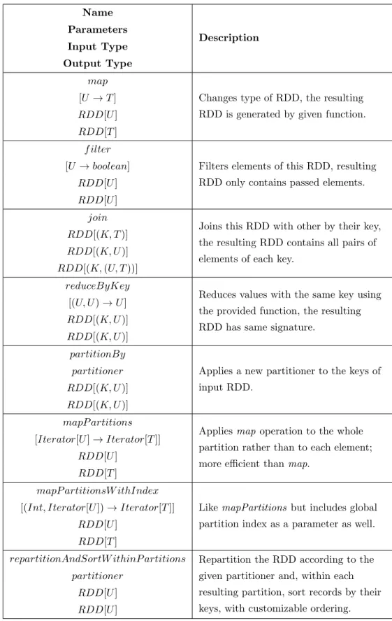
Resilient Distributed Datasets can be imagined as big, distributed, unmaterial-ized and fault-tolerant datasets, partitioned across the entire cluster. An RDD represents an immutable logical data state on which further operations can be applied to produce new RDDs. Operations to be applied on RDDs are two of a kind; transformations and actions. Transformations are functions that produce new RDDs from existing RDDs, e.g., Map is a transformation that produces a new RDD formed by passing each element of input RDD. More types of transfor-mations with their input and output types can be seen in Table 2.1. Actions are functions that mark the end step of an input RDD, by consuming it in the process then either computing some output value or doing other useful work, e.g., Count is an action that counts the number of elements in the input RDD; its output is an integer number. More types of actions with their input and output types can be seen in Table 2.2. All transformations are evaluated lazily, e.g., the com-putation only takes place when an action is applied at the end of given RDD’s lifetime. The Spark scheduler builds a directed acyclic graph (DAG) to plan the transformations to be executed until the action step. These operations are writ-ten as lambda functions by the programmer, then the driver program serializes and distributes them to the worker nodes, which then run them on their portion of RDDs in parallel.

Name Description Parameters Input Type Output Type map

Changes type of RDD, the resulting RDD is generated by given function. [U → T ]

RDD[U ] RDD[T ] f ilter

Filters elements of this RDD, resulting RDD only contains passed elements. [U → boolean]

RDD[U ] RDD[U ]

join

Joins this RDD with other by their key, the resulting RDD contains all pairs of elements of each key.

RDD[(K, T )] RDD[(K, U )] RDD[(K, (U, T ))]

reduceByKey

Reduces values with the same key using the provided function, the resulting RDD has same signature.

[(U, U ) → U ] RDD[(K, U )] RDD[(K, U )] partitionBy

Applies a new partitioner to the keys of input RDD.

partitioner RDD[(K, U )] RDD[(K, U )] mapP artitions

Applies map operation to the whole partition rather than to each element; more efficient than map.

[Iterator[U ] → Iterator[T ]] RDD[U ]

RDD[T ]

mapP artitionsW ithIndex

Like mapPartitions but includes global partition index as a parameter as well. [(Int, Iterator[U ]) → Iterator[T ]]

RDD[U ] RDD[T ]

repartitionAndSortW ithinP artitions Repartition the RDD according to the given partitioner and, within each resulting partition, sort records by their keys, with customizable ordering. partitioner

RDD[U ] RDD[U ]

Each RDD generated via transformations represents an on-the-fly immutable state of a dataset. Once used with next transformation or action, they need to be recalculated again from the start. To reuse RDDs later without the performance penalty of recalculating, they need to be marked as persistent by the programmer. It is possible to store this transient state of data in memory or disk, or to serialize it using a fast serialization library of choice. Caching RDDs in memory across the cluster is a unique feature of Spark, which allows faster execution times via not requiring the intermediate data to be serialized to disk. On the contrary, classic MapReduce needs writing to distributed storage at the end of each computation step. Name Description Parameters Output Type count

Returns the count of elements in this RDD.

− Long collect

Collects all elements of this RDD from the cluster to the driver. −

Iterable[U ]

collect Applies given function to all elements of input RDD (without collecting to the driver).

[U → U nit] −

reduce Reduces all elements of input RDD to one output element using the given function

[U → U ] U

Table 2.2: Action Operations

2.3.2

Partitioning

The partitioning of Pair RDDs (RDDs that consist of key and value tuples) is done with a partitioner function; a function takes an element and outputs a partition number for that element. Each worker holds consecutive partitions of data, e.g., if there are 20 partitions and 4 workers, each worker gets 5 consecutive partitions. Spark applies hash partitioning by default; the hash of the element becomes its partition, which omits data locality. Doing custom partitioning with

respect to data helps improving locality and reducing communication with other workers.

2.3.3

Persistence

Caching in Spark is very important for its performance benefits. Remember that RDD operations (transformations and actions) are applied according to the generated job DAG, based on the operations performed on driver program. Once an operation is applied on an RDD, it consumes the RDD data either to get another RDD (transformation) or a result (action). If the driver program requires the intermediate RDD again, Spark will reapply the operations from the start. If there are some re-used RDDs, this behavior may cause too many recalculations which translate into a poor performance.

Spark’s persistence feature allows to mark RDDs as persistent, which will save the RDDs data to memory or disk, so when that RDD is reused in a later step, it will be served directly from the persisted location, skipping calculations up until the persisted point.

In Hadoop, after every map and reduce operation, the results are written back to HDFS by some Writer. Then, the next job (map and reduce pair) reads that data back from HDFS via some Reader. Since HDFS must be involved between every pair of jobs, it is not performant enough compared to in-memory caching, which Spark takes advantage of.

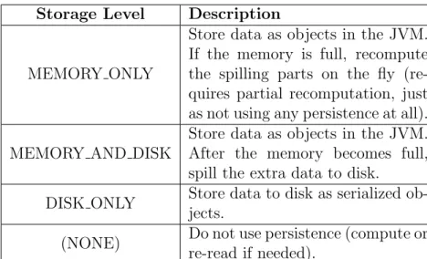
There are multiple storage levels in Spark, which control where and how the data will be stored, shown in Table 2.3. RDDs are not persisted, by default. It is logical because most RDDs are intermediate RDDs between two transformations and they are usually used only once. When desired, an RDD can be persisted by calling persist(storageLevel) on them. This call would mark the RDD as persistent and the framework will persist (or cache) the data of this RDD the first time it is computed and will use the persisted data when the data is requested subsequently. Programmer can unpersist an RDD by calling unpersist().

Storage Level Description

MEMORY ONLY

Store data as objects in the JVM. If the memory is full, recompute the spilling parts on the fly (re-quires partial recomputation, just as not using any persistence at all). MEMORY AND DISK

Store data as objects in the JVM. After the memory becomes full, spill the extra data to disk.

DISK ONLY Store data to disk as serialized ob-jects.

(NONE) Do not use persistence (compute or re-read if needed).

Table 2.3: Storage Levels in Spark

2.3.4

Executor Settings

There are a couple of runtime parameters that Spark accepts in order to optimize the executor and memory allocations, which need to be optimized for each cluster to be as efficient as possible. They control the number of executors, cores per executor and memory per executor, which affect parallelism and throughput of the application. [8] shows there are three main approaches to set these parameters; tiny executor setting essentially creates one executor per core, fat executor setting creates one executor per node and hybrid executor setting which focuses on fixing cores per executor (4 for our application) and generating the runtime parameters around this value. We confirmed that Tiny and Fat executor settings each perform subprime compared to Hybrid setting according to our experiments.

E = (N × (Cn− 1)) ÷ Ce− 1 (2.16)

Me = 0.93 × Mn÷ ((E + 1) ÷ N ) (2.17)

Let N be the total number of nodes in the cluster, Cn be number of cores per

node, Mn be the amount of memory per node, E be the number of executors

executor. N , Cn and Mn are known via the cluster property, Ce is chosen to

be 4, and equations 2.16 and 2.17 calculate E and Me respectively according to

hybrid setting definition of [8], plus a memory adjustment of 0.93 to account for the other processes on every node.

2.4

Prior Art

Kolda and Bader [9] published algorithms to avoid intermediate materialization of the Khatri-Rao product, which led to new implementations on distributed memory and Hadoop systems.

DFacTo [10] is a distributed memory kernel written in C++ Eigen library. It was reported to be significantly faster than GigaTensor and MATLAB CPALS, but was surpassed later on.

Distributed Memory SPLATT (DMS) in [1], [2] and [6] is the most efficient public implementation of PARAFAC-ALS that runs on distributed memory sys-tems with MPI or shared memory syssys-tems with OpenMP.

GigaTensor [3] is an outdated implementation of PARAFAC-ALS on Hadoop. It was released in 2012 and was one of the first papers that explore Tensor De-composition problem on Hadoop. It solved the scalability problem by using a fully distributed system for the MTTKRP step, but this was causing too much communication overhead and not scaling so well.

HaTeN2 [4] is an efficient implementation on Hadoop, which carefully re-orders operations and unifies Tucker and PARAFAC decompositions into a gen-eral framework. They synthetically generate tensors to compare scalability with respect to mode lengths and density.

Parallel PARAFAC [5] is also an Hadoop implementation of PARAFAC which experiment different slicing techniques for long and narrow tensors, instead of tensors with arbitrary shapes. They compare their results with HaTeN2; for the

non-zero experiment, while HaTeN2 turns out to be faster for low nnz numbers, Parallel PARAFAC claims to perform better for high nnz values.

Chapter 3

Methods

The PARAFAC algorithm optimized for Spark will be explained in this chapter. First, we will explain the RDD representations used throughout the implementa-tion. We will then move on to explaining how we implemented specific operations in the PARAFAC algorithm on Spark, including decisions made and optimizations performed. After explaining the details of each operation, we will provide a big picture of all operations working together to complete the PARAFAC algorithm. Later comes the essential optimizations such as Caching, Grid Partitioning, CSR processing, and Multi-Mode Partitioning. The careful and selective application of these optimizations are the vital contributions of this thesis.

3.1

RDD Representations

Let X be a three-dimensional sparse tensor with sizes I × J × K. A real-world tensor is almost always stored in Coordinate Format, i.e., consisting of nnz(X ) rows for each tuple (i, j, k, value). It is usually not preferred to store real-world tensors in either Dense Form or CSR Form for the reasons that they are usually very sparse and CSR requires at least 2 separate arrays (files) to be read, which is not practical for storage purposes. Our program will be reading the tensors in

COO format.

To apply partitioning to RDDs based on their indices, we need to enclose the indices so the RDD typing becomes ((i, j, k), value). This means storing a number of ((i, j, k), value) typed elements distributed across the worker nodes.

Factor matrices of A, B and C have three representation forms; distributed, dense and hybrid. Their dimensions are (I ×R), (J ×R) and (K ×R), respectively. R is a small number (≈ 10), on the other hand, I, J and K typically reach millions. Therefore the factor matrices are usually thin and long matrices.

Distributed Form packs each row of the matrix into one small array with length R and distributes these rows with their indices as an RDD. So the RDD typing of each of these factor matrices becomes (index, row). In other words, each element of this RDD will map to one row from the factor matrix, including the index of the row and the values in the row. The index of the row is needed because the contents of RDDs are unordered. This scheme allows distributing both calculation and storage of factor matrices on the worker nodes. Without RDD representations, the matrices would need to be fit into a single machine’s memory. Distributed Form is suited for matrices that need to be fully distributed because computational work demands so and provides ease of programming at best, but the bookkeeping adds significant additional overhead.

Dense Form, as one can guess, stores the matrix as a full 2D array. When the size of the matrix is small enough, it makes a significant difference vs. using Distributed Form as it is free of bookkeeping overheads. As dimension sizes become larger, using Dense Form increases communication volume unnecessarily, unless the entire matrix will be needed in every executor.

Hybrid Form splits the factor matrix into many small Dense Form matrices on dynamically assigned row intervals. This approach allows executors to only fetch required chunks, instead of requesting rows one-by-one compared to the Distributed Form and the entire matrix in Dense Form.

distribute and operate on huge matrices and the speed of local computation by utilizing cache coherency, assuming the desired computation can be split along the dimension without needing communication between pairs of out-of-order rows.

3.2

MTTKRP

Figure 3.1: MTTKRP Operation, Simplified

A0[i, :] = K X k=0 C[k, :] J X j=0 B[j, :]X [i, j, k] (3.1)

(3.1) is an improved version of (2.15) where cell-wise computation is replaced by row-rise computation. Since R ≈ 10, doing whole row at a time makes it more efficient due to improved data locality and reduced upkeep costs.

Each row of A0 is calculated by multiplying and summing with B and C across the relevant slice in tensor X . In Figure 3.1, we see tensor X , factor matrices B and C, in the middle of calculating ith row of A0, according to (3.1).

Algorithm 2 MTTKRP on Spark, Naive

Require: X is a three-dimensional tensor with size I × J × K. B and C are distributed form factor matrices. A0 is the intermediate matrix for calculating factor matrix A.

1: join (k, i, j, X [i, j, k]) and C[k, :] on k

2: for each X [i, j, k], i, j, k in X do

3: map (i, j, X [i, j, k] · C[k, :]) as Q

4: end for

5: join (j, i, Q[i, j]) and B[j, :] on j

6: for each (i, j, Q[i, j]) in Q do

7: map (i, Q[i, j] · B[j, :]) as Q0

8: end for

9: A0[i, :] ← reduce Q0[i, :] by i then P array Q0_[i]

Algorithm 2 shows the first Spark version of (3.1), which calculates A0 by multiplying nonzeros in X with factor matrices B and C and apply reduction then sum to obtain updated values. Note that this approach uses RDD transformations map, join and reduceByKey to shuffle and gather values on indices therefore X is stored in COO format and B and C are in distributed form. This is a symbolic description of MTTKRP in Spark and will be rewritten to accommodate further improvements in subsequent sections. We aim to make this calculation distributed in Spark but also want to enforce high local computation power with as little communication as possible. Example (i=0, r=0) → " X [0, 0, 0] X [0, 1, 0] X [0, 0, 1] X [0, 1, 1] # → join with C → " X [0, 0, 0]C[0, 0] X [0, 1, 0]C[0, 0] X [0, 0, 1]C[1, 0] X [0, 1, 1]C[1, 0] # → sum columns →hXC[0] XC[1] i → join with B →hXC[0]B[0, 0] XC[1]B[1, 0] i → sum rows →A0[0, 0]

3.3

Caching & Reordering of Computations

Algorithm 3 PARAFAC-SPARK, Naive

Require: X is RDD representation of input the tensor with size I × J × K. A, B and C are RDD representations of factor matrices.

Functions are named after operation names in subsequent sections.

1: for main loop do

2: A ← mttkrp(X , C, B) 3: A ← dstmm(A, hadamardInverse(trmm(C), trmm(B))) 4: A ← normc(A) 5: 6: B ← mttkrp(X , C, A) 7: B ← dstmm(B, hadamardInverse(trmm(C), trmm(A))) 8: B ← normc(B) 9: 10: C ← mttkrp(X , B, A) 11: C ← dstmm(C, hadamardInverse(trmm(B), trmm(A))) 12: C ← normc(C) 13: end for

Algorithm 3 defines the main loop of PARAFAC-SPARK with all operations discussed in subsequent sections. We will apply reordering to reduce redundant operations and caching to take advantage of powerful caching features in Spark. Performance boost of caching (Section 2.3.3) is related to the reuse factor of each RDD after initially materializing it. Zero reuse means zero benefits minus the storage bookkeeping costs; thus we must make sure to apply it on reused RDDs. Input tensor X is the most reused tensor with three reuses per iteration. The construction of a partition of X consists of partially reading a file line by line. If we do not apply any storage level to X , there will be no extra disk or memory usage and no bookkeeping costs, but parsing data cost is higher than reading already parsed data in serialized form. If we apply DISK ONLY level, it will parse the text only once but actual read performance will still be bound to disk, and there will be temporary disk storage costs for the newly allocated files leading to high first iteration and bookkeeping costs. If we apply MEMORY ONLY, the memory will be used for re-reading data with no disk read involved, but it has still some bookkeeping costs and it needs much more memory than the file size

and when there isn’t enough memory the spill would lead to more bookkeeping and less performance.

To apply persistence properly in the main loop, we need to understand the behavior of each operation in terms of RDDs. Every operation type has different semantics; mttkrp applies transformation on three RDDs, trmm applies action on RDD and produces local matrix, dstmm applies transformation on RDD, normc applies one action then one transformation on RDD. Note that transformation and action are Spark terms discussed in Section 2.3.1.

We must avoid recalculation of factor matrices, and such recalculations occur during actions. The best practice is to persist before actions and bring actions closer to each other as much as possible. The latter is already applied with the reordering: normc and trmm operations have both actions and calls to those functions are very close to each other. We should persist after dstmm and before normc calls, one time for each factor matrix. Storage level of these matrices should be MEMORY AND DISK since we must avoid recalculation at all costs. Algorithm 4 shows applied reorderings and persistence calls.

3.4

Dense Form Factor Matrices (DFFM)

Using distributed form with factor matrices requires using Spark’s join transfor-mation to retrieve relevant rows of factor matrices during MTTKRP operation in (2). It results in a global shuffle of data on join key, which needs to be reset before joining with map transformation, adds additional complexity and book-keeping on top of the distributed data. This is not efficient enough for our needs, and we want to eliminate these calls and utilize local computation as much as possible.

Using Dense Form for factor matrices and broadcasting them to all executors would allow us to replace expensive join operations with simple map operations

Algorithm 4 PARAFAC-SPARK, with reordering & caching

Require: X is RDD representation of input the tensor with size I × J × K. A, B and C are RDD representations of factor matrices.

AtA, BtB, CtC are local transpose matrices of respective factor matrices. Functions are named after operation names in subsequent sections.

1: X ← persist(X , MEMORY ONLY) 2: CtC ← trmm(C)

3: BtB ← trmm(B)

4: for main loop do

5: A ← mttkrp(X , C, B)

6: A ← dstmm(A, hadamardInverse(CtC, BtB))

7: A ← persist(A, MEMORY AND DISK)

8: A ← normc(A)

9: AtA ← trmm(A)

10:

11: B ← mttkrp(X , C, A)

12: B ← dstmm(B, hadamardInverse(CtC, AtA))

13: B ← persist(B, MEMORY AND DISK)

14: B ← normc(B)

15: BtB ← trmm(B)

16:

17: C ← mttkrp(X , B, A)

18: C ← dstmm(C, hadamardInverse(BtB, AtA))

19: C ← persist(C, MEMORY AND DISK)

20: C ← normc(C)

21: CtC ← trmm(C)

that make use of the broadcast factor matrices. This change seems to add com-munication overhead to the system, but we have found that it results in great runtime improvements compared to using join transformations which seem to add far too much communication and bookkeeping overhead. We use Spark’s Torrent-Broadcast implementation which can efficiently distribute large data objects in small chunks across the cluster via P2P transfers.

The size of the broadcast grows linearly with the size of factor matrices. Table 4.2 highlights the real world tensors that we will use for evaluation and the size of broadcast for a matrix of size (J × R) is 8J R bytes plus administration overhead. As an example, for J = 105 and R = 10, the size is 8 MiB.

Algorithm 5 MTTKRP on Spark, DFFM

Require: X is a three-dimensional tensor with size I × J × K. Require: B and C are factor matrices in Dense Form.

Require: A0 is the intermediate matrix for calculating factor matrix A.

1: Broadcast B and C

2: for each (i, j, k, X [i, j, k]) in X do

3: emit tuple (i, X [i, j, k] · C[k, :] · B[j, :]) as Q

4: end for

5: A0[i, :] ← reduce Q[i, :] by i then P array Q[i]

The change can be seen in Algorithm 5; instead of join operation, factor matrices B and C are broadcast at the start of the main loop. Therefore, it allows direct access to the factor matrices in the loop, which makes it possible to remove all join calls in each iteration by replacing all transformations with a single map function call. This change effectively applies Dense Form for factor matrices to cut down Spark’s bookkeeping costs. This is useful to understand the impact of using different runtime forms of the same data but still not ideal as larger factor matrices would increase memory and communication costs of the broadcast. In the subsequent section, we will use Hybrid Form for trimming down memory and communication costs.

3.5

Grid Partitioning

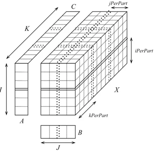
Recall from Section 2.3.2 that Spark RDDs consist of partitions, assigned by a partitioner function, which allows the programmer to adjust the shape and locality of the data. Input tensor X and factor matrices A, B and C as well can be partitioned along their dimensions. When X is imagined as a giant 3D rectangular prism, each partition of X would be a rectangular prism, cut at approximately equal intervals for every dimension; which -together with all partitions- would make up all the cells of X . This results in increased data locality as every partition can now be processed as a whole with less Spark overhead, rather than shuffled and processed randomly among the entire cluster.

Along with X , the factor matrices A, B and C are also partitioned with the same cut points that correspond to the partition cut points of X for every dimen-sion and relevant factor matrix (Figure 3.2). Partitioning a Dense Form factor matrix requires storing the contents of the whole matrix in multiple separate 2D arrays, one for every part of the whole matrix, which in turn effectively form a Hybrid Form factor matrix.

MTTKRP step is then tweaked to only request and access the matching par-tition of every factor matrix, by using a lazy broadcast handle for each part of Hybrid Form factor matrix, which allows a selective broadcast logic to be imple-mented to only retrieve the data precisely needed for current step, as opposed to having access to the whole factor matrix unnecessarily. This reduces active executor memory and the communication volume for the distribution of factor matrices during every iteration. Nevertheless, this change also requires some im-plementation overhead to align indices of local partition to those of global tensor and vice versa at the beginning of MTTKRP core step, which is trivial for larger tensors.

The total number of partitions and number of partitions per dimension are de-noted with N Ptotal, N PI, N PJ, N PK, respectively, where N Ptotal = N PI× N PJ×

Figure 3.2: Grid partitioning

respectively. Global dimension start indices of P with respect to X are denoted with SIP, SJP and SKP, respectively. Position (indices) of partition P alongside

X for each dimension are denoted with P IP, P JP and P KP, respectively, where

P IP ∈ [0..N PI), P JP ∈ [0..N PJ) and P KP ∈ [0..N PK). Number of nonzero

values of P is denoted as nnzP.

During recalculation of each factor matrix in MTTKRP, each partition works toward a relevant part of A0, B0 or C0, together with the other partitions in the same row, during which the intermediate memory usage for partition P becomes O(IP × R), O(JP× R) or O(KP × R), with respect to the factor matrix getting

build.

The total amount of intermediate memory used across all partitions is also an important metric to measure, though it does not accurately reflect the actual

memory used in the cluster as the computation for each partition can be handled independently, without any requirement of allocating that much memory at a given instant. It can be expressed as O(N Ptotal× R × I ÷ N PI), O(N Ptotal× R ×

J ÷N PJ) or O(N Ptotal×R×K ÷N PK); then simplified to O(N PJ×N PK×I ×R),

O(N PI× N PK× J × R) or O(N PI× N PJ× K × R), with respect to the factor

matrix getting built. This definition will be useful in the upcoming sections to show improvements.

We then replace MTTKRP kernel with a single lambda function to be applied locally on each executor for its assigned partitions as a whole, via mapParti-tionsWithIndex transformation, rather than general-purpose transformations like reduceByKey and join. This change requires additional programming for mapping of global indices to local partition indices and vice versa and handling of Hybrid Form factor matrices. With this change, a fine-grained control over the core ker-nel on every executor can be utilized, instead of relying on the general purpose join and aggregation framework of Spark. This lambda function is applied on every grid partition of the input tensor and outputs a partial factor matrix and its partition index. They would then be folded with the partial factor matrices with the same partition index to produce the entire factor matrix to be used in DstMM and NormC operations.

The updated MTTKRP Algorithm 6 operates on the entire partition then outputs the intermediate A0 matrix. It works with factor matrices in Hybrid Form by using lazy global broadcast handles to retrieve only the relevant part of factor matrices selectively. This is made possible by partitioning factor matrices and X at the same cutoff points for every dimension. indices now need to be mapped from global to local according to partitioning specifications, since all factor matrices relevant to each partition are distributed as small 2D matrices but the coordinate format data maintains global indices. We shall name this baseline implementation as PS-COO.

There is a fine balance for finding the best granularity along every mode. A high number of partitions could cause diminishing returns due to increased bookkeeping and context switching costs. On the other hand, less number of

Algorithm 6 MTTKRP on Spark (first dimension shown only), HFFM, PS-COO Require: X is a three-dimensional grid partitioned tensor with size I × J × K,

in COO form.

Require: BHF F M and CHF F M are lazy broadcast handles of factor matrices in

Hybrid Form.

Require: A0 is the intermediate matrix for calculating factor matrix A.

1: for each partition P in X , apply following transformation do

2: SIP, SJP, SKP ← global start indices of P

3: IP, JP, KP ← dimension lengths of P

4: P IP, P JP, P KP ← partition indices of P

5: CP ← retrieve CHF F M[P KP]

6: BP ← retrieve BHF F M[P JP]

7: M AIN ← allocate array[IP][R]

8: for each tuple (i, j, k, X [i, j, k]) in P do

9: i0 ← i − SIP

10: j0 ← j − SJP

11: k0 ← k − SKP

12: increment M AIN [i0][:] by CP[k0][:] · BP[j0][:] · X [i, j, k]

13: end for

14: for idx = 0 to IP do

15: emit tuple (idx + SIP, M AIN [idx]) as Q

16: end for

17: end for

Algorithm 7 Finding optimal partition counts [1] Require: N Ptotal← total partition count target.

Require: DIM ← array of dimension lengths (i.e., [I, J, K])

1: P F ← prime factors of N Ptotal in descending order

2: N P ← allocate array[length(DIM )]

3: N P [i] ← 1 for every i

4: target ← (Plength(DIM )

i=0 DIM [i]) ÷ N Ptotal

5: for pf ← 0 until length(P F ) do

6: f urthest ← 0

7: distances ← allocate array[length(DIM )]

8: for i ← 0 until length(DIM ) do

9: distances[i] ← (DIM [i] ÷ N P [i]) − target

10: if distances[i] > distances[f urthest] then

11: f urthest ← i 12: end if 13: end for 14: N P [f urthest] ← N P [f urthest] × P F [pf ] 15: end for 16: return N P

partitions means reduced parallelism but bigger pieces of data to work on. The granularity of partitions are controlled by the partition count parameters N PI,

N PJ and N PK, one for every mode, respectively. They are input parameters to

the program, however, it is more desirable if those could be assigned automatically in an optimal way regarding the input tensor properties. While determining the partition counts, allocating higher number of partitions along longer modes increases cluster utilization during the fold operation. To automate the selection of partition counts, we adapt the algorithm given in [1] (Algorithm 7). It generates N P , number of partitions per each mode, by first finding prime factors of N Ptotal

then assigning them to each mode starting from the largest prime factor, while selecting largest mode and rotating them via dividing their lengths by the assigned prime factors until there is no more prime factor left. In the end, N Ptotal = N PI·

N PJ · N PK holds true and every mode gets assigned a fair number of partitions

depending on their length. It was observed that this automatic assignment scheme always results in a better or similar level of performance than manual assignment of partition counts.

3.6

Compressed Sparse Row (CSR) Processing

Compressed Sparse Row (CSR) format for the input tensor explained in Sec-tion 2.1.3.3 is the tensor processing format in MTTKRP kernel of Distributed Memory SPLATT [6] due to its cache locality and reduced memory overhead. We aimed to utilize CSR format in our Spark MTTKRP kernel for faster execu-tion, by utilizing grid partitioning method from PS-COO and creating separate CSR structures for each partition P in X then modifying MTTKRP to work on these separate CSR structures locally within each partition. Since input ten-sors are supplied in COO format, they need to be partitioned first, then a CSR structure for each partition is created, according to the same partitioning spec-ifications. For each partition P of a 3D input tensor X , this means a single big tuple that holds four one dimensional arrays for the three dimensions and one for the non-zeros in CSR. This implementation will continue to utilize Hybrid Form for factor matrices and partition alignment features of PS-COO thus taking ad-vantage of selective distribution of factor matrices with efficient communication. We shall call this implementation as PS-CSR.

The choice of major dimension in CSR format determines the processing direc-tion of the input tensor, and a single CSR form would not suffice to run MTTKRP step without a huge intermediate memory. According to [1], only two CSR forms are enough to process the tensor to efficiently calculate factor matrices, instead of one form for every mode. Therefore, we prepare two CSR forms of the input tensor by implementing an additional preprocessing stage (Algorithm 8). The two smallest modes will be marked as major dimension of the CSR index array to save maximum space. For example, if the smallest modes are first and third, we prepare two cached CSR forms: one form with first mode as major and one form with third mode as major. The ordering of non-zeros is also important in the processing order. Algorithm 8 shows the preprocessing of a CSR form with first mode as major. The resulting CSR forms are cached in memory or disk using Spark’s caching feature, so this process is only applied once per decomposition. Tables 3.1 and 3.2 show the two CSR forms, their sort modes and the which mode is used while calculating the factor matrices.

Algorithm 8 Preprocessing a 3D tensor to generate a CSR Form for every partition

Require: X is a three-dimensional grid partitioned tensor with size I × J × K.

1: for each partition P in X do

2: SIP, SJP, SKP ← global start indices of P

3: IP, JP, KP ← dimension lengths of P 4: P IP, P JP, P KP ← partition indices of P 5: nnzP ← number of nonzeros in P 6: CIP ← allocate array[IP] 7: CJP ← allocate array[nnzP] 8: CKP ← allocate array[nnzP] 9: CVP ← allocate array[nnzP] 10: CI[0] ← 0 11: lastI ← 0 12: index ← 0

13: Sort in-place tuples (i, j, k, X [i, j, k]) in P by i then j ascending

14: for each tuple (i, j, k, X [i, j, k]) in P do

15: i0 ← i − SIP 16: CJP[index] ← j − SJP 17: CKP[index] ← k − SKP 18: CVP[index] ← X [i, j, k] 19: if lastI 6= i0 then 20: while lastI < i0 do 21: if lastI > 0 then 22: CIP[lastI] ← CIP[lastI − 1] 23: end if 24: lastI ← lastI + 1 25: end while 26: CIP[lastI] ← index 27: end if 28: index ← index + 1 29: end for

30: return and cache (CIP, CJP, CKP, CVP)

Algorithm 9 MTTKRP on Spark (first dimension shown only), PS-CSR

Require: X is a three-dimensional grid partitioned tensor with size I × J × K, in CSR form, major dimension is first. BHF F M and CHF F M are global handles for

partitioned factor matrices B and C.

Require: CSR structure (a tuple of 4 arrays) of every partition of X is sorted internally by i then j.

1: for each partition P in X do

2: (CIP, CJP, CKP, CVP) ← CSR structure of P 3: SIP, SJP, SKP ← global start indices of P 4: IP, JP, KP ← dimension lengths of P 5: P IP, P JP, P KP ← partition indices of P 6: nnzP ← number of nonzeros in P

7: BP ← retrieve BHF F M[P JP] 8: CP ← retrieve CHF F M[P KP] 9: M AIN ← allocate array[IP][R] 10: CARRY ← allocate array[R] 11: for i = 0 to IP do

12: start ← CIP[i]

13: end ← if (i == IP− 1) then nnzP else CIP[i + 1] 14: while start < end do

15: j ← CJP[start] 16: k ← CKP[start] 17: if j has changed then

18: increment M AIN [i][:] by CARRY [:] · BP[jprevious][:] 19: clear CARRY

20: end if

21: increment CARRY [:] by CVP[start] · CP[k][:] 22: start ← start + 1

23: end while

24: increment M AIN [i][:] by CARRY [:] · BP[jprevious][:] 25: clear CARRY

26: end for

27: for each index in M AIN do

28: emit tuple (index + SIP, M AIN [index]) 29: end for

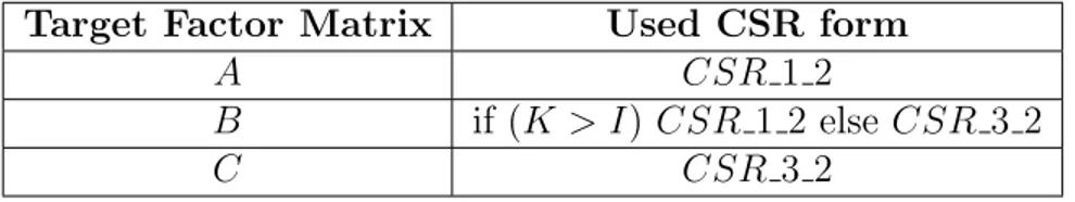
CSR Form Sort By

CSR 1 2 (i, j)

CSR 3 2 (k, j)

Table 3.1: CSR Forms

Target Factor Matrix Used CSR form

A CSR 1 2

B if (K > I) CSR 1 2 else CSR 3 2

C CSR 3 2

Table 3.2: CSR Form Selection of Factor Matrices

Algorithm 9 shows the core kernel of PS-CSR, whose main structure is similar to Algorithm 6 of PS-COO. The difference is the kernel operates on the 4 one di-mensional arrays of CSR form, resulting in cache locality compared to processing tuples in COO form, with improved runtime, which seems to be correlated with the size of input tensor.

3.7

Multi-Mode Partitioning

During the calculation of A0, B0 and C0for an input tensor X with dimension sizes I × J × K and partition counts N PI, N PJ and N PK, where each partition in the

grid outputs a portion of the resulting factor matrix. Then, the portions with the same offset are folded via addition operation. The size of this intermediate matrix portions are I/N PI, J/N PJ and K/N PK respectively. During the reduction of

each factor matrix, number of reduce jobs are equal to the partition counts of the respective factor matrix, which becomes the limiting factor to the cluster utilization as not all executors can be utilized since E  max(N PI, N PJ, N PK),

where E is the number of executors.

To alleviate this problem, we use different partitioning schemes for factoriza-tion of each factor matrix, which increases the number of reducers to match N P and increase utilization among the cluster. We multiply the number of partitions for the major dimension by a new mmp parameter and divide the number of partitions for the other dimension by the same parameter, for each of the two major dimensions. This change does not change the total number of partitions but changes the shapes of them to favor the first two major dimensions during MTTKRP. We shall call this implementation as PS-CSRSX, where X = mmp.

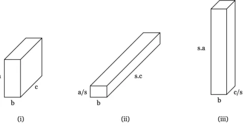
Figure 3.3: Multi-Mode Partitioning (Partition Stretching)

In Figure 3.3, (i) shows a single base partition in the grid, where a, b, c are the lengths of this partition, (ii) shows the resulting partition after applying

MMP to first mode by s and (iii) shows the resulting partition after applying MMP to third mode by s. For example, let mmp = 4, and let partition counts before applying MMP N PI = 16, N PJ = 2, N PK = 32 for all CSR modes. After

applying MMP, partition counts become N PI = 64, N PJ = 2, N PK = 8 for A

and N PI = 4, N PJ = 2, N PK = 128 for C, respectively.

Multi-Mode Partitioning also decreases both the intermediate memory usage of each partition and the total amount of intermediate memory used across all partitions as well, by mmp parameter during MTTKRP step for first and third mode (i.e., according to the scheme in Figure 3.3). This reduction is achieved by the fact that; while the total partition count N Ptotal remains the same, the

amount of intermediate memory used for first and third modes are reduced by mmp, while the memory usage of second mode (the mode for which there is no major CSR form) remains unaffected because the calculation works off a CSR form which is not major relative to the current mode.

Let superscripts mmpi and mmpk denote MMP version of the corresponding

variable during calculation of the first and third mode factor matrices, respec-tively; e.g, let Pmmpi _{denote the resulting partition after applying MMP by mmp}

to P in first mode. The memory usages after applying MMP are found as fol-lows; for first mode partition Pmmpi_{, it becomes O(I}mmpi

P × R), where I mmpi

P =

IP ÷ mmp; for third mode partition Pmmpk, it becomes O(KPmmpk × R), where

Kmmpk

P = KP÷ mmp, an effective reduction by mmp in both modes. Memory

us-age for second mode remains the same as the increase and decrease in number of partitions along first and third order cancel each other out. Furthermore, the to-tal amount of intermediate memory used across all partitions after applying MMP are found as follows; for first mode it becomes O(N Ptotal×R×I ÷N P_Immpi) where

N Pmmpi

I = N PI× mmp, simplified to O(N PJ× N PK× I × R ÷ mmp); for third

mode it becomes O(N Ptotal× R × K ÷ N PKmmpk) where N P mmpk

K = N PK× mmp,

simplified to O(N PJ× N PI× K × R ÷ mmp), an effective reduction by mmp at

the total memory usage level in both modes as well.

Multi-Mode Partitioning narrows the surface of the major form partitions to increase parallelism by utilizing more cores with the reduction, without changing