A Framework for incorporating environmental indicators in the measurement of human well-being

10

A Framework for Incorporating

Environmental Indicators in the

Measurement of Human

Well-Being

Osman Zaim

Introduction

The last decade has witnessed major improvements in the measurement of sustainable human development. Considerable time and research effort have been devoted to both extending the dimensions of the measurement and the methodology used to compute sustainable human development indices. Now, the measurement of human well-being is not only limited to economic indicators but also takes into account social, institutional and ecological background, thus utilizing over 130 indicators approved by the United Nations in April 1995 (UN 2001). Improvements in the data collection of indicators, while triggering the construction of indexes from a series of constituent indicators such as human development index (HDI) with com-ponent indicators on longevity, educational attainment and income, have also led to aggregation of indexes of different dimensions. As a typical example of the latter, one can cite Prescott-Allen's (2001) human well-being index (HWI), which is an equal weighted average of the human well-being index and ecosystem well-being index (EWI), integrating two indices with social-economical and environmental dimensions.

On the academic front, research during recent years has considerably improved our understanding of sustainable human development, but at the expense of generating a certain amount of controversy. The concerns range from not being able to construct a totally objective index of sustain-able human development (because both the indicator selection and weights assigned to these reflect normative judgements of those who developed the index), to whether these indices satisfy the certain axiomatic properties required of any index (Sen 1976; Zheng 1993). Specifically, a consensus has emerged that existing indexes, such as the HDI, fail to measure per-formance comparisons across time, because these are designed to measure performance comparisons at a point of time rather than being a measure of over-time comparisons.1

194 M. McGillivray (ed.), Road Movies

Osman Zaim 195 The purpose of this chapter is to expand on earlier works by Zaim et al. (2001) and Grosskopf et al. (2002) to provide a framework for incorporat-ing environmental indicators to the measurement of human well-beincorporat-ing. Although some prior studies such as Nath et al. (1998), Lasso de la Vega and Urrutia (2001) and Prescott-Allen (2001) all had the same objective of recon-ciling human well-being with environmental indicators, this study with its economic-theoretical approach to index number theory is a deviation. This chapter proposes a useful alternative to the 'aggregate deprivation index' used to measure the well-being of individuals in different countries or geo-graphic locations. Furthermore, an improvement index which alleviates the well-known difficulties associated with over-time comparisons of the aggre-gate deprivation index is also proposed. The achievement index in this study relies heavily on the theory of quantity indexes whose axiomatic properties are well established. The roots of the improvement index are well grounded in the productivity growth literature. All proposed measures depend on the computation of distance functions, which are a complete characterization of technology. The indexes introduced in this study are an improvement of the empirical literature on social indicators in several respects.

First, unlike previous studies which typically produce a synthetic indica-tor that aggregates its constituents using artificially assigned weights, the proposed approach implicitly recognizes the underlying production process which transforms inputs (per capita capital) into private goods (which can be proxied by per capita income), social goods (which can be proxied by longevity and knowledge) and undesired goods (such as emissions of environ-mentally hazardous elements) by putting sufficient emphasis on production with negative externalities. Thus, while providing an economic content to social indicators, the aggregator characteristics of distance functions (which aggregate components with optimally chosen weights determined by the data) are fully exploited. Second, the proposed improvement index, since it is measured with respect to a production technology which is allowed to change over time, can capture the improvement in performance better than alternative indexes which have less tolerance for best achievers.

The next section presents the methodology for constructing a human development index that takes into account differences in the environmental conditions. This is followed by an empirical application and the conclusions drawn.

Methodology

This section follows closely Zaim et al. (2001) and Grosskopf et al. (2002) in order to summarize the methodology for constructing a human develop-ment index void of any environdevelop-mental considerations, so as to prepare the

background for an extension that would allow for the incorporation of envi-ronmental indicators. Let us consider a sample of K countries, each of which produces a vector of private goods denoted by y = (Yl, ... , YM) E R~ and a

vector of social goods s = (sl, ... , SJ) E R~, using inputs x = (XI, ... , XN) E

Rlf_

with a meta technology represented by output (or production possibilities) set as

P(x) = { (y, s) : x can produce (y, s)}

which satisfy certain axioms laid out by Shephard (1970). P.l P(0)={0,0}.

P.2 P(x) is compact for each x E

Rlf_.

P.3 P(x) 2 P(x'), x :::_ x'.

P.4 (y, s) E P(x) andy' ~ y and s' ~ s imply (y', s') E P(x).

(10.1)

Properties P.1 state that zero inputs yield zero outputs and that any non-negative input yields at least zero output. Properties P.2 require that only finite output should be produced given finite inputs. Finally, properties P.3 and P.4 impose free disposability of inputs and outputs, respectively.

Since the ultimate goal is to construct a quantity index for private and social goods that would allow multilateral comparisons across countries, Shephard's output distance functions are a useful tool for both representing technol-ogy and also serving as a measure of performance. Hence, given an arbitrary vector of inputs x0 , once the success of countries i and j in expanding their pri-vate and social goods with respect to a set of production possibilities (output) common to all countries is measured by means of distance functions,

D~(xO,yi) = inf{l:li: x0 , (yi,si)/l:li E P(x)) and

dacx0,yi) = inf(ei: xo, (yi,si);ei E P(x)J (10.2)

this allows for the construction of Malmquist quantity index of (aggregated) social and private goods as

i 0 i i

Q( _{x ,y,y,s,s}

o

i j i j)D

= .

_ _,_o (-'---x_,'-'-Y---''-s_)

d

0(xO, yi, si)

(10.3) This quantity index now compares the provision of social and private goods in country i with respect to a reference country j given an arbitrary vector of inputs x0 _{common to both. Since the meta technology that serves as a} basis for the computation of distance functions is unobserved, it has to be constructed from the observed inputs and outputs of the countries in our sample. For this purpose, an activity analysis or data envelopment analysis (DEA) approach, which satisfies the properties underlying the technology

Osman Zaim 197 (see Fare et al. 1994), is employed. The piecewise linear output set is

K P(x)={(y,s): LZkYkm::':Ym1 m=1, ... ,M k=l K LZkSkj::':Sj, j=1, ... ,J k=l K

L

zkxkn :::: Xn, n = 1, ... , N k=l k=1, ... ,K} (10.4)

where zk are the intensity variables which serve to form the technology from convex combinations of the data.

This quantity index, which is essentially a Malmquist quantity index (see Fare and Primont 1995), satisfies a number of desirable properties due to Fisher (1922). These are

Q(xo,

;,.yi,

yi, A.si, si) = A.Q(xo, yi, yi, si, si)

Qs(XQ I yi I yi I Si, si)Qs(XQ I yi, yi, si I Sj) = 1

(1) Homogeneity: (2) Time-reversal: (3) Transitivity: (4) Dimensionality:

Qs(xo, yi, yi, 5i, si)Qs(xo, yi,

yt,

si, 5t) = Qs(xo, yi,

yt,

5i, 5t) Qs (X0 1 ).yi 1 ).yi 1 A5j 1 A.si) = Qs(x0 1 yi 1 yi 1 Sj 1 si)

As for the improvement index, we measure the success of a particular coun-try in expanding its social goods from year t to year t

+

1 with respect to a common (world) benchmark technology constructed for the period t. Our improvement index

Dk,t(xk,t yk,t+l 5k,t+l)

IMPt,t+l = 0 I I

D~,t (xk,t' yk,t' sk,t) is the ratio of two distance functions where

D~,t (xk,t,yk,t+l, 5k,t+l)

= inf{ek,t+l : (xk,t I cl,t+l, sk,t+l )jek,t+l) E pt (Xt)}

and

(10.5)

(10.6)

The first-distance function shows the success of an observation, say k, in expanding its private and social goods in year t

+

1 (with respect to a common frontier which represents the technology at t) while using the same level as in year t (that is, xk,t). Similarly, the second-distance function measures the success of the same observation in expanding its private and social goods in period t with respect to a common frontier representing the technology

at t. Note that, since the distances are measured against the same benchmark (while holding resources and private goods at their year t levels), the ratio indicates the improvement in the provision of private and social goods for observation k.

To incorporate the joint production of bad outputs b

=

(b1, ... , hi) E R~

(that is, emissions of environmentally hazardous elements, which would ulti-mately affect human well-being negatively), this requires modifications both in our definition of performance measure and also in axiomatic properties of the meta technology. Note that while the Shephard output distance function allows one to construct a human well-being index by aggregating the social and private goods without any normative judgements, it still fails to account for the joint production of goods and bads. The generalization of this index to include bad outputs would not be meaningful (by redefining the output distance function as D0(x,y,s,b) = inf{e: x, (y,s,b)/8 E P(x)}) since it would

mean proportionate expansion of bads together with private and social goods as much as feasible without crediting the reduction of bads. Nevertheless, the directional distance function proposed by Chung et al. (1997), which suggests asymmetric treatment of good and bad outputs, provides a solution by crediting the expansion of good outputs and the contraction of bad out-puts. Letting g = (gy,g5 , -gb) be a direction vector, the directional distance

function is expressed as

Do(x,y,s,b;gy,gs,-gb) = sup[,B: (y

+

,Bgy,s

+

,Bgs,b- ,Bgb) E P(x)]

(10.7) A nice feature of this directional distance function is that, as shown by Chung

et al. (1997), it embodies Shephard's output distance function as a special case.

Letting g = (y, s, b) and following Chung et al. (1997):

D

0(x, y, s, b; y, s, b)= sup{,B : D0(x, (y, s, b)+ ,B(y, s, b) ::: 1}

= sup{/3: (1

+

}3)D0(x,y,s,b)::: 1} { 1 } = sup }3 : }3 < - 1 - D0(x, y, s, b) 1

=

_{Do(X, y, s,} -1 b) or equivalently D0(x, y, s, b) = 1/(1

+

D

0(x, y, s, b; y, s, b) (10.8)

Then, letting g = (y, s, -b), the bads-incorporating human well-being index

can be expressed as

;=,i 0 . . . . Q

o

i ; i ; bi

hi _

1 +u0(x ,yl,sl,bl;yl,sl,-bl)

(X I y 1 y 1 S 1 S I 1 ) - ~ • 0 . , . . , .

Osman Zaim 199 This quantity index now shows the success of country i in equiproportion-ate expansion and contraction of good (social and privequiproportion-ate) and bad outputs respectively, relative to a reference country j. Similarly the bads-incorporating improvement index can be written as

1

+

fl·t (xk,t yk,t 0 I I 5k,t bk,t. yk,t I I I 5k,t -bk,t) I

IMPt,t+l =

----;---.,----,----'---'---,--1 +Dk,t (xk,t yk,t+l 0 I I 5k,t+l bk,t+l-yk,t+l I I I 5k,t+l -bk,t+l) I (10.10)

Now we turn our attention to the axiomatic properties of the output set when some outputs are undesired or associated with negative externalities. In the production theory, it is common to assume that outputs are strongly disposable, which implies that the disposal of any output can be achieved without incurring any costs in terms of reduced production of other outputs. This is, in fact, the case for desired outputs, private and social goods in P.4. However, the symmetric treatment of outputs in terms of their disposability characteristics loses its justification if one or some of the outputs, along with the desired outputs, are undesired goods such as carbon dioxide production (as a by-product). Especially in regulated environments, where the produc-tive unit is forced to clean up its undesired output or to reduce its levels of undesired output production, undesired and desired outputs have to be treated asymmetrically in terms of their disposability characteristics. Even in the absence of regulations, increased environmental consciousness in society still requires the treatment of undesired goods as weakly disposable; that is, their disposal is achieved by reducing the desired outputs proportionately. The following property

P.S (y, s, b) E P(x) and 0 :s () :s 1 imply (ey, es, ()b) E P(x)

imposes weak disposability of good and bad outputs.2 _{It states that for a} given input vector, only a proportional contraction of good and bad outputs is feasible. Finally, one should also recognize the joint product nature of bad outputs. The following property, P.6, is referred to as null-jointness:3

P.6 (y, b) E P(x) and b

=

0 then y

=

0

This implies that for a given output vector, if bad output is zero, then so too must be good output. In other words, if one wishes to produce good output, some bad output will also be produced.

The piecewise linear output set associated with properties P.1-P.6 is (see Fiire et al. 1994): K P(x)={(y,s,b): LZkYkm~Ym, m=1, ... ,M k=l K L ZkSkj ~ Sj, j

=

1, ... ,! k=l K L zkbki

=

bi, i

=

1, ... ,I k=l K L ZkXkn :S Xn, n = 1, ... , N k=l k= 1, ... ,K) (10.11)

where the zk are intensity variables that serve to form the technology from convex combinations of the data. The technology represented in (10.11) also

satisfies constant returns to scale; that is

P(A.x) = A.P(x), A. > 0 (10.12)

The first two inequalities in (10.11) imply that private and social goods are

freely disposable. Since the intensity variables zk, k = 1, ... , K, are non-negative and the bad output constraint is a strict equality, one can show that (10.12) satisfies weak disposability.

Null-jointness requires that

K (i) L bki > 0, i = 1, ... I I k=l I (ii) L bki > 0, i = 1, ... I K i=l

The first inequality requires that each bad output is produced by some firm k, while the second inequality states that each firm k produces some bad output.

Having formed the output set for each of the countries in our dataset k' =

1, ... K, the solution to the following linear programming problem computes

the directional distance:

~ Ok'k'k' D0(x ,y ,s ,b ;g) =maxj3 such that K k k' k' L ZkYm ~ Ym

+

tlYm m = 1, · · ·, M k=l K k k' k'

L

zks. > s.

+

j3s. j

=

1, ... ,J k=l l - l l (10.13) K k k' k' L zkbi = bi - j3bi i = 1, ... ,I k=l K k L zkxn :S xg n = 1, ... , N k=l

Osman Zaim 201 which is in the denominator of (10.9). The directional distance of the ref-erence country in the numerator is computed by replacing the right-hand sides of the first three constraints above with the associated quantities of the country chosen as the reference country, that is, country j.

As for the computation of the improvement index, for each k' the following linear programming problem:

jjk't (xk',l',t+1, bk",t+ 1, yk't+1) =max ek',t+ 1

such that

~

z 5t _ ek',t+1l',t+1 > l+1 L., k kj k'j - k'j k=1

~

z Yt _ ek',t+1yt+1 > yt+1 L k km k'm - k'm k=1

~

z bt

+

ek',t+1bt+1 _ bt+1 kL., k ki k'i - k'i =1 K t t

L

zkxkn _::: xk'n k=1 zk ~ 0 j = 1, ... . ,J m=1, .... ,M (10.14) i = 1, ... . ,I n= 1, .... ,N k = 1, ... ,K

solves for the directional distance function in the denominator of IMPt,t+1.

The numerator can be computed in a similar fashion as

j = 1, ... . ,J m=1, .... ,M _(10.15) i

=

1, ... . ,I n= 1, .... ,N k= 1, ... ,K A numerical example

In constructing the numerical exercise for the human well-being and improvement indexes proposed in this study, data for 22 high income OECD countries are selected for the years 1977, 1980, 1982, 1987, 1990. The reason for restricting the sample to high income countries is twofold. First, since a meta technology that is common to all countries exists, it is desirable that the weak disposability of undesired outputs assumption holds for each country. Otherwise, there is always a danger of over-crediting the comparatively lower emissions of lower income countries who are treating undesired outputs as strongly disposable. In such instances, it may be better to relax the weak

disposability assumption in favour of strongly disposable outputs, but still crediting expansion of desired outputs and contraction of undesired. Second, this allows the demonstration of a couple of stylized facts on the informa-tional validity of HDI. Various studies, specifically Ivanova et al. (1999), in

their assessment of the measurement properties of HDI, find very high corre-lations between the HDI index and per capita GDP of countries. Furthermore, they show that this high correlation is independent of the weights assigned to constituent indices. Therefore, one would expect this to be amplified within a group of high income countries, resulting in an HDI, which is indistinguish-able from per capita income, since all other constituent indices except income are very close to each other. If this is, in fact, the case, it will provide further justification to search for alternative constituent indices or aggregation of indexes of different dimensions.

We proxy the vector of social goods with infant survival rate, life expectancy at birth (total years), primary school enrolment rate (per cent gross) and secondary school enrolment rate (per cent gross). The environ-mental indicator is chosen as per capita carbon dioxide emission. Our proxy for private goods is real gross domestic product per labour. The resource con-straint is represented with an aggregate input, capital stock per labour. The source for the variables representing social goods, and the environmental indicator is the World Bank Social Indicators Database. Other variables, real gross domestic product, capital stock and employment are retrieved from the Penn World Tables which limits extending our data to 1990 only, since revised capital stock estimates are not yet available for later years.

In this particular application, a hypothetical'average country' (in all vari-ables for every year) is chosen as a reference country. Thus, it is assumed that j = 0, which then refers to the associated quantities for the 'average country'.

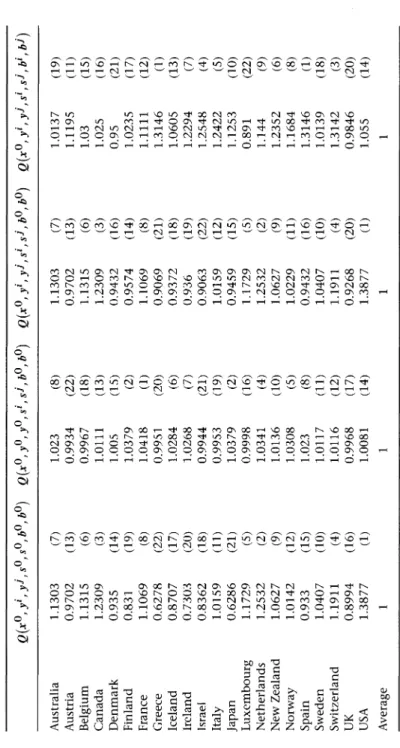
To provide a means of comparison among indexes with different compo-nent indices, a step-by-step approach is followed for the year 1977. First, by holding all variables other than income constant at 'average country' levels, an income index is generated for the year 1977. This index (with associ-ated ranks) is shown in column 1 of Table 10.2. Note that income is almost equally dispersed around the average country with the highest income (USA) and the lowest income (Greece) being approximately 38 per cent above and below average, respectively. Then, the same exercise is repeated for the vector of social goods only, holding income, undesired output and resources at the average country levels. A close examination of column 2 reveals that, with respect to the provision of social goods, high income countries are very sim-ilar to each other, the difference between the best and the worst provision being only 5 per cent. Column 3 is reserved for the traditional HDI, a compos-ite index of social goods and income, but with the weights being determined optimally by the data. The comparison of columns 1 and 3 confirms our prior expectation that, with similar provision of social goods, HDI becomes almost identical to per capita labour income and provides justification for Ivanova, Arcelus and Srinivasan's assessment of the measurement properties

Table 10.1 Alternative indexes of human well-being in OECD countries Q(xO,yi,yi,sO,sO,bO,bO) Q(xo, yo, yo, si, si, bo, bo) Q(xo, yi, yi, si, si, bo, bo) Q(xo, yi, yi, si ,si, bi, bi) Australia 1.1303 (7) 1.023 (8) 1.1303 (7) 1.0137 (19) Austria 0.9702 (13) 0.9934 (22) 0.9702 (13) 1.119S (11) Belgium 1.131S (6) 0.9967 (18) 1.131S (6) 1.03 (1S) Canada 1.2309 (3) 1.0111 (13) 1.2309 (3) 1.02S (16) Denmark 0.93S (14) l.OOS (1S) 0.9432 (16) 0.9S (21) Finland 0.831 (19) 1.0379 (2) 0.9S74 (14) 1.023S (17) France 1.1069 (8) 1.0418 (1) 1.1069 (8) 1.1111 (12) Greece 0.6278 (22) 0.99S1 (20) 0.9069 (21) 1.3146 (1) Iceland 0.8707 (17) 1.0284 (6) 0.9372 (18) 1.060S (13) Ireland 0.7303 (20) 1.0268 (7) 0.936 (19) 1.2294 (7) Israel 0.8362 (18) 0.9944 (21) 0.9063 (22) 1.2S48 (4) Italy 1.01S9 (11) 0.99S3 (19) 1.01S9 (12) 1.2422 (S) Japan 0.6286 (21) 1.0379 (2) 0.94S9 (lS) 1.12S3 (10) Luxembourg 1.1729 (S) 0.9998 (16) 1.1729 (S) 0.891 (22) Netherlands 1.2S32 (2) 1.0341 (4) 1.2S32 (2) 1.144 (9) New Zealand 1.0627 (9) 1.0136 (10) 1.0627 (9) 1.23S2 (6) Norway 1.0142 (12) 1.0308 (S) 1.0229 (11) 1.1684 (8) Spain 0.933 (1S) 1.023 (8) 0.9432 (16) 1.3146 (1) Sweden 1.0407 (10) 1.0117 (11) 1.0407 (10) 1.0139 (18) Switzerland 1.1911 (4) 1.0116 (12) 1.1911 (4) 1.3142 (3) UK 0.8994 (16) 0.9968 (17) 0.9268 (20) 0.9846 (20) USA 1.3877 (1) 1.0081 (14) 1.3877 (1) LOSS (14) Average 1 1 1 1 N 0 w

Table 10.2 Quantity indexes 1977 1980 1982 1987 1990 IMP 1977-90 Australia 77.11 (19) 78.45 (16) 74.28 (18) 75.40 (18) 77.75 (22) 1.01 Austria 85.16 (11) 92.29 (7) 89.83 (11) 84.20 (11) 87.12 (10) 1.12 Belgium 78.35 (15) 80.62 (14) 81.22 (15) 81.60 (13) 88.21 (8) 1.19 Canada 77.97 (16) 76.09 (19) 74.23 (19) 79.20 (14) 85.51 (12) 1.13 Denmark 72.27 (21) 79.19 (15) 78.30 (16) 72.74 (20) 79.63 (20) 1.14 Finland 77.86 (17) 77.98 (17) 82.97 (14) 73.96 (19) 82.73 (16) 1.10 France 84.52 (12) 87.33 (9) 92.72 (8) 94.71 (2) 100.00 (1) 1.25 Greece 100.00 (1) 99.53 (3) 99.06 (4) 86.98 (6) 88.45 (7) 0.92 Iceland 80.67 (13) 84.16 (13) 91.12 (9) 85.16 (10) 84.96 (13) Infeasible Ireland 93.52 (7) 87.32 (10) 87.49 (12) 77.33 (15) 82.00 (18) 1.01 Israel 95.45 (4) 98.95 (4) 94.92 (6) 85.81 (9) 86.59 (11) 0.95 Italy 94.49 (5) 100.00 (1) 99.18 (3) 94.44 (3) 95.12 (3) 1.12 Japan 85.60 (10) 86.33 (11) 86.42 (13) 82.29 (12) 82.30 (17) 0.99 Luxembourg 67.78 (22) 66.79 (22) 67.39 (21) 71.00 (21) 84.26 (14) 1.24 Netherlands 87.02 (9) 87.41 (8) 94.50 (7) 86.17 (8) 88.07 (9) 1.11 New Zealand 93.96 (6) 95.93 (6) 100.00 (1) 86.27 (7) 89.64 (6) 1.01 Norway 88.88 (8) 67.60 (21) 65.84 (22) 67.44 (22) 81.04 (19) 0.89 Spain 100.00 (1) 100.00 (1) 100.00 (1) 100.00 (1) 100.00 (1) 1.28 Sweden 77.13 (18) 85.89 (12) 90.64 (10) 90.16 (5) 92.38 (5) 1.28 Switzerland 99.97 (3) 98.70 (5) 95.61 (5) 91.04 (4) 94.43 (4) 0.99 UK 74.90 (20) 75.73 (20) 77.16 (17) 75.74 (16) 78.24 (21) Infeasible USA 80.25 (14) 76.39 (18) 74.00 (20) 75.67 (17) 83.64 (15) 1.14 Geometric mean 84.62 84.97 85.55 82.19 86.70 1.09

Osman Zaim 205 of the HDI. Note that while the HDI index value for half of the countries is the same as GDP per labour, considerable differences still exist between the two indexes for Finland, Greece, Ireland, Iceland and Japan. Armed with suf-ficient justification for an alternative index, in the last column in Table 10.1, the quantity index in (10. 9)-which shows the success of country i in

equipro-portionate expansion and contraction of good (social and private) and bad outputs relative to a reference country j-is listed. Note that while this index rewards relatively low polluters such as Greece, Spain, Italy, New Zealand and Ireland, it severely punishes high polluters such as Luxembourg, USA, Sweden, Denmark and Canada.

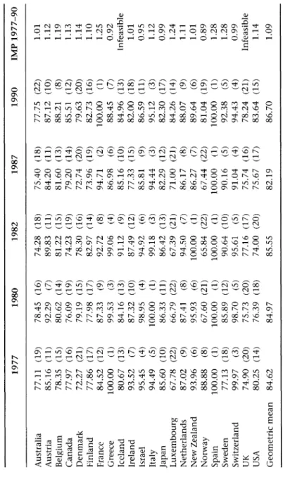
Since this index is transitive, it allows for bilateral comparisons among all country pairs. To facilitate an easier exposition, the bads-incorporating quantity index (10.9) is normalized for each year by the value of the best performer, so as to assign a value of 100 for the best achiever. These are given in Table 10.2, where although the ranking of individual countries dif-fers from year to year, Switzerland, Spain, and Italy have always maintained their position within the best five performers. As for the worst performers, our bads-incorporating quantity index consistently places UK, Luxembourg,

Table 10.3 Improvement in human well-being over sub-periods 1977-80 1980-82 1982-87 1987-90 1977-90 Australia 1.00 0.97 1.05 0.99 1.01 Austria 1.09 0.98 1.03 1.02 1.12 Belgium 1.01 1.02 1.08 1.07 1.19 Canada 1.00 1.01 1.10 1.02 1.13 Denmark 1.08 1.02 1.00 1.03 1.14 Finland 0.99 1.11 0.95 1.05 1.10 France 1.01 1.07 1.11 1.04 1.25 Greece 0.99 1.00 0.96 0.97 0.92 Iceland 1.09 1.25 Infeasible Ireland 0.98 1.03 0.99 1.01 1.01 Israel 1.01 0.96 1.01 0.97 0.95 Italy 1.03 1.02 1.04 1.02 1.12 Japan 1.01 1.02 1.02 0.94 0.99 Luxembourg 1.03 1.04 1.07 1.08 1.24 Netherlands 1.00 1.10 0.99 1.02 1.11 New Zealand 0.99 1.08 0.94 1.01 1.01 Norway 0.72 1.00 1.03 1.20 0.89 Spain 1.04 1.04 1.15 1.04 1.28 Sweden 1.09 1.07 1.08 1.01 1.28 Switzerland 0.96 0.97 1.02 1.03 0.99 UK 1.01 1.01 Infeasible USA 1.00 1.01 1.04 1.08 1.14 Geometric mean 0.98 1.03 1.02 1.04 1.09

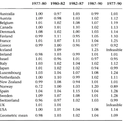
Norway, Australia and Denmark among the last seven. Although the quantity index in (10.9) is not designed to measure performance over time, examina-tion of the ranks pertaining to each year reveals the spectacular performance of France and Sweden, which raised their ranks from 12th to 1st position and from 18th to 5th, respectively. Greece, Israel, Norway, Ireland and Japan, on the other hand, seem to have lost their comparative advantage in the provi-sion of a healthy standard of living. The last column in Table 10.2 is reserved for the overall improvement in the human well-being index computed using (10.10). A breakdown of human improvement index for subperiods is also provided in Table 10.3.

An analysis of the overall improvement rate combined with observations on a year-to-year variation of the relative rankings of countries reveals fairly consistent results. For example, France and Sweden owe their quite spectac-ular climb with regard to their rank among the 22 countries to their rather high improvement rates (25 per cent and 28 per cent, respectively). Spain, on the other hand, maintains its top position among the countries because of its high overall improvement rate, an achievement shared with Sweden.

We also observe that countries showing deterioration in performance (like Greece, Japan, Switzerland and Norway) have also experienced a fall in their relative ranking. It is also useful note that a comparison of quantity indexes across time will not reveal much about overall improvement. With such a comparison, one would incorrectly conclude, for example, that Spain shows no improvement, whereas with its highest growth performance, it is, in fact, the country that boosts the distribution of human well-being index over time.4

Conclusions

This chapter, relying on an economic-theoretical approach to index num-bers, proposes a framework for incorporating environmental indicators to the measurement of human well-being. Furthermore, this study also introduces an improvement index which alleviates the well-known deficiency of across-time comparison of deprivation indexes. The benefit of the proposed index is that it does not require normative judgements in the selection of weights to aggregate over constituent indices. Instead, optimally chosen weights, within an activity analysis framework, are determined by the data. In developing the index which incorporates environmental indicators, due emphasis is put on production with negative externalities and directional distance functions -a very recent -an-alytic-al device - -are employed -as -a m-ajor tool to construct quantity indexes and improvement indexes. The improvement index is well grounded in the theory of productivity growth. The chapter also provides a numerical example of computations over 22 high income OECD countries to show that the indexes proposed are capable of differentiating variations in human well-being where more traditional indexes fail.

Osman Zaim 207 Notes

1. See Ivanova eta/. (1999), Anand and Ravallion (1993) and McGillivray (1991). 2. Shephard (1970) introduced the notion of weak disposability of outputs. 3. Shephard and Fare (1974) introduced this property.

4. See Zaim eta/. (2001) for details on the superiority of the improvement index in this study versus across-time comparison of deprivation indexes.

References

Anand, S. and M. Ravallion (1993) 'Human Development in Poor Countries: On the Role of Private Incomes and Public Services', Journal of Economic Perspectives, 7, 1: 133-50.

Chung, Y.H., R. Fare and S. Grosskopf (1997) 'Productivity and Undesirable Outputs: A Directional Distance Function Approach', Journal of Environmental Management, 51: 229-40.

Fare, R., S. Grosskopf and C.A.K. Lovell (1994) Production Frontiers (Cambridge: Cambridge University Press).

Fare, R. and D. Primont (1995) Multioutput Production and Duality: Theory and

Applica-tions (Boston: Kluwer).

Fisher, I. (1922) The Making of Index Numbers (Boston: Houghton Mifflin).

Grosskopf, S., S. Self and 0. Zaim (2002) 'To What Extent is the Efficiency of Public Health Expenditure Is Determined by the Status Health?', Paper presented at the AEA CSWEP Session 'Health and Disability Issues', January, Washington, DC.

Ivanova, 1., F.]. Arcelus and G. Srinivasan (1999) 'An Assessment of the Measurement Properties of Human Development Index', Social Indicators Research, 46: 57-179. Lasso de Ia Vega, M.C. and A.M. Urrutia (2001) 'HPDI: A Framework for Pollution

Sen-sitive Human Development Indicators', Environment, Development and Sustainability, 3, 3: 199-215.

McGillivray, M. (1991) 'The Human Development Index: Yet Another Redundant Composite Development Indicator?', World Development, 19, 10: 1461-8.

Nath, B., I. Talay and H. Tanrivermis (1998) 'Proposed Methodology for the Calculation

of Local Sustainability Indicator, in L. Hens, R.J. Borden, S. Suzuki and G. Caravello (eds), Research in Human Ecology: An Interdisciplinary Overview (Brussels: UVP-Press), 247-58.

Prescott-Allen, R. (2001) The Wellbeing of Nations: A Country-by-Country Index of Quality

of Life and the Environment (Covel, CA: Island Press).

Sen, A.K. (1976) 'Poverty an Ordinary Approach to Measurement', Econometrica, 44: 219-31.

Shephard, R.W. (1970) Theory of Cost and Production Functions (Princeton: Princeton University Press).

Shephard, R.W. and R. Fare (1974) 'The Law of Diminishing Returns', Zetschrift fiir

Nationa/Okonomie, 34: 69-90.

United Nations (UN) (2001) Sustainable Development Indicators. Available at: www. un.org/susdev

Zaim, 0., R. Fare and S. Grosskopf (2001) 'An Economic Approach to Achievement and Improvement Indexes', Social Indicators Research, 56 (1): 91-118.

Zheng, B. (1993) 'An Axiomatic Characterization of the Watts Poverty Index', Economics