Solution of electromagnetic scattering problems involving curved surfaces

^ Щ - i f д ;f··^ ^ í Г·'·

':'■-L V i N 'S C U í l V S I i S - J

SOLUTION OF ELECTROMAGNETIC SCATTERING

PROBLEMS INVOLVING CURVED SURFACES

A THESIS

SUBMITTED TO THE DEPARTM ENT OF ELECTRICAL AND

ELECTRONICS ENGINEERING

AND THE INSTITUTE OF ENGINEERING AND SCIENCES

OF BILKENT UNIVERSITY

IN PARTIAL FULFILLMENT OF THE REQUIREMENTS

FOR THE DEGREE OF M ASTER OF SCIENCE

5<or+£-l.

By

Kubilay Sertel June 1997

(ÀC 6 6 5

■S3

ía^-9-I certify that ía^-9-I have read this thesis and that in iny opinion it is fully adequate, in scope and in quality, as a thesis for the degree of Master of Science.

Asst. Prof. Dr. Levent Giirel(Supervisor)

I certify that I have read this thesis and that in my opinion it is fully adequate, in scope and in quality, as a thesis for the degree of Master of Science.

Assoc. Prof. Dr. M. îrşadi Aksun

I certify that I have read this thesis and that in my opinion it is fully adequate, in scope and in quality, as a thesis for the degree of Master of Science.

Prof. Dr. Ayhan Altıntaş

Approved for the Institute of Engineering and Sciences:

Prof. Dr. Mehmet Ban

ABSTRACT

SOLUTION OF ELECTROMAGNETIC SCATTERING

PROBLEMS INVOLVING CURVED SURFACES

Kubilay Sertel

M .S . in Electrical and Electronics Engineering Supervisor: A sst. Prof. Dr. Levent Gürel

June 1997

The method of moments (MoM) is an efficient technique for the solution of electromagnetic scattering problems. Problems encountered in real-life appli­ cations are often three dimensional and involve electrically large scatterers with complicated geometries. When the MoM is employed for the solution of these problems, the size of the resulting matrix equation is usually large. It is pos­ sible to reduce the size of the system of equations by improving the geometry modeling technique in the MoM algorithm. Another way of improving the effi­ ciency of the MoM is the fast multipole method (FM M ). The FMM reduces the computational complexity of the convensional MoM. The FMM has also lower memory-requirement complexity than the MoM. This facilitates the solution of larger problems on a given hardware in a shorter period of time. The com ­ bination of the FMM and the higher-order geometry modeling techniques is proposed for the efficient solution of large electromagnetic scattering problems involving three-dimensional, arbitrarily shaped, conducting suriace scatterers.

ÖZET

E Ğ R İ Y Ü Z E Y L E R İÇ E R E N E L E K T R O M A N Y E T İ K S A Ç IN IM P R O B L E M L E R İN İN Ç Ö Z Ü M Ü

Kııbilay Sertel

Elektrik ve Elektronik Mühendisliği Bölüm ü Yüksek Lisans Tez Yöneticisi: Y . Doç. Dr. Levent Gürel

Haziran 1997

Moment metodu (MoM) elektromanyetik saçınım problemlerinin çözümü için etkili bir 3Üntemdir. Günlük ha}^atta karşılaşılan saçınım problemleri çoğunlukla üç boyutludurlar ve elektriksel olarak büyük, karmaşık geometrili saçıcılar içerirler. Bu problemlerin çözümünde MoM kullanıldığında elde edilen matrisin boyutu genellikle büyüktür. Bu denklem sisteminin bo,yu- tıınu MoM algoritmasındaki geometri modellemesini iyileştirerek düşürmek mümkündür. M oM ’un etkinliğini arttırmanın başka bir yolu da hızlı multi- pol metodudur (FM M ). FMM bildik M oM ’un işlemsel karmaşıklığını düşürür. FMM için gereken bellek miktarının karmaşıklığı da MoA4 için gerekenden düşüktür. Bu, verilen bir donanım üzerinde daha büyük boyutlu problemlerin daha, kısa zamanda çözülebilmesini olanaklı kılar. FMM ve yüksek dereceli geometri modelleme tekniklerinin birleştirilmesi üç boyutlu, rastgele şekilli, iletken yüzey saçıcılarmm bulunduğu büyük elektromanyetik problemlerinin etkili çözümü için önerilmiştir.

ACKNOWLEDGMENTS

I would like to express my deepest gratitude to my supervisor Asst. Prof. Dr. Levent Gürel for his guidance, suggestions, and invaluable encouragement throughout the development of this thesis. I would like to thank to Assoc. Prof. Dr. M. İrşadi Aksun and Prof. Dr. Ayhan Altıntaş for reading and commenting on my thesis.

Special thanks go to I. Kürşat Şendur for his invaluable discussions and help in every step of this thesis. I would also like to thank to him, to Ertem Tuncel and to Uğur Oğuz for sharing hard times, day and night, in the office.

TABLE OF C O N TEN TS

1 Introduction 1

2 M oM and F M M 4

2.1 The Electric-Field intégral Equation .'l

2.2 Method of Monrents (>

2.3 Multipole I'ix|)a.iisions and FMM Formulation 9

2.3.1 Formulations for the F M M ... 11

2.3.2 Description of the FMM A lg o r ith m ... 12

2.3.3 Required Number of Multipoles and Directions... T5

2.3.4 Memory Requirements and Computational Complexity . 16

3 Geometry-Modeling Techniques 18

3.1 Parametric Space C u rv es... 19

3.3 Polynomial Interpolation S u rfaces... 23

3.3.1 Staircase A pp roxim ation ... 23

3.3.2 Flat Triangulations... 24

3.3.3 Quadratic Triangulations... 25

3.3.4 Biquadratic A pproxim ation s... 26

3.4 Free-Form S u rfa c e s... 27

3.4.1 Bezier Patches... 28

3.4.2 B-spline Surfaces 30 3.4.3 Nonuniform Rational B-Spline (NURBS) Surfaces . . . . 32

4 Basis Functions 34 4.1 Rooftop (RT) Basis F u n ctio n s... 35

4.2 Rao-VVilton-Gli.sson (RWG) Basis F u n c t io n s ... 36

4.3 Curved Rooftop (CRT) Basis F unctions... 36

Curv'ed RWG (CRWG) Basis Functions First-Order RT Basis Functions 5 Scattering from Canonical and Complicated Targets 47 5.1 Flat P a t c h ... 48

5.2 S p h e r e ... 69

5.2.1 Flat Triangulation with RWG BFs 70 5.2.2 E.xact Model with CRWG B F s ... 71

5.2.3 Exact Model with CRT B F s ... 74

5.2.4 Quadratic Triangulation with CRWG BFs ... 77

5.2.5 Bezier-Patch Model with CRT B F s ... 83

5.2.6 Comparison of Different Modeling Schem es... 86

5.3 M is s ile ... 94

6 Conclusions 100 A Evaluation of the M oM Matrix Elements 103 A.I Singular Integrals Appearing in the F orm ulation...104

.A.2 Technicpies to Annihilate the S in g u la rity ... 107

.A.2.1 For Triangular Subdomains ... 108

A .2.2 For Square Subdomains ... I l l A.3 .\himerical Integration ...122

LIST OF FIGURES

2.1 The basic geometiy illustrating the relationship between x ,x ', r, and d .... 10

2.2 The geometry construction used in FMM formulations, illustrat­ ing the relation between source point, field point and the group

centers. 11

2..·] Illustrcition of the FMM strategy... 14

.3.1 A parametric space curve is a vector function of a parameter u. 19

3.2 A generic Bezier curve and its defining polygon... 21

3.3 .4n aircraft approximated by a mesh of rectangular cells. (Re­

produced from [18].) 24

3.4 Sphere approximated by a mesh of flat triangles. The triangu­

lation is performed by MSC/ARIES. 25

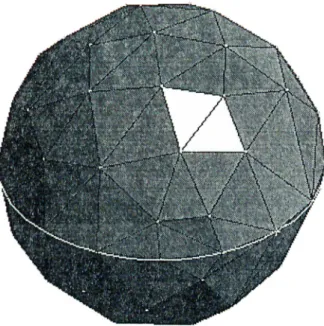
3.5 Spliere approximated by a mesh of 6-point quadratic triangles. The triangulation is performed by M SC/ARIES... 26

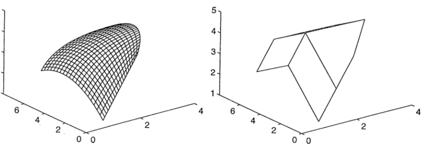
3.6 Sphere approximated by a mesh of 9-point biquadratic rectan­ gular patches. Reproduced f r o m ... 27

3.7 Tensor product Bezier surface and its defining pol}^gon net. 30

3.8 A yatch hull defined as a B-spline surface, the defining polygon net and the parametric representation. (Reproduced form [16].) 31

3.9 Sphere generated as a rational B-spline surface, (a) Offset circle and defining polygon; (b) circle of revolution and defining poly­ gon; (c) defining polygon net and sphere. (Reproduced from [16].) 33

4.1 Rooftop basis function defined a pair of flat rectangular regions. 35

4.2 Rao-W ilton-Glisson Ijasis function on a pair of flat triangular

regions. 36

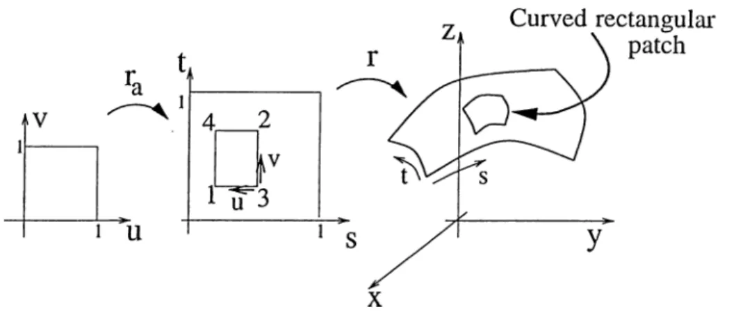
4.3 Composite mapping of the parametric unit sciuarc on the real

curved surface. 38

4.4 C-RT BF defined on the parametric space. 39

4.5 CRWG BF defined on the unit triangle in the parametric space. 42

4.6 First-order rooftop basis functions defined on the (t/.,n) para­

metric space. 45

5.1 Flat PEC patch illuminated by a plane wave.

5.2 Discretization of the flat patch.

19

5.3 The induced current and charge densities on the flat patch. The patch is discretized into 10 x 10 divisions and the RT BFs on the internal edges are used for the expansion, (a) Magnitude of the copolar induced current, (b) Magnitude of the crosspolar current, (c) Real part of the divergence of the induced current. (d) Imaginary part of the divergence of the induced current. The current results are normalized with the magnitude of the incident magnetic field, and the divergence of the current is pre­ sented as the charge distribution... 51

5.4 The induced current and charge densities on the flat patch. The patch is triangulated into 200 subdomains and the RWG BFs on the internal edges are used for the expansion, (a) Magnitude of the copolar induced current, (b) Magnitude of the crosspolar current, (c) Real part of the divergence of the induced current, (d) Imaginary part of the divergence of the induced current. The current results cire normalized with the magnitude of the incident magnetic field, and the divergence of the current is pre­ sented as the charge distribution... 53

5.5 The induced current and charge densities on the flat patch. The patch is discretized into 20 x 20 divisions and the RT BFs on the internal edges are used for the expansion, (a) Magnitude of the copolar induced current, (b) Magnitude of the crosspolar current, (c) Real part of the divergence of the induced current. (d) Imaginary part of the divergence of the induced current. The current results are normalized with the magnitude of the incident magnetic field, and the divergence of the current is pre­ sented as the charge distribution... 54

5.G The induced current and charge densities on the flat patch. The patch is discretized into 10 x 10 divisions and two LinRT BFs on the internal edges are used lor the expansion. Transverse continuity is imposed at each internal vertex, (a) Magnitude of tlie copolar induced current. (1)) iNlagiiitucle of the crosspolar current, (c) Real part of the divergence of the induced current. (cl) Imaginary part of the divergence of the induced current. The current results are normalized with the mcignitude of the incident magnetic field, and the divergence of the current is pre- •sented as the charge distribution... 56

5.7 The induced current and charge densities on the flat patch. The patch is discretized into 20 x 20 divisions and two LinRT BFs on the internal edges are used for the expansion. Transverse continuity is imposed at each internal vertex, (a) Magnitude of the copolar induced current, (b) Magnitude of the crosspolar current, (c) Real part of the divergence of the induced current. (d) Imaginary part of the divergence of the induced current. The current results are normalized with the magnitude of the incident magnetic field, and the divergence of the current is pre­ sented as the charge distribution... 57

5.8 The induced current and charge densities on the flat ¡Datch. The patch is discretized into 10 x 10 divisions and two LinRT BFs on the internal edges are used for the expansion, (a) Magnitude of the copolar induced current. (1:)) Magnitude of tlie crosspolar current, (c) Real part of the di\’crgencc of the induced current, (d) Imaginary part of the divergence of the induced current. The current results are normedized with the magnitude of the incident magnetic field, and the divergence of the current is pre­ sented as the charge distribution... 58

5.9 The induced current and charge densities on the flat patch. The patch is discretized into 20 x 20 divisions and two LinRT BFs on the internal edges are used for the expansion, (a) Magnitude of the copolar induced current, (b) Magnitude of the crosspolar current, (c) Real part of the divergence of the induced current, (d) Imaginary part of the divergence of the induced current. The current results are normalized with the magnitude of the incident magnetic field, and the divergence of the current is pre­ sented as the charge distribution...

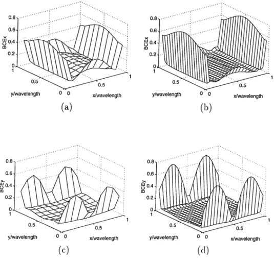
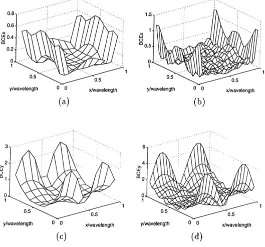
5.10 Boundary-condition error on the flat patch. The solution is ob­ tained using the RT BFs. (a) Copolar BCE for 10 x 10 discretiza­ tion. (b) Copolar BCE for 20 X 20 discretization, (c) Crosspolar BCE for 10 X 10 discretization, (d) Crosspolar BCE lor 20 x 20 discretization...

5.11 Boundary-condition error on the flat patch. The solution is ob­ tained using the transversely continuous LinRT BFs. (a) Copo- lar BCE for 10 x 10 discretization, (b) Copolar BCE for 20 x 20 discretization, (c) Crosspolar BCE for 10 x 10 discretization, (d) Crosspolar BCE for 20 x 20 discretization...

59

60

61

5.12 Boundary-condition error on the flat patch. The solution is ob­ tained using the LinRT BFs. (a) Copolar BCE lor 10 x 10 discretization, (b) Copolar BCE for 20 x 20 discretization, (c) Crosspolar BCE for 10 x 10 discretization, (d) Crosspolar

5.13 (a) Magnitude of the copolar induced current on a A x A flat patch, (b) Magnitude of the crosspolar induced current on a A x A flat patch. The color plots are generated using the M SC/ARIES. 65

5.14 Bistatic RCS of a 2A x 2A flat patch. — 15 x 15 division with 420 RT BFs, — MSC/ARIES triangulation with 560 RVVG BFs. 65

5.15 Timing comparisons of the MoM and the FMAl. (a) The matri.x solution times using the MoM with LU decomposition, the MoM with CGS, and the EMM with CCS , (b) The problem solution times using the MoM with LU decomposition, the MoM with CGS, and the EMM with C G S ... 66

5.16 CPU time consumed per one iteration of MoAl anf P'MM algo­ rithms. The iterative solution method is CGS. 66

5.17 .Appro.ximate memory requirements of the MoM and the F.MM

algorithms. 67

5.18 Validations of the EMM solutions, (a) Bistatic R.CS of a 2A x 2A flat patch using 736 CRVVG BFs, — the MoM solution, — the EMM solution, (b) Bistatic RCS of a 2A x 2A flat patch using 760 CRT BFs, — the MoM solution, — the EMM solution. . . 67

5.19 Bistatic RCS of a lOA x lOA flat patch. — 65 x 65 division with 8320 RT BFs, — M SC/ARIES triangulation with 8008 RWG BFs... 68

5.21 Flat triangulation of the sphere. 71

5.22 Magnitude of the surface current induced on the 0.2A-radius sphere. Flat triangulation of the sphere is used with the flat RWG basis functions. The results are normalized with the mag­ nitude of incident magnetic field and are given on the three principle cuts of the sphere for different discretizations and dif­ ferent numbers of unknowns. — Mie series, • • • 7 x 8 divisions and 144 unknowns, — · — 9 x 10 divisions and 240 unknowns,

11 X 16 divisions and 480 unknowns... 72

5.23 Magnitude of the electric field scattered by the 0.2A-radius sphere. Flat triangulation of the sphere is used with the flat RWG basis functions. The results are given on the three princi­ ple cuts of the sphere for different discretizations and different numbers of unknowns. — Mie series. · · · 7 x 8 divisions and 1 11 unknowns,--- 9 X 10 divisions and 210 unknowns, — 11 x 16

divisions and 480 unknowns... 73

5.24 Magnitude of the surface current induced on the 0.2A-radius sjDhere. Curved triangulation of the sphere is used with the CRWG basis functions. The results are normalized witli the magnitude of incident magnetic field and are given on the three principle cuts of the sphere for different discretizations and dil- fereiit numbers of unknowns. — iMie series, • • • 7 x 8 divisions and 144 unknowns, ·— · — 9 x 10 divisions and 210 unknowns,

5.25 Magnitude of the electric field scattered by the 0.2A-radius sphere. Curved triangulation of the sphere is used with the CRWG basis functions. The results are given on the three prin­ ciple cuts of the sphere for different discretizations and different numbers of unknowns. — Mie series, •••7x8 divisions and 144 unknow ns,--- 9 X 10 divisions and 240 unknowns, — 11 x 16

divisions and 480 unknowns... 76

5.26 Rooftop basis and testing functions on the sphere. I i

5.27 Magnitude of the surface current induced on the 0.2A-radius sphere. Curved rectangular meshing of the sphere is used with the CRT basis functions. The results are normalized with the magnitude of incident magnetic field and are given on the three principle cuts of the sphere for different discretizations and dif- fereait numbers of unknowns. — Mie series, · · - 5 x 6 divisions and 54 unknowns, — •— 7 x 8 divisions and 104 unknowns, —

9 X 18 divisions and 306 unknowns... 78

5.28 Magnitude of the electric field scattered by the 0.2A radius sphere. Curved rectangular meshing of the sphere is used with the CRT basis functions. The results are given on the three principle cuts of the sphere for different discretizations and dif­ ferent numbers of unknowns. — Mie series, · · · 5 x 6 divisions and 54 unknowns, ^ · — 7 x 8 divisions and 104 unknowns,----9 X 18 divisions and 306 unknowns... 79

5.29 Magnitude of the induced surface current on a 0.2A-radius sphere. The sphere is discretized using quadratic triangles and the EFIE is solved using the CRWG BFs defined on these tri­ angular subdomains. The color plot was generated using the M SC /A R IE S... SO

5.30 Magnitude of the electric field scattered the 0.2A-radius sphere. Curved triangulation of the sphere, obtained from the M SC/ARIES, is used with the CRWG BFs. The results are given on the three principle cuts of the sphere. — Mie series, • · · 156 curved RWG B F s ,--- 318 curved RWG BFs... 81

5.31 Magnitude of the electric field scattered l)y the 0.5A-ra.dius sphere. Curved triangulation of the si:>here, obtained from the M SC/ARIES, is used with the CRWG basis functions. The re­ sults are given on the three principle cuts of the sphere. — iMie series, ··· 480 curved RWG BFs, — · — 831 curved RWG BFs,

1020 curved RWG BFs... 82

5.32 Magnitude of the electric field scattered by the 0.2A-radius sphere. 8-patch Bezier model of the sphere is used with the CRT BFs. The results are given on the three principle cuts of the sphere. — Mie series, · ■ · 132 curved RT BFs, — · — 240 curved RT BFs... 84

5.33 Magnitude of the electric field by scattered the 0.5A-radius sphere. 8-patch Bezier model of the sphere is used with the CRT BFs. The results are given on the three principle cuts of the sphere. — Mie series, · · · 552 curved RT BFs, — · — 756 curved RT BFs, — · — 992 curved RT BFs... 85

5.34 Magnitude of the surface current induced on the 0.5A-radius sphere. Flat-triangulation, curved-triangulation, and curved- rectangular meshing of the sphere are used with the RWG, the CRWG, and the CRT BFs, respectively. The results are nor­ malized with the magnitude of incident magnetic field and are given on the three principle cuts of the sphere. — Mie series, · · · 11 X 16 divisions and 660 flat RWG B F s .--- 11 x 16 divisions and 660 curved RWG B F s ,---- 11 x 22 divisions and 462 curved

RT BFs... 87

5.35 Magnitude of the electric field scattered by the 0.5A-radius sphere. Flat-triangulation, curved-triangulation, and curved- rectangular meshing of the sphere are used with the RWG, the CRWG, and CRT BFs respectivel,y. The results are given on the three principle cuts of the sphere. — Mie series, •••11x16 divisions and 660 flat RWG BFs. - · - 11 x 16 divisions and 660 curved RWG B F s ,---- 11 x 22 divisions and 162 curved RT BFs...

5.36 Comparison of the different geometry models used in the com ­ putation of the magnitude of the electric field scattered by the 0.2A-radius sphere. Curved triangulation of the sphere, obtained from the M SC/ARIES, is used with the CRVVG BFs and the 8- patch Bezier model of the sphere is used with the CRT BFs. The results are given on the three princii^le cuts of the sphere. — Mie series, · · · 156 curved RWG BFs, — 132 curved RT BFs. 90

5.37 Comparison of the different geometry models used in the com ­ putation of the magnitude of the electric field scattered by the 0.5A-radius sphere. Curved triangulation of the sphere, obtained from the MSC/ARIES is used with the CRWG BFs and 8-patch Bezier model of the sphere is used with the CRT BFs. The re­ sults are given on the three principle cuts of the sphere. — Mie series, · · · 480 curved RWG BFs. — 552 curved RT BFs... 91

5.38 Maximum difference in the far-field solutions using different ge­ ometry models of the sphere... 92

5.39 Norm of the difference in the far-field solutions using different

geometry models of the sphere. 93

5.40 Validations of the FMM solutions, (a) Bistatic RCS of a 0.5A-radius sphere using 480 CRWG BFs, — the MoM solu tion ,----the FMM solution, (b) Bistatic RCS of a. 0.5A radius sphere using 380 CRT BFs, — the MoM solution, — the FMM solution. 94

5.11 Quadratic triangular mesh of the missile generated using tlie MSC/ARIES... 9-5

5.42 Magnitude of the induced surface current on a 6-meter long mis­ sile at 100 MHz. The missile is discretized using quadratic tri­ angles and the EFIE is solved using the CRWG BFs defined on these triangular subdomains. The color plot is generated using the M SC/ARIES... 96

0.43 Comparison of the bistatic RCS of the 6-meter long missile at 100 MHz. Curved and flat triangulations of the missile, obtained from the M SC/ARIES, is used with the CRWG BFs and flat- RWG BFs respectively, and 34-patch Bezier model of the missile is used with the CRT BFs. The results are given on x-z plane, where the main wings of the missile are located. — 1053 flat- RWG BFs, — 1053 CRWG BFs, · ■ · 1088 CRT BFs... 97

5.44 Comparison of the bistatic RCS of the 6-meter long missile at 200 .MHz. Curved and flat triangulation of the missile, obtained from the .MSC/ARIES, is used with the CRWG BFs and Ha.t- RWG BFs respectively, and 34-patch Bezier model of the missile is used with the CRT BFs. The results are given on x-z plane, where the main wings of the missile are located. — 2058 flat- RWG BFs, — 2058 CRWG BFs, · · · 2448 CRT BFs... 98

5.45 Comparison of the bistatic RCS of the 6-meter long missile at 300 MHz. Curved and flat triangulation of the missile, obtained from the hiSC/ARIES, is used Avith the CRWG BFs and flat- RWG BFs respectively, and 34-patch Bezier model of the missile is used with the CRT BFs. The results are given on x-z plane, where the main wings of the missile are located. — 7713 flat- RWG BFs, — 6213 CRWG BFs, · · · 4352 CRT B F s , ... 99

Л.1 Parametric mapping of the unit triangle to the curved triangle in real space... 109

Л.2 Subdivision of the parametric unit triangle for singularity anni­ hilation...110

A.3 Mapping of sub-triangle 1...110

A. l Mapping of sub-triangle 2...110

A .5 Mapping of sub-triangle 3...I l l

A .6 Mapping defined to annihilate the singularity at the origin. . . . 112

A .7 Mapping of Method II... 113

y\.S Mapping of the parametric unit square to a curved rectangular ... 114

A .9 Subdivision of the unit square into sub-triangles... 115

A .11 The subdivision of the unit square for Method III... 118

A. 12 The transformation for the first subdomain... ... . 118

Chapter 1

Introduction

Solution techniques based on the surface integral equations (SIEs) are widely used in computational electromagnetics. Formulations employing SIEs ex^press the unknown function on the defining surface of the i^roblem geometry. Thus, both t he surface a.nd tlie unknown function defined on it ha.ve to be accurately represented in the solution algorithm.

Real-life electromagnetic scattering problems are often three dimensional and involve arbitrary geometries. Formulations of these problems can not be based on the arbitrary geometries of the problems, instead, the geometries are approximated by various mathematical models that are easier to work with . Approximating the problem geometry by polynomial suljsections is b('coming widely used in most of the numerical solution teclmi([ues, such as the finite element method (FEM) and the method of moments (MoM) [1, 2]. d'he MoM, which will be explained in detail in Chapter 2, provides a flexible and powerful formulation for the solution of electromagnetic scattering and

radiation problems.

Canonical geometries such as spherical, cylindrical, and conical surfaces can be exactly modeled. Arbitrarily curved surfaces can be accuratelj'^ modeled us­ ing a mesh of biquadratic, bicubic, or higher-order polynomial surface patches. Non-uniform rational B-spline (NURBS) surfaces and Bézier^ patches can also be used for the same purpose. NURBS surfaces are powerful modeling tools that are widel}^ used in computer-aided graphical design (C AG D ) applications. Hence, the representations of most bodies fabricated by using automated ma­ chining processes are based on NURBS meshes. Therefore, if the geometry of the scatterer is represented by NURBS surfaces in the electromagnetic scatter­ ing code, the output data of a CAGD tool can be directly used as the input of the code without inducing any geometry-modeling error in the solution.

In this thesis, a general formulation of the MoM for electromagnetic scatter­ ing problems involving arbitrarily sliaped, conducting scatterers will be given. The limitations of this method will be mentioned and ways to overcome these limitations will be investigated.

The effect of using different techniques to approximate the problem ge­ ometry on the solution will be investigated. Comparisons of solutions different geometry-modeling techniques will be given. It will be shown that better geom­ etry models improve the solution accuracy and reduce the size of the resulting matrix equation. Comparisons of results obtained using different basis hinc- tions in the Mohi expansion will also be given, and it will be sliown that the accuracy of the solution heavily depends on the geometry-modeling scheme rather than the type of the basis functions.

The basis functions used in the expansion of the unknown function in the MoM formulations are defined to be conformal with the surface representation and are “curved” generalizations of the piecewise linear basis functions defined on flat rectangular domains (rooftops) [3, 2] and flat triangular domains (due to Rao, Wilton and Glisson) [1, 4]. Issues concerning the numerical computa­ tion of the singular and nonsingular integrals arising in the formulations using différent surface representations and different basis functions will be addressed.

A general formulation of the fast multipole method (FM M ) [5, 6, 7] for electromagnetic scattering problems will also be given. The performance of FMM will be investigated. Both the eificency and the accurac}'^ of the FMM wilt be demonstrated by comparing the FMM solutions to the MoM and closed- form solutions for some sample problems. Thus, the combination of the FMM and accurate geometry-modelling techniques will be proposed for the efficient solution of real-life electromagnetic scattering ])roblems.

Chapter 2

M oM and F M M

The MoM is a well-known technique for obtaining approximate solutions of integral, differential, and integro-differential equations arising in various areas of basic and applied sciences [8]. The equation to be solved is converted into a matrix equation by applying the standard MoM procedure. 'I'lie procedure is outlined in Section 2.2. This matrix ecpiation is then solved either by Gaussian elimination (GE) or by an iterative solution scheme such as tlie conjugate gradient method (CGM ). GE requires 0{N^) operations for the solution of an N X N system. An iterative solver would require 0{N^) operations per iteration. As N gets larger, these high complexities limit the performance and applicability of the MoM.

Eor electromagnetic scattering and radiation problems, the EMM can be utilized to reduce the O(N^) complexity of an iterative solver to (9(yV'"’ ). This is accomplished by calculating the matrix-vector product in a last and indirect way at iteration of the iterative solver. This chapter outlines the MoM and the

FMM as they are applied to electromagnetic scattering problems.

2.1

The Electric-Field Integral Equation

fiased on Maxwell’s equations, one way of formulating the electromagnetic scattering problems involving open or closed conducting surfaces is the so called electric-field-integral-equation (EFIE) formulation. Maxwell’s equations in the frequency domain can be manipulated to obtain the a equation,

V2E(r) + A:^E(r) = -¿o ;/iJ (r), (₂.₁)

in free space with time convension. The solution to this equation is given by

E(r) = -iwfi [ d e 'G (r .r ') · J (r'). J V

In the above.

G (r ,r ') =

is the dyadic Green’s function and

i _ T v v

(2.2)

(2.3)

.9(r,i·') =

r — r (2..I)

is the scalar Green’s function that satishes the scalar wave equation

(V2 + A:2)^(r,r') = ^ (i'-r0 ·

For a giv'en source distribution J (r), the electric field radiated by tliat source distribution can be calculated using Eq. (2.2).

For conducting objects, the EFIE is given by

I.

2

6

Equation 2.6 is the statement of the boundary condition on the tangential component of the electric held on a conducting surface. The vector denoted b}'^ t is any unit tangent vector on the surface s of the scatterer, and E '(r ) is an impressed held which excites the system.

2.2

Method of Moments

The EFIE for the unknown electric current density J (r) on the conducting sur­ face induced l)y an incident wave is discretized using the MoM tecluiic|ue. Tlie induced surface current is approximated by a sum of N known basis functions {jn (i')} as

N

J(··) “ (2.8)

ii = l

The EFIE thus becomes

N . r 1

/1=1 ^ ^

,ikR _Atti

-— d s ' - -— L- E’ { v ) ^ Q (2.9)

R An;

Hence tlie proldem is reduced to hnding a. set of n „’s tliat minimizes the error in Eq. (2.9).

is converted into a system of equations, whose solution minimizes the boundary- condition error in the average sense. The system of equations obtained is,

N y ^ Zmn^n — Fm·) — 1; 2, . . . , A^, n=l where and dst„,(r) · ds' [j„(r ') + ^ V ' · j„ ( r ') V AkR R = m Airi krj J^dst,n{i') ■ E*(r). (2 .1 0 ) (2.1 1) (2 .1 2 )

Hence, the actual problem of finding the induced surface current J (r) is reduced to finding N coefficients of expansion of Eq. (2.8) as the solution of Eq. (2.10).

The expansion functions should be chosen so that their combination in Eq. (2.8) is capable of representing the unknown current density J (r) suffi­ ciently well. Quite powerful basis functions (BFs) exist in the literature for the expansion of induced surface current in scattering problems, most common ones being the RWG^ BFs supported on planar triangular subdomains [1] and rooftop (RT) BFs supported on planar rectangular subdomains [3]. For curved subdomains, generalizations of flat RWG BFs and flat RT BFs that are confor­ mal with the curved surface they are defined on [2, 4] are used. The definitions of these basis functions will be given in Chapter 4. Entire-domain BFs are also used in the MoM formulations, but will not be mentioned here. It should be noted that the BFs chosen for the approximation of the current J (r) should also be capable of providing a consistent approximation of the surface charge

of providing a consistent approximation of the surface charge p(r), which is related to the current through the continuity equation [9]

V · J (r) — ¿a>p(r) = 0. (2.13)

The choice of testing functions is also arbitrary but some methods are more popular in practice. If the testing functions are chosen to l)e the same as the basis functions, the method is called Galerkin’s method. It can be pro\ en that Galerkin’s method is equivalent to Rayleigh-Ritz variational method [8]. When the error is constrained to be satisfied on a set of discrete points on tlie scat- terer, which corresj^onds to choosing testing functions to be delta, functions on the scatterer surface, the method is named as point matching, and when they are chosen to be pulse functions defined over the subdomains of the geometry, the method is called collocation by subdomains. Wlien the testing functions are chosen to be the complex conjugates of the basis functions, the formulation results in the minimization of the square of llie error, 'riiroughout this thesis. Cîalerkin’s method is used. In addition to being a variational method, another advantage of the Galerkin’s method is that the resultant MoM matrix is sym­ metric. Therefore, one need only compute and store half of the MoM matrix Zmn- This is also an important consideration for the choice of the solution algorithm.

Direct application of the MoM requires the computation of N'^ double sur­ face integrals appearing in Eq. (2.11) as the elements of tlie resulting MoM matrix. Solution of this system of equations by Gaussian elimination requires 0(N'-^) operations. Iterative solvers require 0(N'^) operations per iteration. The niem oiy requirement ol the MoM is also 0{N ^). 1 his large order lor stoi’cige limits the size of the problem that can be solved on a given hardware.

and the high operation cost poses a limit to the size of problems that can be solved in a practically acceptable period of time. For these reasons, the FMM is proposed [5, 6, 7, 10], which requires less memory and CPU time for the solution of large problems.

2.3

Multipole Expansions and F M M Formu­

lation

Direct application of the MoM requires the computation of double surface integrals appearing as the elements of the resultant MoM matrix and 0{N'^) operations per iteration for the iterative solution of the resulting system of c(|uations. A clever way to overcome the difficulties arising from these large storage and computation complexities is used in the FMM. The FMM is de\xil- oped using two elementary identities. The first is tlie expansion of tlie scalar Green’s function appearing in Eq. (2.11) as

(2.14) |r + d|

wliich is a form of Gegenbauer’s addition theorem [11]. Here ji is the spherical Bessel function, is the spherical Hankel function of the first kind, P\ is the Legendre polynolmial, and d < r is the condition tor the validy of the ex|)ansion. In the FMM formulations of scattering problems, where the source point is denoted by x' and the observation point by x, r will be chosen to lie close to X — x ' so that d will be small as depicted in Fig. 2.1. The second identity is the expansion of jtPi product appearing in Eq. 2.11 as a. sum ot

X

P’igure 2.1: The basic geometiy illustrating the relationship between x ,x ', and d.

propagating plane waves [11]:

4ni‘ji{kd)Pi{d · — j d^ke'^'^Pi{k · r). (2.15)

The Green’s function in Eq. (2.14) can be rewritten using Eq. (2.15) as

ih r ^

| 7 T d i = s / + \ )h f\ kr)p,(k ■ f), (2.16)

where the orders of summation and integration are interchanged. The idea, of the EMM is that the function

TiXkr, k ■

f) = Y^Cll + l)kl‘\kr}Pi(k ■

can be computed for various values of kr which is independent of kd. The series is truncated at the Lth term in numerical practice. The number of terms kept, L + 1, depends on the maximum allowed value of kd, as well as the desired accuracy. The choice of L will be mentioned later. Using Eq. 2.16, Eq. (2.14) Irecomes

^ifc|r+d| ¡1^.

|r + d| Itt

J

Figure 2.2: The geometry construction used in FMM formulations, illustrating the relation between source point, field point and the group centers.

2.3.1

Formulations for the F M M

The direct path from a source point to the field point can be decomposed into three parts as in Fig. 2.2, where

^ji — ^ jm T ^mm' I'iiu'· (2.19) The idea to be noted is that the same path will be used for all source point in cluster m' to translate their field to all observation points in cluster m. Fquation (2.1G) can be rewritten as

(

2

20

rji

and the Green’s function becomes

1 I --- V V ' k:^ ^ikTji rji

«

[l - ^V V']

[I -

(2.21)

Using the above equations, a matrix element as in Eq. (2.11) is approxi­ mated by

Z,nn = I f/^t„,(r) · 2,

[jn(r') + ^ V ' · j„(r')V

.ikR

(2-22)

where

V/rnAh = l i - k k j - t j ( r ^, n) (2.23)

are the Fourier transforms of the basis and testing functions, respectively, and the superscript denotes complex conjugation.

The FMM is proposed for the acceleration of the matrix-vector product computed at each iteration of an iterative solution scheme, like the conjugate gradient method, emplo3^ed for the solution of the resultant matrix equation. The algorithm is outlined in the next subsection.

2.3.2

Description of the F M M Algorithm

Normally the matrix-vector product at each iteration of an iterative solver would require 0{N^) multiplications for the solution of an N x N system of equations. Emploj'ing the algorithm below, it is possible to reduce this order to 0{N^"'). The FMM algortihm can be described as follows:

1. The N basis functions are divided into M localized groups (clusters), each containing about N/Al basis functions.

2. For groups tliat are distant to each other, the translation functions of Eq. (2.17) for each i)air of distant groups are calculated tor a predeter­ mined .set of k directions. Choice of this set ol k directions and the

choice of truncation limit for the series will be mentioned later. This re­ quires 0 { K L M { M — G)) computations, where G is the average number of nearby groups to each group, K is the number of k directions, and L is the number of terms kept in Eq. (2.17).

3. The Fourier transforms of each basis function are computed for the pre­ determined set of k directions. This step requires 0 { K N ) computation.

4. For groups that are near or close to each other (the closeness is defined in the sense that either Eq. (2.14) is not valid or the computation requires too maii}'^ terms of the series to be considered for at least one pair of source and field points), a sparse matrix denoted by Z' is constructed, with direct computation of matrix elements using Eq. (2.11). This step requires 0 { G{ Nj M) ^ M) computations.

5. The K M quantities called aggregations

Sm'(^) — (2.24)

which represent the far field of each group ???/ are computed using the precomputed Fourier transforms. This step requires 0 { K N ) operations.

6. The K M quantities called translations

g.,n{k) = E'Tnгr,г4)SnAk) (2.25)

representing the Fourier components of the field in the neigliborhood ol group ???., generated by the sources in the groups that are not nearby are computed next. This step requires 0 {K M {M — G')) operations using the precomputed values of T,nm'{A·

group m

7. Finally, the disaggregations of the fields of all sources in distant groups are computed from the group centers to the testing functions and added to the sparse matrix-vector product, which represents the testing of the field generated by the sources in nearby groups. This computation can be expressed as

B..« = E 2 , + /

<PkV,„iCk

m'i

Figure 2.3 depicts the three main steps of the algorithm.

L is proportional to the size D, the maximum of the diameters of all groups, and K = 2T^ is approximately proportional to D^. Since is approximately proportional to Nf M, the number of unknowns in a cluster (for surlace scat- terers), computation of the vector B in Ecp 2.26 reciuires aNM + h.\^/M operations, wliere a and h are machine-dependent constants. Ihis total opera­ tion count is minimized by choosing M — \Jl)Nla^ and the result is an

Extensions of the EMM that can further reduce this computational com ­ plexity exist in the literature. Multilevel EMM [12], which extends the EMM strategy with multilevel grouping, can reduce the computational complex­ ity to 0 { N log N). Raj'^-propagation fast multipole algorithm (R PFM A ) [13, 14] reduces the complexity to The fast far-held approximation (FAFFA) [15] also results in an algorithm. Among the methods men­ tioned above, on 1}'^ the FMM is implemented in this work. The implemenations of the extensions of the FMM mentioned above are among the future work that can be carried on on this subject.

2.3.3

Required Number of Multipoles and Directions

In the numerical implementation of the FMM, the series in Eq. (2.14) is eval­ uated using a finite number of terms. The number of terms that must be ('\aluated is cliosen so that the exj^ansion converges to the desired accuracy. For I < z the Bessel functions jt(z) and h\^\z) are nearly constant in magni­ tude, and for / > z, ji{z) decays rapidly and h\^\z) grows rapidly. Therefore, tlie truncation limit cannot be chosen to be much larger than kr^m'·, since the numerical evaluation of the integral in Eq. (2.16) will cause inaccuracies due to the oscillatory integrand. A semi-empirical fit given in [7] to the number of multipoles recjuired for single precision (32-bit reals) is

Ls{kD) = FD + 51n(A:D + Tr), (2.27)

where D > l/k is the maximum group diameter. For double precision, the estimate is

If the value of L dictated by the above formula used exceeds kr-mm'·, then the groujDS must be considered as neighboring, and their interaction must be included in the sparse near-field matrix ^^n·

The integral in Eq. (2.16) must be evaluated using a quadrature rule that would provide sufficient accurac}'^ in the result. A simj^le method for determin­ ing the sampling points is to pick polar angles 9 such that they are zeros of Pi[cosO)^ and azimuthal angles (f> to be 2L equally spaced points so that the azimuthal variation is sampled at the Nyquist rate. For this choice, K = 2L^.

2.3.4

M em ory Requirements and Computational Com ­

plexity

The memory required for the FMM can be considered in two parts, the sparse- matrix storage and tlic fidVllVl elements’ storage. The storage of the sparse Z' matrix requires 0{N^ fM ) memory locations. The FMM aggregations need 0 { K N ) memory locations, and the FMM translations need 0 { K L M^ ) memory locations. Hence the total memory storage needed is 0 { N ‘^fM) + 0 { K N ) -k 0 { K L h P ) . Using the proportionalities K oc T'·^, oc Nf M, and L oc D, this expression can be simplified to C\{N^jM) -T C

2

-2

('2

The computational complexity of the FMM can be determined by count­ ing the number of floating-point operations required at each step ol tlie al­ gorithm. The aggregation step requires MK N / M = R N operations. Tlie

translation step requires KNP oi^erations with the precomputed KM^ val­ ues of the translation function given in Eq. (2.17). The disaggregations require M K N /M = K N operations, and finally the sparse matrix-vector product requires N^/M operations. Using the proportionalities K oc

(X lY/M, and L X D, the total cost of the matrix-vector product is found as 0 { N M ) -j- 0 { N ‘^fM). This can be minimized by choosing M — \/N and the result is an algorithm. The memory required for the EMM also becomes Both the operation cost and the memory requirement of the EMM is less than those of standart MoM formulation for problem sizes larger than 1000, which makes the EMM more suitable for the solution of large problems.

Chapter 3

Geometry-Modeling Techniques

Real-life electromagnetic scattering problems, almost always, involve electri­ cally large scatterers with complicated geometries. In the formulation of scat­ tering problems involving three-dimensional arbitrarily curved scatterers, the gt'oinetry of iJie scatterer has to be appro.xdmated. Various geometry a.ppro.xi- mation and modeling techniques e.xist for this purpose [16, 17], some of which are presented in this chapter.

As the electrical size of a geometry gets larger, the size of the problem increases and the CPU time consumed and the memory required to obtain the solution grows rapidly. Hence, the maximum size of the problem that can l)e soKed on a given hardware is limited by these two (actors. Using l^etter geometry models for the scatterers, it is possible to reduce the size oi the ])roblem. As an introduction to the mathematical Isackground ot tlie subject of better modeling, parametric space curves will ]>e mentioned in the next section.

Figure 3.1: A parametric space curve is a vector function of a parameter u.

3.1

Parametric Space Curves

A general 3-D parametric curve in space (Fig. 3.1) is written of the form f(u ), where f is a vector containing the Cartesian coordinates of the point on tlie s|)a.cc curve having the i^arameter \alue u.

If f(?i) is an 7?.th degree polynomial function of u liaving a. set of \'ectors { a o ,a i ,. . . ,a „ } as coefficients, i.e.,

2=0

(3.1)

then one can specify the whole curve uniquely with this set of coefficients. Alternatively, one can specify another set of n + 1 points through which the y/th degree parametric polynomial curve is supposed to pass.

There are other methods of specifying an 7ith degree parametric polynomial curve, one of the most popular being the so called Bezier cur\'es [17]. /V Bezier curve is specified by an alternative set of points whicli is called the defining polygon. The shape of the actual cur\-e closely follows the sliape of the defining

polygon. Figure 3.2 shows a generic third-order Bezier curve and its defining polygon.

These curves have the following nice properties:

• The degree of the polynomial defining the curve segment is one less than the number of defining polygon points.

• Idle curve generall}'· follows the shape of the defining polygon.

• The first and the last points on the curve are coincident with the first and the last points of the defining polygon.

• The tangent vectors at the ends of the curve have the same direction as the first and the last polj'^gon spans, respectively.

• The curve is contained within the conve.x hull of the defining polygon, i.e., within the largest convex polygon obtainable with the defining polygon vertices.

• The curve exhibits the variation-diminishing property. Basically, this means that the curve does not oscillate about a straight line more than the defining polygon.

• Idle curve is invariant under an affine transformation. .\n affine trans­ formation is a combination of linear transformations such as translation and rotation.

A parametric Bezier curve is mathematically defined by

P{u) = J2^i^n,iM 0 < u < I, (3.2)

Figure 3.2: A generic Bezier curve and its defining polygon.

where the Bezier or Bernstein basis or blending function is ( n

U ( l - u ) ” - (3.3)

with

n\ \ > /

and a, are the defining polygon vertices.

/!(·« - /;)!

(3.4)

Another useful group of parametric curves is the B-spline cur\’es [16, 17]. These curves are formed by blending Bezier curves. An ??th degree B-spline curve is formed by connecting ??.th degree Bezier curves and imposing [n — l)st derivcitive continuity at the junction points. The local parameter of each Bezier curve runs from 0 to 1 where the global parameter t of the whole curve is defined in terms of the local parameters. A knot vector defining wliich of the polygon points form the sub-Bezier curve must also be specified. If this knot vector is nonunilorm then the resulting curve is called a nommiform B-spline.

P ( “ ) = 0 < W < 1 ,

¿=0

(3.5)

where A^n,i{u) are B-spline blending functions, which are also functions of the knot vector.

B-spline curves has the interesting property of local control, i.e., when one of its vertices is moved to a new location only the part of the curve around that vertex changes shape. For Bezier curves, this is not the case since tlie basis functions for them are global, i.e., non-zero over the interval 0 < u < 1, hence a change in the position of one of the vertices is felt on the entire cur^'e. The basis-function terminology used here should not be confused with the basis functions used to expand the unknown function in the MoM formulation.

Extensions of Bezier and B-spline curves are rational Bezier and rational B-spline curves. They allow one to give weights to each polygon verlex giving t lics(' curves one more degree of freedom. 'I’liis is accompfislied by projecting the 4-dimensional Bezier and B-spline curves to .3-dimensional real s])ace. .A rational Bezier curve can be expressed as

P(·«) =

0 < u < 1,

(3.6)

where ce,· is the weight of the ?ith vertex of the defining polygon.

Blending rational Bezier curves with a nonunilbrm knot vector results in llie very popular NURBS curve representation. This powerful curve definition is used in most of the available CAG’ D tools.

3.2

Exact Parametric Models

All canonical surfaces have exact parametric representations. A sphere, for example, can be formulated in terms of 6 and <f> angle parameters. In order the problem geometry be exactly representable, it must be formed from a set of exactly representable subgeometries, such as spherical, conical, or polynomial subsurfaces. This is almost never the case for the scatterers encountered in real-life electromagnetics problems. The geometry of the scatterer is, thus, approximated by parametric subsurfaces, some of which are more popular than others. In the next section some of those popular approximation tools are presented.

3.3

Polynomial Interpolation Surfaces

This is the first class of the geometry-modeling techniques. The scatterer surface is approximated by polynomial surface patches. In the approximation process, these subsurfaces are constrained to pass through a set of points in space, which are sampled from the original scatterer surface. In practice, the subsurfaces used are limited to second-order pol3momial subsurfaces.

3.3.1 Staircase Approximation

This is the zeroth-order polynomial approximation to the prol)lein geome- tiy. The problem geometry is approximated by a collection ot cubic and rectangular-prism-like cells as depicted in Fig. 3.3. This modeling scheme is

Figure 3.3; Aii aircraft approximated by a mesh of rectangular cells. (Repro­ duced from [18].)

very popular in finite-difference methods [18]. In real-life scattering problems, for the scatterer geometry be modeled accurately enough, the number of sub- domains used must be veiy large, indicating that the problem size can fall out of practical solution ranges.

3.3.2

Flat Triangulations

This scheme can be considered as the first-order polynomial surface fit to the problem geometry. It is a very popular method and is used not only in the area of numerical electromagnetics, but also in a wide variety of disciplines in science and technology. The problem geometry is approximated by a collection of connected flat triangular subdomains (Fig 3.4). It is very flexible in modeling and in formulations. This technique is widely used in the MoM formulations with the popular RWG BFs [1, 19, 20]. The form of a flat triangular |)atch is

r(î,i, u) = ao -f- a i« -|- a2U (3.7)

and a ,’s are related to the vertices of the triangle. The triangulation of the sphere is shown in Fig. 3.4.

Figure 3.4: Sphere approximated by a mesh of flat triangles. The triangulation is performed by MSC/ARIES.

3.3.3

Quadratic Triangulations

One higher degree of polynomial surfaces is the quadratic triangulations. These are curved triangular subdomains defined by 6 discrete points in space. These points must be defined on a topologically triangular curve. The capability of representing curved problem geometries of these subdomains makes them attractive in the formulation of real-life electromagnetics problems involving arbitrary, curved geometries. The form of a curved triangular patch is

r(î/, v) = ao -f aiti + a2V -b asuv + a.¡u^ -b asu'^ (3.8)

ajid a¿’s are related to the 6 points defining the curved triangular patch. The triangulation of the sphere using quadratic triangular patches is shown in Fig. 3.5.

Figure 3.5: Sphere approximated by a mesh of 6-point quadratic triangles. The triangulation is performed by MSC/.A,R.IES.

3.3.4

Biquadratic Approximations

These surfaces are formed from the cross-products of second-order polynomials, and each surface is defined by 9 discrete points in space. For quadrilateral surface patches, these 9 points must be defined on a topologically rectangular grid. When one of the parameters are fixed, the curve traced by the other parcimeter is a parabola in space. The}· are also used in the MoM formulations of electromagnetic scattering problems [2]. The form of a curved rectangular patch is

2

2

r(t/, y) = E E

iiU v\ (3.9)

i=0j=0

Figure 3.6: Sphere approximated by a mesh of 9-point biquadratic rectangular patches. Reproduced from

3.4

Pree-Form Surfaces

The polynomial surfaces defined in Section 3.3 are surfaces that are constrained to pass through existing data points, i.e., they are surface-fitting techniques. In many cases, excellent results are obtained with these methods. They are suitable for surface approximations when a set of sampled data about the surface is available. This data may be obtained as a result of an experiment or a mathematical calculation. Examples are engine manifolds, aircraft wings, and similar mechanical and structural parts. However, when the design of the shape of the body depends also on the functional and aesthetic requirements, winch cannot be formulated entirel}'^ in terms of quantilative criteria, one luis to resort to a combination of computational and heuristic methods. An alternative method suitable for heuristic design of curves and surfaces was developed bj^ Pierre Bezier.

3.4.1

Bezier Patches

Making use of the previousl}^ defined powerful Bezier and B-spline curve con- cej^ts, one can also form a basis for surface description [16, 17]. Tensor product Bezier surfaces are defined as

1=0j=0

This definition can also be given in matrix form as

y ( u , v ) = [C/l|jV]|.4]lMnKl,

where

[U] = [1/] =

[^1] =

and [A^j and [M] are given by

u" · · · 1

^00 * * · ^Om

^/lO ^717?!

’ .. _^Onhin ) _{'^■00 ■ ■ ^Om}/.("d [ivi = ^nO ^7171 1 [ M ] = ^mO • · Ad”d'^mm with i ' l _{Í 0} Í M ( - 1 ) 1 - and J J ■ / i / /! ?’!(/ — z)! (3.10) (3.11) (3.12) (3.13)

(3.11)

For quadrilateral surface patches, the defining polygon net must be topo­ logically rectcuigular, i.e., the net must have the same number of vertices in

each “row” . Figure 3.7 shows a generic quadra.tic Bezier patch and its defining polygon mesh. They share the following similar properties as Bezier curves:

• The degree of the surface in each parametric direction is one less than the number of defining ¡jolygon vertices in that direction.

• The continuity of the surface in each parametric direction is two less than the number of defining polygon vertices in that direction.

• The surface generally follows the shape of the defining polygon net.

• Only the corner points of the defining polygon net and the surface are coincident.

• The surface is contained within the conve.x hull of the defining polj'^gon net

• The surface does not exhibit the variation-diminishing proi:)erty. The variation-diminishing property for bivariant surlaces is undefined.

• The surface is invariant under an afhne transformation.

Each of the boundary curves of a Bezier surface is a Bezier curve. The tangent vectors at the patch corners are controlled both in direction and mag­ nitude l)y the position of adjacent points along the edges of the net. The interior polygon net vertices influence the direction and magnitude of the twist vectors at the corners of the patch. Consequent!}', the user can control the shape of the surface patch without an intimate knowledge of the tangent and twist vectors.

Figure 3.7: Tensor product Bezier surface and its defining poI}^gon net.

The above discussion of Bezier surfaces concentrates on the definition and the characteristics of a single surface patch. For more complex surfaces multiple Bezier surface patches must be joined together.

3.4.2

B-spline Surfaces

Cartesian-product B-spline surfaces are the natural extensions of Cartesian- product Bezier surfaces, defined by

¿=0 j=0

(3.17)

where N¡’^{

11

y\s with B-spline curves, the shape and character of a B-spline surtace is significantly influenced by the knot vectors in the parametric directions. Open, |)eriodic, and nonuniform knot vectors are used. For example, it is possible to

Figure 3.8: A ycitch hull clehned as a B-spline surface, the defining polygon net and the parametric representation. (Reproduced form [16].)

use an open knot vector for one parametric direction and a periodic knot vector for the other; the result is a cylindrical surface of varying cross-sectional area. As an example to the modeling power of B-splines, a j^atch hull represented by B-spline surfaces is shown in Fig. 3.8.

The local control properties of B-spline curves also carry over to B-spline surfaces.

3.4.3

Nonuniform Rational B-Spline (N U R B S ) Sur­

faces

Bezier and B-spline surfaces can be generalized to their rational counter­ parts. A rational Bezier or B-spline surface is defined as the projection of a 4-dimensional tensor product Bezier or B-spline surface. Thus the rational Bezier patch takes the form

' ’ ’ Z Z o T .U ^ iiB r iu )B ’>(v) ’ ' and a rational B-spline surface is written as

' ’

££o

A 'rcow /i») '

' '

It must be noted here that these surfaces are not tensor product surfaces them­ selves. As for nonrational counterparts, open uniform, periodic uniform, and nonuniform knot vectors can be used to generate rational Bezier and B-spline surfaces.

One of the strong attractions of rational B-spline surfaces is their ability to represent quadric surfaces which are given by the general e.xpression

A.r' -b By^ + (7^2 + Dxy + Eyz -b F xz + Gx + Hy + Jz + K = 0 (3.20)

and to blend them smoothly into higher-order sculptured surfaces. One can represent a sphere exactly using a single rational B-Spline surface, which is a collection of smoothly blended rational Bezier patches. The sphere and the defining polygon net are shown in Fig. 3.9 (c). Figures 3.9 (a) and (b) are the construction curves used to generate the sphere.

(c)

Figure 3.9: Sphere generated as a rational B-spline surface, (a) Offset circle and defining polygon; (b) circle of revolution and defining polygon; (c) defining polygon net and sphere. (Reproduced from [16].)

Chapter 4

Basis Functions

Powerful basis functions (BFs) exist in the literature to use with the MoM formulation of electromagnetic scattering and radiation problems. The basis- function expansion employed for the formulation of the ¡problem has to l)e capable of representing the unknown accurately. For electromagnetic scatter­ ing 251’oblems, the unknown is the surface current on the scatterer induced by an incident electromagnetic field. For a proper approximation of the surface current, the BFs used must be defined on the surface of the scatterer. In this chapter the definitions of the well-known Rao-Wilton-Glisson (RWG) BFs and rooftoj) (RT) BFs are given. Also their curved counterparts, that are confor­ mal with curved parametric surfaces they are defined on, are presented. The formulations of these curved BFs are given in a form that is applicable to any parametric surface definition.