MAGNETIC RESONANCE ELECTRICAL
IMPEDANCE TOMOGRAPHY BASED ON THE
SOLUTION OF THE CONVECTION EQUATION AND
3D FOURIER TRANSFORM-MAGNETIC
RESONANCE CURRENT DENSITY IMAGING
a thesis
submitted to the department of electrical and
electronics engineering
and the graduate school of engineering and sciences
of bilkent university
in partial fulfillment of the requirements
for the degree of
master of science
By
¨
Omer Faruk Oran
August 2011
I certify that I have read this thesis and that in my opinion it is fully adequate, in scope and in quality, as a thesis for the degree of Master of Science.
Prof. Dr. Yusuf Ziya ˙Ider(Supervisor)
I certify that I have read this thesis and that in my opinion it is fully adequate, in scope and in quality, as a thesis for the degree of Master of Science.
Prof. Dr. Ergin Atalar
I certify that I have read this thesis and that in my opinion it is fully adequate, in scope and in quality, as a thesis for the degree of Master of Science.
Prof. Dr. Nevzat G¨uneri Gen¸cer
Approved for the Graduate School of Engineering and Sciences:
Prof. Dr. Levent Onural
ABSTRACT
MAGNETIC RESONANCE ELECTRICAL
IMPEDANCE TOMOGRAPHY BASED ON THE
SOLUTION OF THE CONVECTION EQUATION AND
3D FOURIER TRANSFORM-MAGNETIC
RESONANCE CURRENT DENSITY IMAGING
¨
Omer Faruk Oran
M.S. in Electrical and Electronics Engineering
Supervisor: Prof. Dr. Yusuf Ziya ˙Ider
August 2011
In Magnetic Resonance Electrical Impedance Tomography (MREIT) and Mag-netic Resonance Current Density Imaging (MRCDI), current is injected into a conductive object such as the human-body via surface electrodes. The resulting internal current generates a magnetic flux density distribution which is measured using a Magnetic Resonance Imaging (MRI) system. Utilizing this measured data, MREIT is the inverse problem of reconstructing the internal electrical con-ductivity distribution and MRCDI is the inverse problem of reconstructing a current density distribution. There are hardware and reconstruction algorithm development aspects of MREIT and MRCDI. On the hardware side, an MRI compatible constant current source is designed and manufactured. On the other side, two reconstruction algorithms are developed one for MREIT and one for MRCDI. Most algorithms for MREIT concentrate on utilizing the Laplacian of only one component of the magnetic flux density (∇2B
algorithm is proposed to solve this∇2B
z-based MREIT problem which is
math-ematically formulated as a steady state scalar pure convection equation. Numer-ical methods developed for the solution of the more general convection-diffusion equation are utilized. It is known that the solution of the pure convection equa-tion is numerically unstable if sharp variaequa-tions of the field variable (in this case conductivity) exist or if there are inconsistent boundary conditions. Various sta-bilization techniques, based on introducing artificial diffusion, are developed to handle such cases and in the proposed algorithm the streamline upwind Petrov Galerkin (SUPG) stabilization method is incorporated into Galerkin weighted residual Finite Element Method (FEM) to numerically solve the MREIT prob-lem. The proposed algorithm is tested with simulated and also experimental data from phantoms. It is found that for the case of two orthogonal current injections the SUPG method is beneficial when there is noise in the magnetic flux density data or when there are sharp variations in conductivity. It is also found that the algorithm can be used to reconstruct conductivity using data from only one cur-rent injection if SUPG is used. For MRCDI, a novel iterative Fourier transform based MRCDI algorithm, which utilizes one component of magnetic flux density, is developed for 3D problems. The projected current is reconstructed on any slice using ∇2B
z data for that slice only. The algorithm is applied to simulated
as well as actual data from phantoms. Effect of noise in measurement data on the performance of the algorithm is also investigated.
Keywords: Magnetic Resonance Electrical Impedance Tomography, Magnetic
Resonance Current Density Imaging, Impedance Imaging, Current Density Imag-ing, Current Source, Finite Element Method, Partial Differential Equations, Spa-tial Frequency Domain Techniques, Fourier Transform
¨
OZET
TAS
¸INIM DENKLEM˙IN˙IN C
¸ ¨
OZ ¨
UM ¨
UNE DAYALI MANYET˙IK
REZONANS ELEKTR˙IKSEL EMPEDANS TOMOGRAF˙I VE
3B FOURIER D ¨
ON ¨
US
¸ ¨
UM ¨
U-MANYET˙IK REZONANS AKIM
YO ˘
GUNLU ˘
GU G ¨
OR ¨
UNT ¨
ULEME
¨
Omer Faruk Oran
Elektrik ve Elektronik M¨
uhendisli˘
gi Y¨
uksek Lisans
Tez Y¨
oneticisi: Prof. Dr. Yusuf Ziya ˙Ider
A˘
gustos 2011
Manyetik Rezonans Elektriksel Empedans Tomografisi’nde (MREET) ve Manyetik Rezonans Akım Yo˘gunlu˘gu G¨or¨unt¨ulenmesi’nde (MRAYG), iletken bir cisme (insan v¨ucudu gibi) y¨uzey elektrotları vasıtasıyla akım uygulanır. ˙I¸cerideki akım, Manyetik Rezonans G¨or¨unt¨uleme (MRG) sistemiyle ¨ol¸c¨ulen bir manyetik akı yo˘gunlu˘gu olu¸sturur. MREET, ¨ol¸c¨ulen bu verinin kullanılarak cisim i¸cerisindeki iletkenlik da˘gılımının geri¸catılması ters problemidir. MRAYG ise yine ¨ol¸c¨ulen bu verinin kullanılarak cisim i¸cerisindeki akım yo˘gunlu˘gu da˘gılımının geri¸catılması ters problemidir. MREET ve MRAYG y¨ontemlerinin donanım ve geri¸catım algoritmaları geli¸stirilmesi tarafları vardır. Donanım geli¸stirilmesi tarafında MRG uyumlu bir sabit akım kayna˘gı tasarlanmı¸s ve ¨uretilmi¸stir. Di˘ger tarafta ise, MREET ve MRAYG y¨ontemleri i¸cin ayrı ayrı olmak ¨uzere iki geri¸catım algoritması geli¸stirilmi¸stir. MREET algoritmalarının bir¸co˘gu manyetik akı yo˘gunlu˘gunun sadece bir bile¸senine Laplas i¸sleci uygulanması sonucu elde edilen verinin (∇2Bz) kullanılmasına yo˘gunla¸smı¸slardır. Bu tezde, matematiksel
∇2B
z-bazlı MREET probleminin ¸c¨oz¨um¨u i¸cin yeni bir algoritma ¨onerilmi¸stir.
Daha genel yayınım-ta¸sınım denkleminin ¸c¨oz¨um¨u i¸cin geli¸stirilen n¨umerik y¨ontemler kullanılmı¸stır. Alan de˘gi¸skeninde (bu durumda iletkenlik) keskin de˘gi¸simler ya da tutarsız sınır ¸sartları varsa saf ta¸sınım denkleminin n¨umerik ¸c¨oz¨um¨un¨un kararsız oldu˘gu bilinmektedir. Bu gibi durumlara kar¸sı, denk-leme suni yayınım katılmasına dayanan bir¸cok kararlıla¸stırıcı teknik ¨onerilmi¸stir ve ¨onerilen algoritmada MREET probleminin n¨umerik olarak ¸c¨oz¨ulmesi i¸cin Ta¸sınım Y¨on¨unde Petrov Galerkin (TYPG) kararlıla¸stırıcı tekni˘gi, Galerkin A˘gırlıklı Artıklar Sonlu Elemanlar Y¨ontemi’ne dahil edilmi¸stir. ¨Onerilen algo-ritma, benzetimle elde edilen verilerle ve fantomlardan alınan deney verileri ile sınanmı¸stır. Birbirine dik iki y¨onde akım uygulanması durumu incelendi˘ginde, manyetik akı yo˘gunlu˘gu verisinde g¨ur¨ult¨u ya da iletkenlikte keskin de˘gi¸sikler oldu˘gunda TYPG tekni˘ginin faydalı oldu˘gu g¨or¨ulm¨u¸st¨ur. Ayrıca TYPG tekni˘gi kullanıldı˘gında, algoritmanın tek y¨onde akım uygulandı˘gında da kullanılabilece˘gi g¨or¨ulm¨u¸st¨ur. ¨U¸c boyutlu MRAYG problemleri i¸cin, manyetik akı yo˘gunlu˘gunun tek bile¸senini kullanan ve Fourier d¨on¨u¸s¨um¨une dayalı ¨ozg¨un bir tekrarlamalı algo-ritma geli¸stirilmi¸stir. Herhangi bir kesitteki izd¨u¸s¨umsel akım yo˘gunlu˘gu, o kesit-teki∇2B
z verisi kullanılarak geri¸catılmı¸stır. Algoritma benzetimle elde edilen
ve-rilere uygulandı˘gı gibi deney fantomlarından elde edilen ger¸cek verilere de uygu-lanmı¸stır. ¨Ol¸c¨um verilerindeki g¨ur¨ult¨un¨un algoritmanın performansı ¨uzerindeki etkileri de ara¸stırılmı¸stır.
Anahtar Kelimeler: Manyetik Rezonans Elektriksel Empedans Tomografi, Manyetik Rezonans Akım Yo˘gunlu˘gu G¨or¨unt¨uleme, Empedans G¨or¨unt¨uleme, Akım Yo˘gunlu˘gu G¨or¨unt¨uleme, Akım Kayna˘gı, Sonlu Elemanlar Y¨ontemi, Kısmi T¨urevsel Denklemler, Uzaysal Frekans B¨olgesi Y¨ontemleri, Fourier D¨on¨u¸s¨um¨u
ACKNOWLEDGMENTS
I am greatly indebted to my supervisor Prof. Dr. Yusuf Ziya ˙Ider for his in-valuable guidance and encouragement throughout my M.Sc. study. We have been working together for four years now and I hope it will continue. He has been always available for a discusssion and always cared about any idea which he criticized by scientific reasoning. I especially appreciate his patience in the times when the pace of the ongoing research was slow. Undoubtedly, I am fortunate to work with an advisor like him.
I would also like to thank Prof. Dr. Ergin Atalar and to Prof. Dr. Nevzat G¨uneri Gen¸cer for kindly accepting to be a member of my jury. I am grateful to Prof. Dr. Ergin Atalar also for his invaluable ideas especially about the issues regarding the magnetic resonance imaging aspect of my research. I was lucky to take a course from him about magnetic resonance imaging during my M.Sc study which helped me gain a great insight about the subject.
I want to also acknowledge Prof. Dr. Murat Ey¨ubo˘glu from Middle East Technical University. We have conducted some experiments at the METU MRI lab at the early stage of my M.Sc. study. I also want to thank Evren De˘girmenci and Rasim Boyacıo˘glu for their help in these experiments.
Very special thanks goes to my colleague and friend Mustafa Rıdvan Canta¸s. Besides being a great friend to me, we have conducted all the experiments to-gether and he provided me great ideas about the experimental procedures. I would also like to extend my thanks to my other office mates Necip G¨urler and Fatih S¨uleyman Hafalır.
Last not least, I wish to express my deep gratitude to my parents for their unconditional support and patience. Also I would like to thank my sister, Elif, not only for being an excellent friend but also for being a perfect mother to my two cutest nephews.
Contents
1 INTRODUCTION 1
1.1 Motivation . . . 1
1.2 MRCDI and MREIT Problem Definitions . . . 3
1.2.1 Forward Problem . . . 3
1.2.2 Inverse Problem . . . 4
1.3 Review of Previous Studies in MRCDI and MREIT . . . 5
1.4 Objective and Scope of the Thesis . . . 10
1.5 Organization of the Thesis . . . 11
2 DATA COLLECTION SYSTEM FOR MREIT AND MRCDI 12 2.1 Measurement of Bz via an MRI Scanner . . . 13
2.2 MR Compatible Current Source for MRCDI and MREIT . . . 14
3 MREIT BASED ON THE SOLUTION OF THE CONVEC-TION EQUACONVEC-TION 19 3.1 Methods . . . 19
3.1.1 The Algorithm . . . 19 3.1.2 Simulation methods . . . 21 3.1.3 Experimental methods . . . 23 3.2 Results . . . 25 3.2.1 Simulation Results . . . 25 3.2.2 Experimental Results . . . 30 3.3 Discussion . . . 34
4 THREE-DIMENSIONAL FOURIER TRANSFORM MAG-NETIC RESONANCE CURRENT DENSITY IMAGING (FT-MRCDI) 43 4.1 Methods . . . 44
4.1.1 The Algorithm . . . 44
4.1.2 Simulation and Experimental Methods . . . 47
4.2 Simulation Results . . . 48
4.3 Experimental Results . . . 55
4.4 Discussion . . . 57
5 CONCLUSIONS 61
A Stabilization Techniques for the Solution of
Convection-Diffusion Equation 64
B Triangular Mesh Based MRCDI and MREIT 68
B.1 Methods . . . 68
B.1.1 Background Information . . . 68
B.1.2 The Triangular Mesh Based MRCDI . . . 69
B.1.3 The Triangular Mesh Based MREIT . . . 71
B.1.4 Simulation and Experimental Methods . . . 72
B.2 Results . . . 72
B.2.1 Simulation Results . . . 72
List of Figures
2.1 The conventional MREIT pulse sequence used in the study. . . 14 2.2 Hardware Setup: On the left, microcontroller and power supply
units which are located near MRI console are shown. The fiber-optic links which carry A and B signals from the microcontroller unit to the voltage-to-current (V/C) converter are also shown. On the right, the V/C converter which are located in the scanner room is shown with the MRI scanner. . . 15 2.3 Curcuit diagram for microcontroller part. Gzstands for z-gradient
signal. HFBR1414 is a optical transmitter which converts electri-cal signals to optielectri-cal signals . . . 16 2.4 A and B signals . . . 17
2.5 Circuit diagram for voltage-to-current converter part. RL denotes
the load resistor which is the experimental phantom in our case. HFBR2412 is a optical receiver which converts optical signals to electrical signals . . . 18
3.1 (a) Phantom model drawn using Comsol Multiphysics. Two cylin-drical regions which have different conductivity than the back-ground are also seen. The height of the first cylindrical region is 10 cm while the height of the other cylindrical region is 8 cm.
z-direction is the direction of the main magnetic field of the MRI
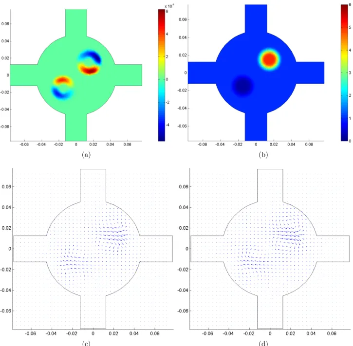
system. (b) Picture of the experiment phantom for the first ex-perimental setup explained in section 3.1.3. The balloon inside the phantom acts as an insulator and it isolates its inside solution from the background solution. (c) Illustration of the center trans-verse slice of the phantom where z = 0. The directions of two orthogonal current injection profiles are also shown. . . 22 3.2 Figures at the central slice of the simulation phantom: (a)
simu-lated ∇2B
z, (b) actual conductivity distribution, (c) quiver plot
of the actual difference current density distribution (x− and y− components), (d) quiver plot of the reconstructed J∗ . . . 26
3.3 Reconstructed conductivity in the simulations: (a) the recon-structed conductivity distribution at the center slice, (b) the re-constructed conductivity profile on the x = y line at the center slice. (a) and (b) are obtained when a single current injection is used without stabilization. (c) and (d) are same as (a) and (b) but with the SUPG stabilization applied in the solution. (e) and (f) are same as (a) and (b) but when two current injections are utilized without stabilization. . . 28
3.4 Reconstructed conductivity in the simulations when conductivity change is sharp: (a) reconstructed conductivity distribution at the center slice, (b) the reconstructed (solid line) and actual (broken line) conductivity profiles on the x = y line at the center slice. . . 29
3.5 Simulation results for the evaluation of the performance of the algorithm against noise: (a) Noisy ∇2Bz for SN R = 180 and
TC = 50ms, (b) Quiver plot of calculated J∗ using noisy ∇2Bz,
(c) reconstructed conductivity distribution at the center slice, (d) reconstructed conductivity profile on the x = y line at the center slice. (c) and (d) are obtained when no stabilization is applied. (e) and (f) are same with (c) and (d) but with SUPG stabilization applied. . . 31 3.6 Input data and the reconstructed current densities for the first
experimental setup explained in Section 3.1.3. (a) and (b) are
∇2B
z calculated from the measured Bz for two current injections
respectively, (c) and (d) are filtered versions of∇2B
z given in (a)
and (b), (e) and (f) are the quiver plots of calculated J∗ for the two current injections respectively . . . 33 3.7 Reconstructed conductivity distributions for the first experimental
setup explained in Section 3.1.3. (a) reconstructed conductivity distribution at the center slice of the phantom, (b) reconstructed conductivity profile on the x = y line at the center slice. (a) and (b) is obtained when the original∇2Bz (no filter) is used without
stabilization. (c) and (d) are same with (a) and (b) but the filtered
∇2B
z is used without stabilization. (e) and (f) are same with (a)
and (b) but the original ∇2Bz (no filter) is used with the SUPG
stabilization. (g) and (h) are same with (a) and (b) but the filtered
∇2B
3.8 Results for the second experimental setup explained in Section 3.1.3). (a) and (b) are ∇2Bz calculated from the measured Bz
for two current injections respectively. ∇2B
z is multiplied with a
cosine window in the frequency domain (kmax = 300m−1). (c) the
reconstructed conductivity distribution at the center slice when no stabilization is used (d) the reconstructed conductivity distri-bution at the center slice when SUPG stabilization is used . . . . 36
4.1 Magnitudes of inverse filters: (a) −1
2πjky 1 k2 x+ky2 (b) − 1 2πjkx 1 k2 x+k2y . 46
4.2 Simulation results for the 3D FT-MRCDI: (a) initial∇2B
z (input
to the algorithm), (b)∇2Bz reconstructed at the tenth iteration,
(c, d) quiver plot of the reconstructed J∗ at the first and tenth iterations respectively, (e, f) magnitude of the reconstructed J∗ at the first and tenth iterations respectively (The region inside the object is nulled to emphasize the decrease of the magnitude outside the object throughout the iterations). . . 50
4.3 The L2-error made in the reconstruction of J∗ and the ϕ ratio as iterations proceed for two different simulation cases. (a) and (b) are drawn for the first simulation case explained in Section 3.1.2. (c) and (d) are drawn for the simulation case in which the non-zero regions of∇2B
z is closer to the boundary. . . 51
4.4 Conductivity distribution((a)) and the quiver plot of actual dif-ference current density((b)) for the simulation case in which the non-zero regions of∇2B
4.5 Simulation results for the 3D FT-MRCDI when the non-zero re-gions of ∇2Bz is closer to the boundary : (a) initial∇2Bz (input
to the algorithm), (b)∇2B
z reconstructed at the tenth iteration,
(c, d) quiver plot of the reconstructed J∗ at the first and tenth iterations respectively, (e, f) magnitude of the reconstructed J∗ at the first and tenth iterations respectively (The region inside the object is nulled to emphasize the decrease of the magnitude outside the object throughout the iterations). . . 53 4.6 Simulation results for the 3D FT-MRCDI when noise is added
to ∇2B
z: (a) initial ∇2Bz (input to the algorithm), (b) ∇2Bz
reconstructed at the tenth iteration, (c, d) quiver plot of the re-constructed J∗ at the first and tenth iterations respectively, (e, f) magnitude of the reconstructed J∗ at the first and tenth iterations respectively (The region inside the object is nulled to emphasize the decrease of the magnitude outside the object throughout the iterations). . . 54 4.7 Experimental results for the first experimental setup: (a) initial
∇2B
z (input to the algorithm), (b) ∇2Bz at the eighth iteration,
(c, d) quiver plot of the reconstructed J∗ at the first and eighth iterations respectively, (e, f) magnitude of the reconstructed J∗ at the first and eighth iterations respectively (The region inside the object is nulled to emphasize the decrease of the magnitude outside the object throughout the iterations). . . 56
4.8 The iteration number versus the ϕ ratio: (a) the first experimental setup, (b) the second experimental setup. . . 57
4.9 Experimental results for the second experimental setup: (a) initial
∇2B
z (input to the algorithm), (b)∇2Bz at the seventh iteration,
(c, d) quiver plot of the reconstructed J∗ at the first and seventh iterations respectively, (e, f) magnitude of the reconstructed J∗ at the first and seventh iterations respectively (The region inside the object is nulled to emphasize the decrease of the magnitude outside the object throughout the iterations). . . 58
A.1 The solution of equation (A.2): (a) β = 1, k = 0 and u(0) = 0,
u(1) = 1 (b) β = 1, k = 0 and u(0) = 0, u(1) = 0 (c) β = 1, k = 1/194 and u(0) = 0, u(1) = 0 (d) β = 1, k = 10/194 and u(0) = 0, u(1) = 0 . . . . 67
B.1 Simulation results for the triangular mesh based MRCDI: (a) sim-ulated∇2Bz, (b) quiver plot of the actual difference current
den-sity distribution (x− and y− components), (c) quiver plot of the J∗ reconstructed using the method proposed by Park et al. , (d) quiver plot of the J∗reconstructed using the triangular mesh based MRCDI method. . . 73
B.2 Reconstructed conductivities using triangular mesh based MREIT in the simulations: (a) the reconstructed conductivity distribution at the center slice, (b) the reconstructed conductivity profile on the x = y line at the center slice. (c) and (d) are same as (a) and (b) but reconstructions are made with noisy ∇2Bz (SN R = 180
B.3 Simulation results for the evaluation of the performance of the triangular mesh based MRCDI against noise: (a) Noisy∇2Bz for
SN R = 180 and TC = 50ms, (b) quiver plot of J∗ reconstructed
using the method proposed by Park et al. from noisy ∇2B
z, (c)
quiver plot of the J∗reconstructed using the triangular mesh based MRCDI method from noisy∇2B
z. . . 76
B.4 Experimental results for the first experiment setup explained in Section 3.1.3: (a) and (b) are quiver plots of J∗ at the center slice reconstructed using the triangular mesh based MRCDI method from noisy∇2B
z for two current injection directions respectively,
(c) is the conductivity distribution at the center slice reconstructed using the triangular mesh based MREIT. . . 78
B.5 Experimental results for the second experiment setup explained in Section 3.1.3: (a) and (b) are quiver plots of J∗ at the center slice reconstructed using the triangular mesh based MRCDI method from noisy∇2Bz for two current injection directions respectively,
(c) is the conductivity distribution at the center slice reconstructed using the triangular mesh based MREIT. . . 79
List of Tables
1.1 Typical electrical conductivities of some biological tissues at low frequencies (reproduced from [4]) . . . 2
Chapter 1
INTRODUCTION
1.1
Motivation
In Magnetic Resonance Electrical Impedance Tomography (MREIT), electrical current is injected into a conductive object such as the human-body via sur-face electrodes. The resulting internal current generates a magnetic flux density distribution both inside and outside the object. The magnetic flux density in-side the object is measured using a Magnetic Resonance Imaging (MRI) system, and from this measured magnetic flux density distribution, the internal electrical conductivity distribution of the object is reconstructed.
Imaging electrical conductivity distribution of biological tissues has been an active research area in the field of medical imaging for decades. Electrical con-ductivity greatly varies in different tissues of human body since each tissue has different cell concentration, cellular structure, membrane capacitance, and so on [1]-[3]. Electrical conductivity of human tissues is also a function of the frequency of the applied current. In MREIT and MRCDI, very low frequencies are consid-ered (less than 1 kHz) and therefore effects of permittivity is ignored and only
conductivity is considered. Typical electrical conductivities of different biological tissues at low frequencies are given Table 1.1 [4].
The conductivity distribution provides both an anatomical image and a dif-ferent contrast mechanism. More importantly, the electrical conductivity also depends on the pathological state of the tissues which means the electrical con-ductivity imaging can be used for detection and characterization of, for instance, tumors [5]-[7].
Similar to MREIT, in Magnetic Resonance Current Density Imaging (MR-CDI), the magnetic flux density due to injected currents is measured via an MRI system. The internal current density distribution is then reconstructed using this data. MRCDI is strictly related to MREIT in the sense that some MREIT algorithms require the current density distribution to be known and in other algorithms the current density may be calculated once the conductivity is ob-tained. Besides being a companion problem to MREIT, MRCDI itself has also potential medical applications [8]-[15]. There are many therapeutic techniques in which currents are injected to the body (e.g. cardiac defibrillation and pac-ing, electrocautery, and some treatment methods in physiotherapy). Knowledge of current density distribution would be useful in planning and designing such therapeutic techniques.
Table 1.1: Typical electrical conductivities of some biological tissues at low fre-quencies (reproduced from [4])
Tissue Frequency (kHz) Conductivity (S/m) Cerebrospinal fluid (human) 1 1.56
Blood (human) DC 0.67
Plasma (human) DC 1.42
Skeletal muscle (longitudinal fibers) (human) DC 0.41 Skeletal muscle (transverse fibers) (human) 0.1 0.15
Fat (dog) 0.01 0.04
1.2
MRCDI and MREIT Problem Definitions
1.2.1
Forward Problem
Let Ω be a connected and bounded domain in R3 representing the internal re-gion of a three-dimensional electrically conducting object in which the electrical current density and the conductivity distribution is to be imaged. DC current of magnitude I is applied between two electrodes attached on the boundary of the domain which is denoted by ∂Ω. The electric potential, ϕ(x, y, z), dictated by the current injection satisfies the boundary-value problem with Neumann boundary condition which is given as
∇ · σ∇ϕ(x, y, z) = 0 in Ω σ∂ϕ∂n = g on ∂Ω
(1.1)
where σ is the electrical conductivity, n is the unit outward normal along the boundary ∂Ω, ∫
E±
g ds = ±I on electrodes (E± denotes one of the electrodes on
∂Ω and sign depends on whether current is injected through or sunk from the
electrode considered), and g = 0 on ∂Ω other than electrodes. The current density, J, is given by J = σE where E = −∇ϕ is the electric field. Once the problem given by Equation 1.1 is solved for electric potential, it easy to calculate the current density distribution.
In MREIT and MRCDI, currents of very low frequency are injected into the imaging object and therefore static version of Maxwell’s equations are used. In the static assumption, the displacement current, ∂D∂t, and the magnetic induction,
∂B
∂t, are negligible. Therefore J = ∇ × B/µ0 and ∇ × E = 0.
The magnetic flux density generated by the current density distribution in Ω is given by Biot-Savart law as
B(r) = µ 4π ∫ Ω J(r)× r− r ′ |r − r′|3 dr ′ (1.2)
where B(r) is the generated magnetic flux density, r is the position vector inR3,
and µ is the magnetic permeability which can be assumed to be space-invariant and has the free space value of µ0 = 4π× 10−7 H/m for body tissues.
Given the conductivity distribution in Ω, the object and boundary geometry, and the electrode configuration, the forward problem of MRCDI and MREIT is the calculation of the magnetic flux density which is generated by the internal current density. The internal current density distribution is calculated from the electric potential which is the solution of Equation 1.1. The solution of forward problem is necessary for the generation simulated data which are used to test the developed algorithms. Furthermore, as will be discussed in Section 1.3, some MRCDI and MREIT algorithms, including the MREIT algorithm proposed in this thesis, requires the solution of the current density distribution when homo-geneous conductivity is assumed in Ω.
1.2.2
Inverse Problem
The inverse problem of MRCDI is the reconstruction of the current density from the measured magnetic flux density. Some early MRCDI algorithms assume that all components of the magnetic flux density are measured. However, as will be discussed in Section 1.3, measurement of all components of the magnetic flux density is impractical, and therefore currently most MRCDI algorithms utilize only one component of the magnetic flux density, namely Bz, if main magnetic
field of the MRI scanner is assumed to be the z- direction. Bz is generated only
by transverse (x- and y- components) current density and the relation given in Equation 1.2 is written only for Bz as
Bz(x, y, z) = µ0 4π ∫ Ω (y− y′)Jx(x′, y′, z′)− (x − x′)Jy(x′, y′, z′) [(x− x′)2+ (y− y′)2+ (z− z′)2](3/2) dx ′dy′dz′. (1.3)
On the other hand, the inverse problem of MREIT is the reconstruction of the conductivity distribution from the measured magnetic flux density. Some early MREIT algorithms assume that that all components of the magnetic flux density are measured and all components of the current density are calculated from Ampere’s Law (J = ∇ × B/µ0) so that the inverse problem of MREIT
reduces to reconstruction of the conductivity from the current density. These algorithms often called J-based MREIT algorithms. Recently most algorithms utilize only Bz, which are often called Bz-based MREIT algorithms.
Although some Bz-based MREIT problems directly utilize Bz data, other
algorithms use the Laplacian of Bz (∇2Bz). Taking the curl of both sides of
Ampere’s Law (J = ∇ × B/µ0), and using the vector identity ∇ × ∇ × B =
∇(∇ · B) − ∇2B together with the fact that∇ · B = 0, the following expression,
which relates the x- and y- components of the current density distribution to
∇2B z, is obtained [8]: ∂Jx ∂y − ∂Jy ∂x = ∇2B z µ0 (1.4) Since current density is given by J = σE and ∇ × E = 0, we also have
1 σ(Jx ∂σ ∂y − Jy ∂σ ∂x) = ∇2B z µ0 (1.5) For the∇2Bz-based MREIT algorithms, the inverse problem is the reconstruction
of the conductivity using the relation given in Equation 1.5.
1.3
Review of Previous Studies in MRCDI and
MREIT
MRCDI was introduced in 1989 by Joy et al. [16]. In their study, by physically rotating the experiment phantom inside the MRI scanner, they measured all components of the magnetic flux density generated by the injected current. Since only the component of the magnetic flux density parallel to the direction of the
main magnetic field of the MRI scanner can be measured at one time, object rotations are necessary for measuring all components of the magnetic flux density. The current density distribution was calculated from Ampere’s Law (J = ∇ × B/µ0). As an experiment phantom, they prepared two isolated cylindrical tubes
one within the other and both tubes were filled with electrolyte. The current was applied between two ends of the inner tube and a uniform current flowing only in one direction was obtained. Later in 1991, Scott et al. used a similar procedure to reconstruct nonuniform current density flowing in all directions [8]. One year later, Scott et al. published their study in which they investigated the sensitivity of MRCDI to both random noise and systematic errors [17]. There are some other investigators who have also measured all components of the magnetic flux density and utilized Ampere’s Law to reconstruct the current density. In 1998, Ey¨ubo˘glu et al. [18] reported that they have reconstructed current density magnitude of which is lower than the current density reconstructed by Scott et
al. . Also they reconstructed the current density in a slice more close to the
electrodes. They used a similar experimental phantom that was used by Scott et
al. in 1991. Other studies may be listed as applications of the MRCDI procedure
proposed by Joy et al. [8]-[15].
In practice, rotating the object inside an MRI scanner is not desirable be-cause of possible misalignments after the rotation. Furthermore, for long objects, subject rotations are in fact impossible in a conventional closed bore MRI sys-tem. Last not least, since the experiment must be repeated three-times in order to measure all three components of the magnetic flux density, total scan time becomes three times higher. Therefore most MRCDI and MREIT algorithms use only one component of the measured magnetic flux density, namely Bz, where
z- direction is the direction of the main magnetic field of the MRI scanner. It
was shown by Park et al. that the transverse current density distribution cannot be fully recovered using only Bz information unless the difference between the
homogeneous conductivity is negligible [19] . Nevertheless, in their study, Park
et al. have also developed an algorithm by which Jx and Jy distributions can be
estimated for a certain slice given the∇2B
z data for that slice. They have called
this estimated transverse current density the “projected current density” which is the recoverable portion of the actual current density.
Besides spatial domain MRCDI algorithms, some frequency domain tech-niques for MRCDI is also suggested [20]-[22]. ˙Ider et al. have developed Fourier Transform (FT)-based MRCDI algorithms utilizing only Bz for two- and
three-dimensional problems [22]. For two-dimensional problems where the current density has no z- component, the proposed algorithm iteratively reconstructs both the current density on an xy- plane inside the object and also the magnetic flux density on the same xy- plane outside the object. For three-dimensional problems, another algorithm has been developed in the same study by which the “projected current density” at any desired slice is iteratively reconstructed from the ∇2B
z data for that slice. The algorithm for three-dimensional case
is named “3D Fourier Transform-Magnetic Resonance Current Density Imaging (FT-MRCDI)” and the work done for this thesis also includes the algorithm developed for 3D FT-MRCDI which is discussed in Chapter 4.
As indicated in Section 1.1, MRCDI and MREIT are companion problems such that in many MREIT algorithms current density is also reconstructed. In the following, some MREIT algorithms will be discussed in which the current density is reconstructed as a part of the algorithm or may be reconstructed as an additional information once the conductivity is reconstructed. The MREIT algorithms fall into two categories which are J-based and Bz-based algorithms
respectively. While early MREIT algorithms are members of the first group, recently most MREIT algorithms are members of the latter group.
In J-based MREIT algorithms, all components of the magnetic flux density is measured from which J is calculated using Ampere’s Law. These algorithms con-centrate on reconstructing the conductivity distribution from the reconstructed current density. In 1992, Zhang proposed the first J-based MREIT algorithm in his MSc thesis and so the MREIT concept was first introduced [23]. Apart from this study, the MREIT concept is also introduced by Woo et al. [24] in 1994, and by Birgul and ˙Ider [25] in 1995 independently. These two studies also involve J-based algorithms. Other J-based algorithms are given in [26]-[31].
On the other hand, Bz-based MREIT algorithms provide us with the ability
to reconstruct the conductivity distribution using only Bz which is
advanta-geous over J-based algorithms since impractical object rotations are not needed. Therefore, today, most MREIT algorithms fall into category of Bz-based MREIT
algorithms.
In 1995, Birgul and ˙Ider proposed the first Bz-based algorithm [25]. They
formed a sensitivity matrix in order to linearize the relation between the con-ductivity and Bz which is given by Equations 1.1 and 1.3 considering the fact
that J =−σ∇ϕ. The obtained sensitivity matrix is inverted using truncated sin-gular value decomposition. They have published simulation results [32] and the experimental results are given in [33] for the proposed sensitivity matrix based MREIT algorithm.
As mentioned in Section 1.2.2, some Bz-based MREIT algorithms utilize the
Laplacian of Bz (∇2Bz) in which∇2Bz is calculated from the measured Bz before
the reconstruction algorithm starts. The relation between the conductivity (σ), current density (J) and the Laplacian of Bz (∇2Bz) was given in Equation 1.5.
If Jx and Jy are known for a certain slice (intersection of the object with a
certain z = constant plane) then the transverse gradient of the conductivity, (∂σ∂x, ∂σ∂y), can be calculated from the ∇2B
z data obtained for that slice only.
of conductivity at a certain slice is possible so that measuring Bz in the whole
domain is not necessary. If the electric potential (ϕ) is used, Equation 1.5 may be written as ∂σ ∂x ∂ϕ ∂y − ∂σ ∂y ∂ϕ ∂x = ∇2B z µ0 . (1.6)
In 2003, Seo et al. proposed a∇2Bz-based iterative algorithm which depends on
the solution of the above equation [34]. For the first iteration, they assumed a homogeneous conductivity and solved the forward problem to find electric poten-tial and they used this electric potenpoten-tial to solve Equation 1.6 for the gradient of the conductivity in each MR pixel. They used two orthogonal current injections to obtain a unique solution. For the calculation of the conductivity from its gra-dient, they utilized a line integral method. The newly calculated conductivity is used for the next iteration and the iterations stop if the change in the con-ductivity for the consecutive iterations is sufficiently small. Oh et al. used the same algorithm with the difference that they utilized a layer potential technique to calculate the conductivity distribution from its gradient [35]. They called this algorithm as “Harmonic Bz algorithm”.
In 2004, ˙Ider and Onart modified Equation 1.5 to obtain
∇2B z = µ0(Jx ∂R ∂y − Jy ∂R ∂x) (1.7)
where R = ln σ [36]. They proposed an iterative algorithm based on the above equation. For the first iteration, they assumed a homogeneous conductivity and solved for the current density. Next, they used the finite difference approximation to obtain a matrix system for the solution of R. Upon the solution of the matrix system, R is obtained directly in each pixel. They used this R in the next iteration and the iterations stop if the change in R for the consecutive iterations are sufficiently small.
In 2008, Nam et al. used the “projected current density” [19] in Equation 1.7 to find the transverse gradient of R in each pixel at the slice of interest [37]. Starting from the gradient distribution, they utilized a layer potential technique,
suggested by Oh et al. [35], to reconstruct the conductivity distribution on that slice.
1.4
Objective and Scope of the Thesis
This thesis covers the research regarding both the hardware and the algorithm de-velopment aspects of MREIT and MRCDI. As mentioned previously, for MREIT and MRCDI, currents are injected through surface electrodes into the imaging object which requires an MRI compatible constant current source. Therefore, on the hardware side, a current source which is used for injecting currents in the experiments is designed and developed.
On the other hand, we have developed two new reconstruction algorithms one for MREIT and one for MRCDI. For MREIT, the devoloped algorithm is named
MREIT based on the solution of the convection equation. In this algorithm,
the relation which is given in Equation 1.7 is put into the form of the steady-state scalar convection equation. Convection equation is a special case of the more general convection-diffusion equation and describes the distribution of a physical quantity (e.g. concentration, temperature) under the effect of two basic mechanisms, convection and diffusion. The convection-diffusion equation arises in many physical phenomena such as distribution of heat, fluid dynamics etc. Although physically no convection mechanism exists in the MREIT problem, it can nevertheless be handled as a convection problem solely from a mathematical point of view. Furthermore, because the convection equation by itself does not always yield stable numerical solutions, introduction of a diffusion term as a stabilization technique is customary. Therefore, in MREIT based on the solution
of the convection equation, the MREIT problem is handled as a
convection-diffusion problem and the advanced numerical methods developed for the solution of the convection-diffusion equation by using finite element method (FEM) are
adapted and used for solving the MREIT problem. The methods are then tested both with simulated and experimental data.
For MRCDI, a spatial frequency domain based MRCDI algorithm which is named Three-dimensional Fourier transform MRCDI, is developed. In this al-gorithm, in a imaging slice, Equation 1.4 and divergence-free condition of the current density is utilized together in the frequency domain. To our knowledge, the proposed algorithm is the only frequency domain MRCDI algorithm for 3D problems. The results obtained from both the simulated data and the experi-mental data are presented.
Noise is inherent in the actual Bz measurements. Therefore it is important to
evaluate the performance of any reconstruction algorithm for MREIT or MRCDI. In this thesis, we also provide simulation results for both developed MREIT and MRCDI algorithms when random noise is added to the simulated∇2Bz.
1.5
Organization of the Thesis
This thesis consists of five chapters. Chapter 2 discusses the designed data col-lection system for MREIT and MRCDI. In this chapter, the MRI pulse sequence, which is used for measuring magnetic flux density due to the injected currents is discussed. Also the designed current source is described. Chapter 3 and 4 discusses the developed MREIT based on the solution of the convection equation algorithm and Three-dimensional Fourier transform MRCDI algorithms respec-tively. The simulation and experimental methods and the results obtained using these methods are given in each chapter in order to evaluate the performance of the proposed algorithms. Finally, Chapter 5 provides conclusions to the thesis.
Chapter 2
DATA COLLECTION SYSTEM
FOR MREIT AND MRCDI
In MRCDI and MREIT, an MRI scanner is used to measure the magnetic flux density distribution due to the injected currents. It is known that an MRI system is only sensitive to the transverse magnetization and only z- component of the generated magnetic flux density can effect transverse magnetization by providing additional phase to the spins (z- direction is the direction of the main magnetic field of the MRI scanner). Therefore only z- component of the generated magnetic flux density, namely Bz, can be measured at one time, and we will
discuss measurement of only Bz in this chapter. It is important to remind that,
in order to measure other components of the generated magnetic flux density, the imaging object could be rotated inside the MRI scanner. However, in practice, object rotations are impractical as discussed in Chapter 1.
2.1
Measurement of B
zvia an MRI Scanner
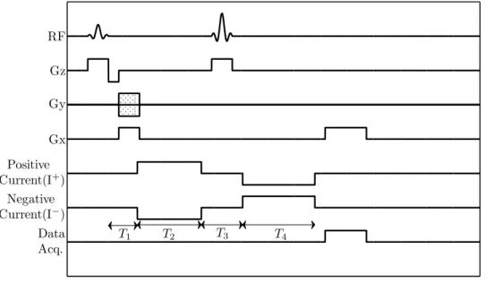
In order to measure Bz via an MRI scanner, several MRI pulse sequences is
proposed [16], [38]-[43]. In this study, the conventional spin-echo MREIT pulse sequence proposed by Joy et al. [16] is used. The timing diagram of the sequence is given in Figure 2.1. As evident from Figure 2.1, the imaging slice is transversal and so Bz is measured in a transversal slice, although sagittal and coronal slices
are possible. Two acquisitions are required in which positive and negative current injections are used separately. The complex k-space data obtained using this pulse sequence can be written for positive and negative current injections as
S±(m, n) = ∫ R2
M (x, y) exp (jδ(x, y)) exp (±jγBz(x, y)Tc)
exp (−j2π(m∆kxx + n∆kyy))dxdy
(2.1)
where M (x, y) is the transverse magnetization which is a function of spin density and T1, T2 decay constants, δ(x, y) is the systematic phase artifact in radians, γ
is the gyromagnetic ratio (26.7519× 10⁷ rad/T s), B
z is the z- component of the
magnetic flux density due to the injected current, Tcis the total current injection
time and kx, ky are the spatial frequency components in x- and y- directions.
Two complex images for positive and negative current injections, which can be obtained fromS±(m, n) using two-dimensional discrete inverse Fourier transform (DFT), are given as
M±(x, y) = M (x, y) exp (jδ(x, y)) exp (±jγB
z(x, y)Tc). (2.2)
The phases of two images in radians are
Φ1 = δ(x, y) + γBz(x, y)Tc and Φ2 = δ(x, y)− γBz(x, y)Tc. (2.3)
from which Bz can be calculated by subtracting phases to eliminate δ(x, y) and
dividing by two (Bz(x, y) = (Φ1 − Φ2)/(2γTc)). Note that the obtained phase
images are most likely wrapped and in order to unwrap the phase images, Gold-stein’s phase unwrapping algorithm is used in this study [44].
Data Acq. Negative Current(I−) Positive Current(I+) Gx Gy Gz RF T1 T2 T3 T4
Figure 2.1: The conventional MREIT pulse sequence used in the study.
2.2
MR Compatible Current Source for
MR-CDI and MREIT
In MRCDI and MREIT modalities, an MRI compatible constant current source is required to inject currents into the subject through surface electrodes. The required current waveform is given in Figure 2.1. The current injection cycle starts T1 milliseconds after the 90◦ RF excitation pulse. Therefore the current
source must be triggered by the MRI system to indicate the location of the excitation RF pulse in time. Once triggered by the MRI system, the current source must apply currents with respect to T1, T2, T3 and T4 as shown in Figure
2.1. Since TEcan be differently selected for each experiment, T1-T4is not constant
and the current source must be designed such that these values is entered for each experiment.
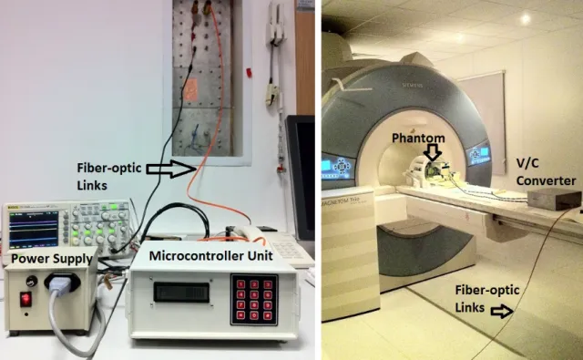
In this study, a current source system which has above specifications is de-signed and implemented for the MRCDI and MREIT experiments. The dede-signed
system has three parts (each part placed in a different box), namely power supply, microcontroller, and voltage-to-current converter (Figure 2.2).
Figure 2.2: Hardware Setup: On the left, microcontroller and power supply units which are located near MRI console are shown. The fiber-optic links which carry A and B signals from the microcontroller unit to the voltage-to-current (V/C) converter are also shown. On the right, the V/C converter which are located in the scanner room is shown with the MRI scanner.
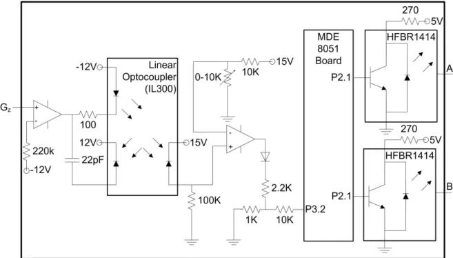
The circuit diagram for the microcontroller part is given in Figure 2.3. The microcontroller part mainly produces A and B signals (Figure 2.4) which are then sent to the current source box via fiber-optic links. The required trigger is taken from the negative edge at the onset of the refocusing pulse of the z-gradient, which is the only negative part in the z-gradient signal as shown in Figure 2.1. The z-gradient signal is isolated from the microcontroller box circuit by using a linear optocoupler such that the gradient signal on the isolated side is transferred to the non-isolated side with a DC offset. The isolated side of the circuit operates at ±12 V obtained from lead-acid batteries whereas the non-isolated part operates at ±15 V and 8 V obtained from the power supply part. Once the signal is transferred to the non-isolated part, the signal is entered to a
Figure 2.3: Curcuit diagram for microcontroller part. Gz stands for z-gradient
signal. HFBR1414 is a optical transmitter which converts electrical signals to optical signals
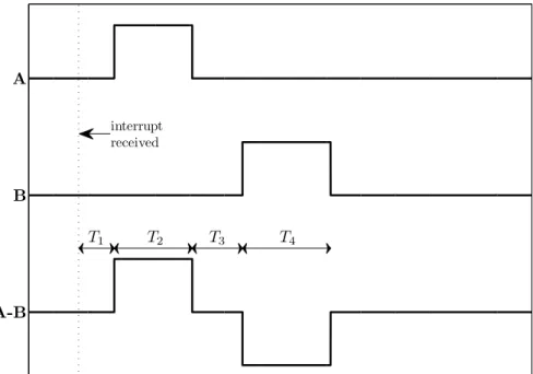
comparator such that another signal, which becomes 15 V during the refocusing part of the gradient signal and stays at−15 V otherwise, is produced. This signal is input to the interrupt port of the microcontroller board after eliminating the negative part with a diode and the signal level is decreased by a voltage-divider circuit. The microcontroller board consists of a 8051 microcontroller and driving circuitry. The board is programmed to produce A and B signals with respect to the T1-T4 which are entered with the help of a numpad and an LCD. A and B
signals are sent to the voltage-to-current converter part by using digital optical transmitters (Avago Technologies, HFBR 1414). The circuit diagram for the voltage-to-current converter part is given in Figure 2.5 where RL represents the
phantom. The voltage-to-current converter part converts optical A and B signals into the electrical signals and then subtracts B from A to obtain the desired current injection waveform as a voltage as shown in Figure 2.4. This voltage waveform is then converted to the current waveform via a simple opamp circuit. The magnitude of the current may be adjusted with the resistor at the negative
A-B B A T1 T2 T3 T4 interrupt received
Figure 2.4: A and B signals
input of the opamp. The voltage-to-current converter part operates at ±12 V obtained from the lead-acid batteries. The voltage-to-current converter part is the only part of the current source system which is placed inside the scanner room in the experiments (Figure 2.2). Therefore the circuit and the batteries are placed in an aluminum case. For the output cables which transfer current from voltage-to-current converter part to the phantom (the imaging object), feed-through filters are used. Furthermore, fiber-optic links are used between microcontroller part and the voltage-to-current converter part in order to preclude any possible noise from microcontroller box inside the scanner room.
Figure 2.5: Circuit diagram for voltage-to-current converter part. RL denotes
the load resistor which is the experimental phantom in our case. HFBR2412 is a optical receiver which converts optical signals to electrical signals
Chapter 3
MREIT BASED ON THE
SOLUTION OF THE
CONVECTION EQUATION
3.1
Methods
3.1.1
The Algorithm
The relation between electrical conductivity (σ), current density (J), and Lapla-cian of the Bz (∇2Bz) was derived in Section 1.2.2 as
1 σ(Jx ∂σ ∂y − Jy ∂σ ∂x) = ∇2B z µ0 . (3.1)
Defining R = ln σ, Equation 3.1 can be expressed as [36]
∇2B z = µ0(Jx ∂R ∂y − Jy ∂R ∂x). (3.2)
Furthermore defining eJ = (−Jy, Jx), and ∇R = (∂R∂x,∂R∂y), Equation 3.2 can be
discussed in the Appendix A, as
eJ · ∇R = ∇2Bz
µ0
. (3.3)
In this equation, eJ may be recognized as the convective field defined in Equation A.1, R is the scalar field to be solved and ∇2Bz
µ0 is the source term.
Apart from R, the eJ vector is also unknown in Equation (3.3) since the current density is not known. The actual current density consists of two components, namely J0 and Jd, where J0 is the current density distribution obtained by
solving the forward problem for the homogenous conductivity distribution and Jd is defined as the difference current density such that Jd= J− J0. Since only
Bz is utilized, only an estimate for the actual difference current density, namely
J∗, can be calculated [19]. J∗ is calculated from the relation J∗ = (∂β∂y,−∂β∂x) where β is the solution of the two-dimensional (2-D) Laplace equation given as
∇2β = ∇2Bz
µ0
in Ω′ and β = 0 on ∂Ω′ (3.4)
where Ω′ is the intersection of Ω with a z = constant plane (the slice of interest) and ∂Ω′ is the boundary of the intersection. Once J∗ is obtained, the projected current density which is defined as JP = J∗+ J0 is calculated. eJ = (−JyP, JxP) is then substituted into Equation (3.3) so that it can be solved for R.
For the numerical solution of Equation (3.3) on the slice of interest, fi-nite element method (FEM) is used. In the FEM formulation, either standard Galerkin weighted residual method [45], or Galerkin weighted residual method with streamline upwind Petrov-Galerkin (SUPG) stabilization [46], which is dis-cussed in detail in Appendix A, is used.
In general more than one current injections may be used for MREIT. If two orthogonal current injections are used, the final matrix system for Equation (3.3)
is written as K1 K2 RN×1 = b1 b2 (3.5)
where N is the number of nodes in the triangular mesh at the slice of interest, and K1, K2 and b1, b2 are obtained for two orthogonal current injections by
using Galerkin weighted residual FEM with or without SUPG stabilization. In solving Equation (3.3) boundary conditions must also be considered. When Dirichlet boundary conditions are used, some nodes on the boundary are assigned conductivity values and the matrix system given in (3.5) is reduced. The reduced system is solved using singular value decomposition (SVD) without truncation. If only one current injection is used, the matrix system involving only K1 and
b1 is solved.
3.1.2
Simulation methods
For simulations, a cylindrical phantom of height 20 cm and diameter 9.4 cm is modeled (Figure 3.1(a)) using Comsol Multiphysics software package in order to solve for electric potential in the three-dimensional forward problem explained in Section 1.2.1. The regions that the current is injected and sunk are 3 cm re-cessed from the body of the phantom to model the phantom used in experiments. Current is injected through circular electrodes of diameter 1 cm located at the ends of recessed parts. Cross-section of the recessed parts is square with edges of 2.5 cm long. Current is applied between opposite electrodes and two orthogonal current injection directions are possible as shown in Figure 3.1(c). The amount of injected current is 10 mA and total current injection time is 50 ms.
Background conductivity of the simulation phantom is taken to be 1 S/m and two cylindrical regions of conductivity anomaly are modeled inside the phantom. Figure 3.2(b) shows the conductivity distribution of the simulation phantom for the z = 0 slice. The conductivities of the low and high conductivity anomalies are 0.2 S/m and 5 S/m respectively. However the change of conductivity from the background value to the low and high values in the anomalous regions is not sharp but it is tapered as shown Figure 3.3(b), (d) and (f). Tetrahedral
(a) (b)
(c)
Figure 3.1: (a) Phantom model drawn using Comsol Multiphysics. Two cylindri-cal regions which have different conductivity than the background are also seen. The height of the first cylindrical region is 10 cm while the height of the other cylindrical region is 8 cm. z-direction is the direction of the main magnetic field of the MRI system. (b) Picture of the experiment phantom for the first exper-imental setup explained in section 3.1.3. The balloon inside the phantom acts as an insulator and it isolates its inside solution from the background solution. (c) Illustration of the center transverse slice of the phantom where z = 0. The directions of two orthogonal current injection profiles are also shown.
elements with quadratic shape functions are used for the FEM formulation of the three-dimensional problem. There are 1,159,225 tetrahedral elements and 212,007 nodes (1,608,578 degrees of freedom since quadratic shape functions are used) in total. Once the forward problem is solved, the current density distribu-tion is obtained on the nodes of a 2-D triangular mesh representing the plane at
z = 0. The relation given in (1.4) is then used to calculate the simulated ∇2B
z.
There are 5088 triangles and 2657 nodes in the 2-D triangular mesh.
The simulated∇2Bzat the slice of interest is the input data for reconstructing
the projected transverse current density on that slice. Conductivity distribution is then reconstructed by solving Equation (3.3) using the proposed method. Er-rors made in the reconstructed projected current density and the reconstructed conductivity in the slice of interest are calculated using the relative L2-error
formula: EL2(JP) = 100 [∑M i=1((Jxia−JxiP) 2 +(Ja yi−JyiP) 2 ) ∑M i=1(Jxia2+Jyia2) ]1/2 EL2(σ) = 100 [∑N j=1(σja−σj)2 ∑N j=1σaj 2 ]1/2 (3.6) where Ja xi and J a
yi are the x- and y- components of the actual current density
at the center of the i’th triangle, JP
xi and J
P
yi are the x- and y- components
of the reconstructed projected current density, σja and σj are the actual and
reconstructed conductivity distributions at the j’th node respectively, N is the number of nodes in the 2-D mesh and M is the number of the triangles in the 2-D mesh.
3.1.3
Experimental methods
Two different experimental setups are prepared for the experiments. For the first experimental setup, an experimental phantom, dimensions of which are the same as the simulation phantom explained in section 3.1.2, is manufactured. The
phantom is first filled with the background solution (12 gr/l NaCl and 1.5 gr/l CuSO4.5H2O). An insulator object is then obtained by filling a cylindrically
shaped balloon with the background solution so that the solutions inside and outside the balloon have no contact (Figure 3.1(b)). Current is injected through electrodes facing each other and data is obtained for two orthogonal current injection profiles. Bz is measured at three consecutive (no gap) transverse slices
of thickness 5 mm. ∇2B
z is calculated at the middle slice which is centered to
z = 0 plane of the phantom. For the Laplacian operator the finite difference
approximation is utilized: ∇2B z c(m, n) = Bz c(m+1,n)−2B(∆x)z c(m,n)+B2 z c(m−1,n) + Bz c(m,n+1)−2Bz c(m,n)+Bz c(m,n−1) (∆y)2 + Bz u(m,n+1)−2Bz c(m,n)+Bz l(m,n−1) (∆z)2 (3.7) where m = 1, ..., N , n = 1, ..., N , Bz u, Bz c, Bz l are Bz matrices obtained at the
upper, center and lower slices respectively, ∆x and ∆y are the sizes of an MR image pixel in x- and y-directions respectively, ∆z is the slice thickness and N is the size of the MR image matrix in both directions. The standard spin-echo MREIT pulse sequence, which is discussed in Section 2.1, is used. The magnitude of the applied current is 10 mA and total duration of current injection is 42 ms. The number of averages is 5, echo time (TE) is 60 ms, repetition time (TR) is
900 ms, image matrix is 128× 128 and the field of view is 180 × 180 mm. The experiments are conducted using a 3T MRI scanner (Siemens Magnetom Trio).
For the second experimental setup, the same experimental phantom is used. The phantom is filled with background solution (3 gr/l NaCl, 1 gr/l CuSO4.5H2O)
and two conductive cylindrical agar (15 gr/l agar) objects of height 7 cm and diameter 3.4 cm is placed inside the phantom. While the first object has lower conductivity (0.8 gr/l NaCl 1 gr/l CuSO4.5H2O) than the background solution
All other experiment parameters including MR imaging parameters and current injection time is the same with the first experimental setup.
3.2
Results
3.2.1
Simulation Results
Simulated∇2B
z data, actual conductivity distribution, actual difference current
density distribution (x− and y− components), and J∗ reconstructed using the method explained in Section 3.1.1 are shown in Figure 3.2 for the simulation phantom. All images are drawn for the central transverse slice of the simulation phantom where z = 0 (named as imaging slice hereafter) and when current is injected in I1 direction shown in Figure 3.1(c). The relative L2-error made in the
reconstructed J∗ is 23.59%.
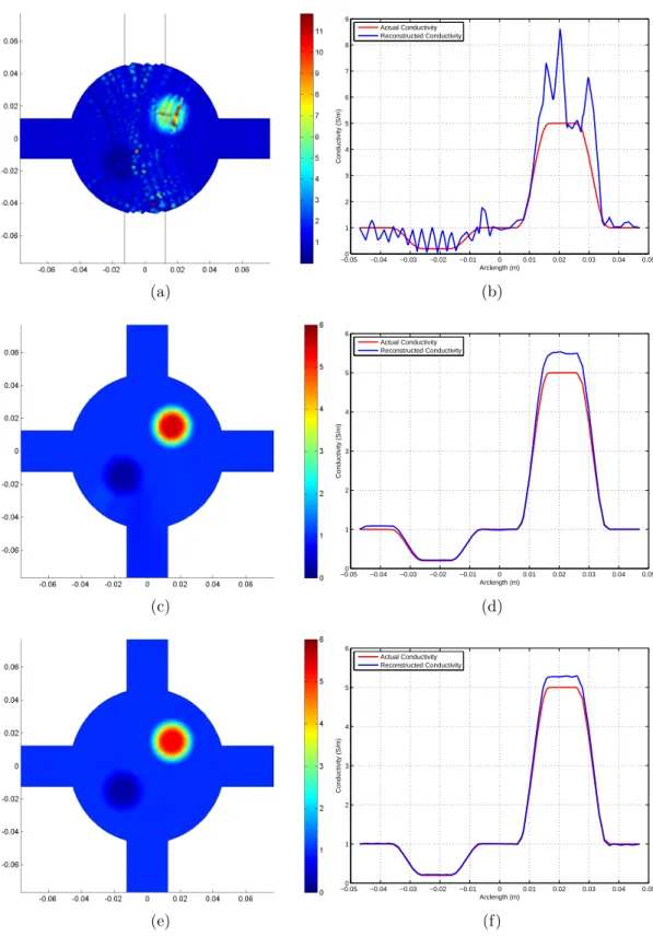
Figure 3.3(a) shows the reconstructed conductivity distribution at the imag-ing slice for the case of simag-ingle current injection (I1 direction in Figure 3.1(c)) when
no stabilization is used in the FEM with Galerkin weighted residual method. Conductivity values on the boundary are assumed to be 1 S/m (R = 0 since
R = ln σ). Reconstructed conductivity of the upper and lower recessed regions
is not shown in the figure because in these regions excessively noisy distributions of conductivity with very large variance are obtained. This is most likely due to the fact that in the upper and lower recessed regions current density is very low and therefore the convection equation is ill-defined in these regions. Next, SUPG stabilization is utilized in the numerical solution of equation (3.3) for the case of single current injection and the reconstructed conductivity distribution at the imaging slice is given in Figure 3.3(c). A more stable solution is obtained and the relative L2-error made in the reconstructed conductivity is 6.26% (L2-error in the previous case without using stabilization was 56% even excluding upper
(a) (b)
(c) (d)
Figure 3.2: Figures at the central slice of the simulation phantom: (a) simulated
∇2B
z, (b) actual conductivity distribution, (c) quiver plot of the actual difference
current density distribution (x− and y− components), (d) quiver plot of the reconstructed J∗
and lower recessed regions). Figure 3.3(b) and (d) show the reconstructed con-ductivity profiles on the x = y line of the imaging slice for the cases of without and with stabilization respectively. It is observed that oscillations seen in the profile when no stabilization is used disappear with the use of stabilization and yet transition regions of conductivity change are still well represented.
Figure 3.3(e) and (f) show the reconstructed conductivity at the imaging slice for the case of two current injections when no stabilization is used. The solution is stable even though no stabilization is utilized and the L2-error made in the reconstructed conductivity is 3.68%. With two current injections, we know that the current distribution in the recessed regions has large values at least for one of the current injection cases. Therefore, when two current injections are used, the ill-defined convection equation situation is not observed. Furthermore, when SUPG stabilization is used, no significant improvement is obtained in the recon-structed conductivity distribution. It is also important to note that, in the ex-ample investigated, the conductivity distribution does not have sharp variations nor the given boundary conditions are inconsistent, and therefore stabilization is not necessary.
The algorithm is also tested when the conductivity distribution at the imaging slice has sharp variations. For this purpose, the phantom geometry same with the previous case is used with a narrower conductivity transition region. The actual conductivity profile on the x = y line at the imaging slice is given in Figure 3.4(b) and (d). Reconstruction results for the case of two current injections are also shown in Figure 3.4. Figure 3.4(a) and (b) show the conductivity reconstructions when no stabilization is utilized. L2-error made in the reconstructed conductivity
is 15.88% and considerable oscillations are observed. However, when SUPG stabilization is used L2-error decrease to 7.11% and oscillations disappear as shown in Figure 3.4(c) and (d). Therefore, although stabilization is not found to be necessary when conductivity variations are not sharp, it is found that
(a) −0.050 −0.04 −0.03 −0.02 −0.01 0 0.01 0.02 0.03 0.04 0.05 1 2 3 4 5 6 7 8 9 Arclength (m) Conductivity (S/m) Actual Conductivity Reconstructed Conductivity (b) (c) −0.050 −0.04 −0.03 −0.02 −0.01 0 0.01 0.02 0.03 0.04 0.05 1 2 3 4 5 6 Arclength (m) Conductivity (S/m) Actual Conductivity Reconstructed Conductivity (d) (e) −0.050 −0.04 −0.03 −0.02 −0.01 0 0.01 0.02 0.03 0.04 0.05 1 2 3 4 5 6 Arclength (m) Conductivity (S/m) Actual Conductivity Reconstructed Conductivity (f)
Figure 3.3: Reconstructed conductivity in the simulations: (a) the reconstructed conductivity distribution at the center slice, (b) the reconstructed conductivity profile on the x = y line at the center slice. (a) and (b) are obtained when a single current injection is used without stabilization. (c) and (d) are same as (a) and (b) but with the SUPG stabilization applied in the solution. (e) and (f) are same as (a) and (b) but when two current injections are utilized without stabilization.
for subjects in which conductivity variations are sharp and abrupt, stabilization becomes necessary. (a) −0.050 0 0.05 0.5 1 1.5 2 2.5 3 3.5 4 4.5 5 Arclength (m) Conductivity (S/m) Actual Conductivity Reconstructed Conductivity (b) (c) −0.050 0 0.05 0.5 1 1.5 2 2.5 3 3.5 4 4.5 5 Arclength (m) Conductivity (S/m) Actual Conductivity Reconstructed Conductivity (d)
Figure 3.4: Reconstructed conductivity in the simulations when conductivity change is sharp: (a) reconstructed conductivity distribution at the center slice, (b) the reconstructed (solid line) and actual (broken line) conductivity profiles on the x = y line at the center slice.
Performance of the algorithm against noise in measurement data is also in-vestigated. The noise in Bz is assumed to have Gaussian distribution with
the standard deviation σBz = 1/(2γTCSN R) where γ is the gyromagnetic
ra-tio (26.7519× 10⁷rad/T s), T
C is the duration of current injection in seconds and
SN R is the signal-to-noise ratio of the MR system [17]. Although in practice one
![Table 1.1: Typical electrical conductivities of some biological tissues at low fre- fre-quencies (reproduced from [4])](https://thumb-eu.123doks.com/thumbv2/9libnet/5868733.120832/20.892.182.805.909.1077/table-typical-electrical-conductivities-biological-tissues-quencies-reproduced.webp)