Application and improvement of SAGE algorithm for channel parameter estimation

APPLICATION AND IMPROVEMENT OF SAGE

ALGORITHM FOR CHANNEL PARAMETER

ESTIMATION

a thesis

submitted to the department of electrical and

electronics engineering

and the institute of engineering and sciences

of bilkent university

in partial fulfillment of the requirements

for the degree of

master of science

By

Harun BODUR

November 2008

I certify that I have read this thesis and that in my opinion it is fully adequate, in scope and in quality, as a thesis for the degree of Master of Science.

Prof. Dr. Ayhan Altınta¸s(Supervisor)

I certify that I have read this thesis and that in my opinion it is fully adequate, in scope and in quality, as a thesis for the degree of Master of Science.

Prof. Dr. Feza Arıkan

I certify that I have read this thesis and that in my opinion it is fully adequate, in scope and in quality, as a thesis for the degree of Master of Science.

Assist. Prof. Dr. Defne Akta¸s

Approved for the Institute of Engineering and Sciences:

Prof. Dr. Mehmet Baray

ABSTRACT

APPLICATION AND IMPROVEMENT OF SAGE

ALGORITHM FOR CHANNEL PARAMETER

ESTIMATION

Harun BODUR

M.S. in Electrical and Electronics Engineering

Supervisor:

Prof. Dr. Ayhan Altınta¸s

November 2008

In recent years, Multiple Input Multiple Output (MIMO) systems have gained importance due to the improvements on the performance of radio systems. Chan-nel parameter estimation is an important factor in the design and optimization of MIMO systems. In this thesis, channel parameters such as delay, angles (az-imuth and elevation) of arrival (AoA) and departure (AoD), Doppler frequency and polarization are estimated from measurement data using Space Alternating Generalized Expectation-Maximization (SAGE) algorithm. One of the focuses of this thesis is to reduce the computational complexity of the algorithm by using Particle Swarm Optimization (PSO) technique. Additionally, a new initializa-tion procedure is proposed to get better estimates and to improve the processing time of the algorithm. Moreover, performance of the SAGE algorithm and im-provements on the algorithm are tested via extensive measurement data. It is found that SAGE algorithm is a powerful tool for channel estimation and it can further be improved by the aforementioned propositions.

Keywords: Multiple Input Multiple Output (MIMO), SAGE, Particle Swarm

¨

OZET

KANAL PARAMETRELER˙IN˙IN KEST˙IR˙ILMES˙I ˙IC

¸ ˙IN SAGE

ALGOR˙ITMASI UYGULAMASI VE GEL˙IS¸T˙IR˙ILMES˙I

Harun BODUR

Elektrik ve Elektronik M¨uhendisli˘gi B¨ol¨um¨u Y¨uksek Lisans

Tez Y¨oneticisi: Prof. Dr. Ayhan Altınta¸s

Kasım 2008

Son yıllarda, radyo sistemlerin performansındaki geli¸smelerden dolayı C¸ ok-Giri¸sli C¸ ok-C¸ ıkı¸slı (C¸ GC¸ C¸ ) sistemler ¨onem kazanmı¸stır. C¸ GC¸ C¸ sitemlerinin tasarım ve en iyilemesinde kanal parametrelerinin kestirilmesi ¨onemli bir fakt¨ord¨ur. Bu tezde zaman gecikmesi, geli¸s ve ¸cıkı¸s a¸cıları (dikey ve yatay), Doppler frekansı ve polarma gibi de˘gi¸skenler Uzay De˘gi¸simli Genelle¸stirilmi¸s Beklenti-Maksimizasyon (UDGBE) algoritması kullanılarak kestirildi. Bu tezin odaklandı˘gı konulardan birisi, algoritmanın hesaplama karma¸sıklı˘gını d¨u¸s¨urmekti ve bunun i¸cin Par¸cacık S¨ur¨u Eniyilemesi (PSE) tekni˘gi kullanıldı. Buna ek olarak, daha iyi sonu¸clar elde etmek ve i¸slem zamanını azaltmak i¸cin algorit-maya ba¸slama prosed¨ur¨u olarak yeni bir yol ¨onerildi. Ayrıca algoritmanın ve ¨onerilen iyile¸stirmelerin ba¸sarımını test etmek i¸cin geni¸s bir ¨ol¸c¨um verisi kul-lanıldı. G¨or¨uld¨u ki, UDGBE algoritması kanal parametre kestirmesi i¸cin g¨u¸cl¨u bir ara¸ctır ve belirtilen ¨onerilerle daha da geli¸stirilebilir.

Anahtar Kelimeler: C¸ oklu Girdi C¸ oklu C¸ ıktı (C¸ GC¸ C¸ ), Par¸cacık S¨ur¨u Eniyilemesi (PSE), UDGBE, Kanal Parametrelerinin Kestirilmesi

ACKNOWLEDGMENTS

I gratefully thank my supervisor Prof. Ayhan Altınta¸s for his suggestions, su-pervision, and guidance throughout the development of this thesis.

I would also like to thank Assist. Prof. Dr. Defne Akta¸s for her suggestions, guidance and being a member of my jury.

I would also like to thank Prof. Feza Arıkan, one of the members of my jury, for reading and commenting on the thesis.

Finally, I thank my wife Merve with deepest appreciation for her encouragement and motivation.

This work has been partially supported by the Turkish Scientific and

Contents

1 INTRODUCTION 1

1.2 Wireless Channels . . . 1

1.3 Channel Parameter Estimation . . . 2

1.4 Expectation-Maximization Algorithm . . . 3

1.4.1 Formulation of the EM Algorithm . . . 4

1.5 SAGE Algorithm . . . 4

1.6 Outline and Contributions . . . 5

2 MEASUREMENT DATA 7 2.1 Channel Measurements . . . 7

2.2 EB PropSound CS . . . 9

2.3 Measurement Equipment and Scenarios . . . 11

2.3.1 Sounder Setup . . . 11

2.3.2 Scenarios . . . 14

3 MIMO Channel Parameter Estimation with SAGE Algorithm 18

3.1 MIMO Signal Model . . . 18

3.2 SAGE Algorithm . . . 21

3.2.1 E-step . . . 23

3.2.2 M-step . . . 23

3.3 Initialization Procedure of SAGE Parameters . . . 25

3.3.1 Zero Initialization (ZI) . . . 25

3.3.2 SIC Initialization . . . 26

3.3.3 Delay Intuitive SIC Initialization . . . 28

3.4 Particle Swarm Optimization Algorithm for the M-step of SAGE Algorithm . . . 30

3.4.1 Performance of SAGE with PSO . . . 32

3.5 Error Calculation . . . 33 4 NUMERICAL RESULTS 34 4.1 Scenario 68 . . . 34 4.2 Scenario 82 . . . 40 4.3 Scenario 72 . . . 44 4.4 Scenario 73 . . . 48 4.5 Scenario 79 . . . 52 4.6 Scenario 81 . . . 56

4.7 Scenario 87 . . . 60 4.8 Scenario 88 . . . 64 4.9 Scenario 90 . . . 68 4.10 Scenario 124 . . . 72 4.11 Scenario 125 . . . 76 5 CONCLUSIONS 80

List of Figures

1.1 Wireless channel. . . 2

2.1 Switching-architecture. . . 8

2.2 Switching-time. . . 8

2.3 PropSound operation [1] . . . 9

2.4 PropSound transmitter module (left) and receiver module (right) with antenna arrays [1]. . . 10

2.5 Floor plan[2]. . . 11

2.6 Transmitter antenna array [2]. . . 12

2.7 Receiver antenna array [2]. . . 13

2.8 Positions of transmitter and receiver for scenarios 68,72,73 [2]. . . 15

2.9 Positions of transmitter and receiver for scenarios 79,81,82 [2]. . . 15

2.10 Positions of transmitter and receiver for scenarios 87,88,90 [2]. . . 16

2.11 Positions of transmitter and receiver for scenarios 124,125 [2]. . . 16

3.1 MIMO channel environment. . . 19 3.2 Employed coordinate system. . . 20 3.3 Flow graph of SAGE algorithm. . . 22 3.4 Error vs number of iteration. Iteration 1 represents initialization

step for ZI (blue line), SICI (magenta line), DI-SICI (green line) . 26 3.5 Explanation of DI-SICI technique: a-Blue line is the IR of a

chan-nel and red straight line is the -20 dBpk limit b-Determined num-ber of paths for each ς. . . 29 3.6 The pseudo code of the PSO. . . 31

4.1 Positions of Tx and Rx antenna arrays for scenario 68. . . 36 4.2 Impulse response of channel number 342 (blue line), all channels

averaged (red line) and dBpk limits for scenario 68. . . 36 4.3 Absolute value of impulse response of all channels versus time for

scenario 68. . . 37 4.4 Power delay profile of estimated 79 Paths and the constant value

is the assumed threshold for dominant paths for scenario 68. . . . 37 4.5 Angle of departures of estimated paths both azimuth and elevation

versus time delay (o) and Electrobit Testing results (*) for scenario 68. . . 38 4.6 Angle of arrivals of estimated paths both azimuth and elevation

versus time delay (o) and Electrobit Testing results (*) for scenario 68. . . 38

4.7 Comparison of the real part of reconstructed signal (blue line) and observed signal (dashed red line) for scenario 68. . . 39 4.8 Comparison of the imaginary part of reconstructed signal (blue

line) and observed signal (dashed red line) for scenario 68. . . 39 4.9 Error change with respect to iteration number for scenario 68. . . 40 4.10 Positions of Tx and Rx for scenario 82. . . 41 4.11 Power delay profile of estimated 64 paths and the constant value

is the assumed threshold for dominant paths for scenario 82. . . . 41 4.12 Angle of departures of estimated paths both azimuth and elevation

versus time delay (o) and Electrobit Testing results (*) for scenario 82. . . 42 4.13 Angle of arrivals of estimated paths both azimuth and elevation

versus time delay (o) and Electrobit Testing results (*) for scenario 82. . . 42 4.14 Comparison of real part of reconstructed signal (blue line) and

observed signal (dashed red line) for scenario 82. . . 43 4.15 Comparison of imaginary part of reconstructed signal (blue line)

and observed signal (dashed red line) for scenario 82. . . 43 4.16 Error change with respect to iteration number for scenario 82. . . 44 4.17 Positions of Tx and Rx for scenario 72. . . 45 4.18 Power delay profile of estimated 74 paths and the constant value

4.19 Angle of departures of estimated paths both azimuth and elevation versus time delay (o) and Electrobit Testing results (*) for scenario 72. . . 46 4.20 Angle of arrivals of estimated paths both azimuth and elevation

versus time delay (o) and Electrobit Testing results (*) for scenario 72. . . 46 4.21 Comparison of real part of reconstructed signal (blue line) and

observed signal (dashed red line) for scenario 72. . . 47 4.22 Comparison of imaginary part of reconstructed signal (blue line)

and observed signal (dashed red line) for scenario 72. . . 47 4.23 Error change with respect to iteration number for scenario 72. . . 48 4.24 Positions of Tx and Rx for scenario 73. . . 49 4.25 Power delay profile of estimated 86 paths and the constant value

is the assumed threshold for dominant paths for scenario 73. . . . 49 4.26 Angle of departures of estimated paths both azimuth and elevation

versus time delay (o) and Electrobit Testing results (*) for scenario 73. . . 50 4.27 Angle of arrivals of estimated paths both azimuth and elevation

versus time delay (o) and Electrobit Testing results (*) for scenario 73. . . 50 4.28 Comparison of real part of reconstructed signal (blue line) and

observed signal (dashed red line) for scenario 73. . . 51 4.29 Comparison of imaginary part of reconstructed signal (blue line)

4.30 Error change with respect to iteration number for scenario 73. . . 52 4.31 Positions of Tx and Rx for scenario 79. . . 52 4.32 Power delay profile of estimated 112 paths and the constant value

is the assumed threshold for dominant paths for scenario 79. . . . 53 4.33 Angle of departures of estimated paths both azimuth and elevation

versus time delay (o) and Electrobit Testing results (*) for scenario 79. . . 53 4.34 Angle of arrivals of estimated paths both azimuth and elevation

versus time delay (o) and Electrobit Testing results (*) for scenario 79. . . 54 4.35 Comparison of real part of reconstructed signal (blue line) and

observed signal (dashed red line) for scenario 79. . . 54 4.36 Comparison of imaginary part of reconstructed signal (blue line)

and observed signal (dashed red line) for scenario 79. . . 55 4.37 Error change with respect to iteration number for scenario 79. . . 55 4.38 Positions of Tx and Rx for scenario 81. . . 56 4.39 Power delay profile of estimated 48 paths and the constant value

is the assumed threshold for dominant paths for scenario 81. . . . 57 4.40 Angle of departures of estimated paths both azimuth and elevation

versus time delay (o) and Electrobit Testing results (*) for scenario 81. . . 57 4.41 Angle of arrivals of estimated paths both azimuth and elevation

versus time delay (o) and Electrobit Testing results (*) for scenario 81. . . 58

4.42 Comparison of real part of reconstructed signal (blue line) and observed signal (dashed red line) for scenario 81. . . 58 4.43 Comparison of imaginary part of reconstructed signal (blue line)

and observed signal (dashed red line) for scenario 81. . . 59 4.44 Error change with respect to iteration number for scenario 81. . . 59 4.45 Positions of Tx and Rx for scenario 87. . . 60 4.46 Power delay profile of estimated 78 paths and the constant value

is the assumed threshold for dominant paths for scenario 87. . . . 61 4.47 Angle of departures of estimated paths both azimuth and elevation

versus time delay (o) and Electrobit Testing results (*) for scenario 87. . . 61 4.48 Angle of arrivals of estimated paths both azimuth and elevation

versus time delay (o) and Electrobit Testing results (*) for scenario 87. . . 62 4.49 Comparison of real part of reconstructed signal (blue line) and

observed signal (dashed red line) for scenario 87. . . 62 4.50 Comparison of imaginary part of reconstructed signal (blue line)

and observed signal (dashed red line) for scenario 87. . . 63 4.51 Error change with respect to iteration number for scenario 87. . . 63 4.52 Positions of Tx and Rx for scenario 88. . . 64 4.53 Power delay profile of estimated 119 paths and the constant value

4.54 Angle of departures of estimated paths both azimuth and elevation versus time delay (o) and Electrobit Testing results (*) for scenario 88. . . 65 4.55 Angle of arrivals of estimated paths both azimuth and elevation

versus time delay (o) and Electrobit Testing results (*) for scenario 88. . . 66 4.56 Comparison of real part of reconstructed signal (blue line) and

observed signal (dashed red line) for scenario 88. . . 66 4.57 Comparison of imaginary part of reconstructed signal (blue line)

and observed signal (dashed red line) for scenario 88. . . 67 4.58 Error change with respect to iteration number for scenario 88. . . 67 4.59 Positions of Tx and Rx for scenario 90. . . 68 4.60 Power delay profile of estimated 158 paths and the constant value

is the assumed threshold for dominant paths for scenario 90. . . . 69 4.61 Angle of departures of estimated paths both azimuth and elevation

versus time delay (o) and Electrobit Testing results (*) for scenario 90. . . 69 4.62 Angle of arrivals of estimated paths both azimuth and elevation

versus time delay (o) and Electrobit Testing results (*) for scenario 90. . . 70 4.63 Comparison of real part of reconstructed signal (blue line) and

observed signal (dashed red line) for scenario 90. . . 70 4.64 Comparison of imaginary part of reconstructed signal (blue line)

4.65 Error change with respect to iteration number for scenario 90. . . 71 4.66 Positions of Tx and Rx for scenario 124. . . 72 4.67 Power delay profile of estimated 68 paths and the constant value

is the assumed threshold for dominant paths for scenario 124. . . 73 4.68 Angle of departures of estimated paths both azimuth and elevation

versus time delay (o) and Electrobit Testing results (*) for scenario 124. . . 73 4.69 Angle of arrivals of estimated paths both azimuth and elevation

versus time delay (o) and Electrobit Testing results (*) for scenario 124. . . 74 4.70 Comparison of real part of reconstructed signal (blue line) and

observed signal (dashed red line) for scenario 124. . . 74 4.71 Comparison of imaginary part of reconstructed signal (blue line)

and observed signal (dashed red line) for scenario 124. . . 75 4.72 Error change with respect to iteration number for scenario 124. . 75 4.73 Positions of Tx and Rx for scenario 125. . . 76 4.74 Power delay profile of estimated 34 paths and the constant value

is the assumed threshold for dominant paths for scenario 125. . . 76 4.75 Angle of departures of estimated paths both azimuth and elevation

versus time delay (o) and Electrobit Testing results (*) for scenario 125. . . 77 4.76 Angle of arrivals of estimated paths both azimuth and elevation

versus time delay (o) and Electrobit Testing results (*) for scenario 125. . . 77

4.77 Comparison of real part of reconstructed signal (blue line) and observed signal (dashed red line) for scenario 125. . . 78 4.78 Comparison of imaginary part of reconstructed signal (blue line)

and observed signal (dashed red line) for scenario 125. . . 78 4.79 Error change with respect to iteration number for scenario 125. . 79

List of Tables

2.1 ProbSound CS characteristics [1]. . . 10

2.2 Properties of transmitter antenna array [2]. . . 12

2.3 Properties of receiver antenna array [2]. . . 13

2.4 Channel sounder settings [2]. . . 14

2.5 List of measurement scenarios. . . 14

3.1 Comparison of computational expense of the initialization tech-niques. The techniques work in Matlab environment on an AMD Athlon 3800 processor. . . 29

3.2 PSO parameters employed. . . 32

3.3 Computational expense of the algorithm compared with other methods. The algorithm works in Matlab environment on an AMD Athlon 3800 processor. . . 33

4.1 Employed SAGE parameters for scenario 68. . . 35

4.2 Employed SAGE parameters for scenario 82. . . 40

4.4 Employed SAGE parameters for scenario 73. . . 48

4.5 Employed SAGE parameters for scenario 79. . . 52

4.6 Employed SAGE parameters for scenario 81. . . 56

4.7 Employed SAGE parameters for scenario 87. . . 60

4.8 Employed SAGE parameters for scenario 88. . . 64

4.9 Employed SAGE parameters for scenario 90. . . 68

4.10 Employed SAGE parameters for scenario 124. . . 72

Chapter 1

INTRODUCTION

Recent studies have shown that appropriate coding using multiple antennas at the transmitter and receiver can increase the capacity of mobile systems [3]. Such systems are called Multiple Input Multiple Output (MIMO) systems. Design and optimization of MIMO systems require realistic model of the propagation channel. In other words, the model needs to characterize the parameters of each propagation path such as delay, angles (azimuth and elevation) of arrival (AoA) and departure (AoD), Doppler frequency and polarization [4]. To generate accurate channel models, extensive channel measurements and high resolution estimation tools are required.

1.2

Wireless Channels

A propagation environment is illustrated in Figure 1.1. Since propagation en-vironment may contain many obstacles between transmitters (Tx) and receivers (Rx), the propagating wave reflects, scatters and diffracts. Because of the com-plexity of reflection, scattering and diffraction, determination of a channel model is a difficult task. The idea is to characterize the physical phenomena with

Transmitter

Receiver Obstacles

Waves

Figure 1.1: Wireless channel.

a simpler mathematical model. Usually, measurement results are used for the identification of the parameters of the channel model.

One approach for channel modeling is the ray-optical model where the re-ceived signal at the receiver is represented as the superposition of finite number of rays. Ray optics is valid when the wavelength is small compared to the size of the obstacles with which the wave interacts. A suitable ray model includes the delay, angles (azimuth and elevation) of arrival (AoA) and departure (AoD), Doppler frequency and the polarization of each of the ray paths. In this the-sis, estimation of these parameters of the model by applying Space Alternating Generalized Expectation-Maximization algorithm is considered.

1.3

Channel Parameter Estimation

Various estimation tools have been used to estimate the channel parameters such as MUltiple SIgnal Classification (MUSIC), Estimation of Signal Param-eter via Rotational Invariance Techniques (ESPRIT) and Maximum Likelihood (ML) methods like Expectation Maximization (EM) and Space Alternating Gen-eralized Expectation Maximization (SAGE) algorithms [5]. These methods are used to find specular paths with multiple parameters. Both MUSIC and ESPRIT

algorithms fail to resolve the paths when the propagating paths are correlated or the angle and delay resolution of the measurement equipments is not sufficient to identify the paths [4]. ML methods yield more accurate results and provide higher resolution than other methods, but computational complexity is high due to the multi-dimensional search and the brute force search is required to find the likelihood maximizing parameters.

1.4

Expectation-Maximization Algorithm

In 1977, Dempster, Laird and Rubin proposed the EM algorithm as an iterative computation of maximum-likelihood estimate for incomplete data [6]. In this paper, the ideas of the EM algorithm were presented, the general formulation was established, and its properties were investigated.

The algorithm is called EM algorithm since it has two consecutive steps: ex-pectation (E) and maximization (M) steps. The idea is reformulating the problem in terms of complete data which is easily solved, establishing a relationship be-tween the likelihoods of complete-data and incomplete-data problems, and giving a simpler maximum likelihood estimation of complete data in the M-step. In the E-step, the observed incomplete-data is treated as a complete data set. The ob-served data is replaced with its conditional expectation and this step is affected by current estimate of the unknown parameters. In the M-step, the parameters those maximize the likelihood function are found. Starting with a suitable initial value, the E and M steps are repeated until convergence. Note that, the notion of incomplete data is related with unknown parameters, that is, the data are called incomplete when the data are associated with some unknown parameters. In this work, since the channel parameters are unknown, the observed data are called incomplete data.

1.4.1

Formulation of the EM Algorithm

The EM algorithm indirectly approaches solving incomplete data likelihood equa-tion problem as calculating iteratively with complete data likelihood funcequa-tion,

L(Θ) where Θ is the parameter(s) be estimated.

E-step: Calculate Q(Θ; Θk₎

Q(Θ; Θk_{) = E}

Θk{L(Θ|y)}, (1.1)

where E represents the expectation, y denotes the observed data, L(Θ|y) denotes the conditional likelihood function of Θ given y, and k is the iteration number. M-step: Choose Θk+1 _{to be a value that maximizes Q(Θ; Θ}k_{); which is}

Θ(k+1) _{= arg max}

Θ Q(Θ; Θ

k_{). (1.2)}

The E-step and M-step are repeated until Θ converges, that is, the difference Θk+1_{− Θ}k _{is sufficiently small compared with the preset value.}

The EM algorithm has some advantages like being stable, having reliable convergence and easily programmable, on the other hand, it has some disadvan-tages like slow convergence when there is a massive data and many parameters to estimate.

1.5

SAGE Algorithm

The EM algorithm is a useful algorithm when likelihood function is simple and unknown parameters are less. Complex likelihood function and large number of parameters lead to slow convergence and computational complexity. This situation can be eliminated by updating the parameters sequentially in small groups in the M-step. This method is known as Space-Alternating Generalized Expectation-Maximization Algorithm (SAGE) given by Fessler and Hero [7]. In

this algorithm, reduction to small group reduces computational complexity and yields faster convergence. The details and the formulation of the algorithm for MIMO channels will be explained in detail in Chapter 3.

The SAGE algorithm is used for different applications such as channel pa-rameter estimation [5]. Firstly, the algorithm is used to estimate the relative delay, azimuth angle of arrival and complex amplitude [5]. In [4], [8] and [9], the algorithm is extended to estimate the delay, angles (azimuth and elevation) of arrival (AoA) and departure (AoD), Doppler frequency and polarization.

1.6

Outline and Contributions

The contribution of this thesis is as follows:

The most computationally intensive part of the SAGE algorithm is in the M-step, and hence, fast search procedures are required to reduce the computational complexity. In [10], we proposed to use Particle Swarm Optimization (PSO) to perform the optimization. PSO is a computation technique developed for non-linear optimization problems. This procedure is simple and its computation time is short. To demonstrate the gain in computational complexity by utilizing PSO in SAGE algorithm, we estimated the channel parameters from a measurement data. We observe that although there is no gain in convergence rate in terms of number of iterations, the computation time of each iteration is significantly improved by PSO compared to the Brute Force search and fminsearch which is the Matlab Optimization Toolbox function [10].

In addition to this improvement, we observe that the initialization step of the SAGE algorithm is very important to get better estimates. For an initialization technique Successive Interference Cancelation (SIC) gives sufficient results. Then to get better results and to reduce the computational complexity, we propose a

new way to evaluate SIC Initialization (SICI) which is called Delay Intuitive SICI (DI-SICI).

The outline of the thesis is as follows:

Chapter 2 gives a general information on channel measurement and presents the measurement data performed by Electrobit PropSound Channel Sounder.

Chapter 3 describes the SAGE algorithm to estimate MIMO channel pa-rameters such as delay, AoA, AoD, Doppler frequency and polarization. Then the proposed techniques for M-step of the algorithm and for initialization step are explained in detail.

Chapter 4 presents the results obtained from the measurement data in com-parison with the Electrobit Testing results. The results consist of channel impulse response, estimated channel parameters and error analysis.

Chapter 2

MEASUREMENT DATA

Characteristics of MIMO channel can be explored and understood with measure-ments on propagating channels. The results of channel estimation, presented in Chapter 4, are based on measurements with Electrobit PropSound Channel Sounder (EB PropSound CS). Note that the measurement data considered in this work were bought from Electrobit Testing-Finland by Bilkent University. In this chapter, starting with the general overview of channel measurement, EB PropSound CS and measurement data will be introduced.

2.1

Channel Measurements

Channel measurements are done with channel sounders, which are equipped with antennas to transmit and receive. In order to estimate angles of departure and arrival, the antennas have to be arrays. The transmitted signal which travels in the propagation environment, is received from receiver antenna and the received signal is stored. Then, with the knowledge of transmitted signal, received signal and properties of antenna arrays, the channel parameters can be estimated with the channel parameter estimation methods.

Figure 2.1: Switching-architecture.

Figure 2.2: Switching-time.

The channel transfer function, which represents the relationship between the transmitter and the receiver antenna, simplifies the measurement data analysis. To identify the transfer function matrix, channel sounders like EB PropSound CS use switched channel sounding. Switches are connected to individual elements of antenna arrays, and switching principle can be seen in Figures 2.1 and 2.2. At a time, one transmitter antenna transmits and one receiver antenna receives, yielding the corresponding element of the transfer function matrix. Additionally, a measurement cycle is known as the period of switching each pair of Tx and Rx elements once.

The transmitter and receiver antenna array properties are also important for channel estimation. Antenna geometries and patterns are important parameters for channel estimation since they give the directional characteristics of antennas. That is to say, a propagating wave is weighted differently with respect to its direction of transmission and reception, so this allows us to estimate the angles of arrival-departure properly [1].

Figure 2.3: PropSound operation [1]

2.2

EB PropSound CS

EB PropSound CS, a wide-band multidimensional channel sounder, is a prod-uct of Electrobit Testing [1]. The working principle of the sounder is shown in Figure 2.3. On the transmitter side, BPSK modulated spread spectrum (DSSS) pseudo-noise codes are generated, up-converted, and transmitted with switching transmitter antennas. On the receiver side, received signals from receiver an-tennas are down-converted, passed through the Analog to Digital Converter and stored.

EB PropSound CS is equipped with antenna arrays and uses time domain multiplexing (TDM) with fast switching [1]. Therefore antennas are switched sequentially one by one, and switching time should be short enough. The trans-mitter module and receiver module of the channel sounder are shown in Figure 2.4. Some technical characteristics of EB PropSound CS are presented in Table 2.1.

Figure 2.4: PropSound transmitter module (left) and receiver module (right) with antenna arrays [1].

Propsound Property Value

RF bands 1.7-2.1,2.0-2.7,3.2-4.0,5.1-5.9 GHz

Maximum cycle (snapshot) rate 1500 Hz

Chip frequency up to 100 Mchips/s

Useable code lengths 31-4095 chips (M-sequences)

Number of measurement channels up to 8448

Measurement modes SISO, SIMO, MIMO

Receiver noise figure better than 3 dB

Baseband sampling rate up to 2 GSamples/s

Spurious IR free dynamic range 35 dB

Transmitter output up to 26 dBm (400 mW), adjustable in 2 dB steps

Control Windows notebook PC via Ethernet

Post processing MATLAB package

Synchronization Rubidium clock with stability of 10 e-11

Figure 2.5: Floor plan[2].

2.3

Measurement Equipment and Scenarios

The measurement data considered in this work is obtained from an indoor cam-paign that took place in University of Oulu in June 2005 [2]. The camcam-paign was carried out on 4th floor of Information Technology Department and main building of the University of Oulu. The measurement environment is a typical office environment with straight corridors and office rooms, and the floor plan is shown on Figure 2.5. The building is made of concrete and steel, and indoor walls are constructed with lightweight plaster and concrete. The room height is around 2.7 meters.

2.3.1

Sounder Setup

In this section, the antenna arrays are introduced, and channel sounder settings are presented.

Antenna Arrays

Frequency/Bandwidth 5.25 GHz / 8% (420 MHz)

Radiation ±180o _Azimuth

−70o_{. . . + 90}o _Elevation

Antenna Type Dual polarized (±45o_{) patch array, 50 elements (2x25)}

Arrangement of Elements 2 rings of 9 elements, slanted ring of

6 elements plus 1 element on the top Table 2.2: Properties of transmitter antenna array [2].

Figure 2.7: Receiver antenna array [2].

Frequency/Bandwidth 5.25 GHz / 8% (420 MHz)

Radiation ±70o _Azimuth

±70o _Elevation

Antenna Type Dual polarized (±45o_{) patch array, 32 elements (2x16)}

Arrangement of Elements 4x4 square

Table 2.3: Properties of receiver antenna array [2].

Sounder Settings

The sounders settings are described in the Table 2.4. Note that the number of channels are described as multiplication of number of transmitter antennas (M) and number of receiver antennas (N). The channel can be explained as the medium between a transmitter antenna and receiver antenna.

Center frequency 5.25 GHz

Transmit power +26 dBm ALC/AGC enabled

Front-end attenuator 0 dB (as a default)

Bandwidth 200 MHz null to null

Sampling frequency 200 MHz I and Q

Code length 511 chips

Number of Tx antenna elements 50

Number of Rx antenna elements 32

Number of channels 50*32=1600 MIMO channels

Maximum Doppler shift NA

Table 2.4: Channel sounder settings [2].

2.3.2

Scenarios

There are 11 measurement scenarios in the measurement data, and list of sce-narios is given in Table 2.5. Positions of the transmitter (2x9 ODA 5G25) and the receiver (4x4 PLA 5G25) for the scenarios are given in the following figures.

Scenario Type/Name Number of Measurements Scenario Numbers

1 Room-Corr NLOS 6 static spots 68, 79, 81, 82, 88, 90

2 Room-Room NLOS 1 static spots 87

4 Corr-Corr LOS 2 static spots 72, 125

5 Corr-Corr NLOS 2 static spots 73, 124

Figure 2.8: Positions of transmitter and receiver for scenarios 68,72,73 [2].

Figure 2.10: Positions of transmitter and receiver for scenarios 87,88,90 [2].

Figure 2.11: Positions of transmitter and receiver for scenarios 124,125 [2].

2.3.3

Measurement Data Content

In the measurement data, for each scenario there exist sounders settings, base band transmitted signal (un,m,i) and base band received signal (yn,m,i) for each

the number of Tx and Rx antennas is 50 and 32, there are 1600 channels (or an-tenna pairs) for each cycle. un,m,i and yn,m,i are signal vectors and they include

510 samples with 5 nanoseconds sampling rate. Furthermore, there are antenna calibration files which include radiation pattern of each antenna with respect to the phase origin of the each antenna array. The phase origins are presented in Figure 2.12 and 0 DEG represents zero degree on both azimuth and elevation an-gles. It is noted that the elevation angle is measured from xy plane. Additionally, employed coordinate system is presented in Figure 3.2.

Chapter 3

MIMO Channel Parameter

Estimation with SAGE

Algorithm

3.1

MIMO Signal Model

In a typical MIMO channel environment shown in Figure 3.1 there exists a trans-mitter antenna array (Tx), a receiver antenna array (Rx) and the propagation paths of the transmitted signal. Obstacles that are located in the environment cause reflection, diffraction and refraction. Therefore the transmitted signal propagates to the receiver through a certain number of paths (1, 2 . . . L). When the transmitted signal travels from Tx to Rx on a path, the amplitude and phase of the two polarization components of the signal are altered depending on the type of interaction with the obstacles as well as the geometrical and the electrical properties of the obstacles. Each antenna of the arrays is characterized by its complex radiation patterns for horizontal (h) and vertical (v) polarization. The

Figure 3.1: MIMO channel environment.

coordinate system, which is the reference for the estimate of the angles, is pre-sented in figure 3.2, and this coordinate system is also employed for the radiation patterns of the antennas. With the knowledge above at hand the received signal at time instant t coming from path l between a Tx antenna and an Rx antenna can be written as;

sl,n,m,i(t; Θl) = exp{j2πνlt} X p2∈{v,h} X p1∈{v,h} αl,p2,p1cRx,n,p2(ΩRx,l)cTx,m,p1(ΩTx,l)un,m,i(t−τl). (3.1)

where un,m,i(t) denotes the transmitted signal at time t, Θl given by

Θl = [ΩRx,l, ΩTx,l, τl, νl, Al] (3.2)

is a vector that consists of channel parameters such as angles (azimuth and el-evation) of arrival (ΩRx,l), angles (azimuth and elevation) of departure (ΩTx,l), delay (τl), Doppler frequency (νl) and the polarization matrix (Al);

Figure 3.2: Employed coordinate system. Al =   αl,v,v αl,v,h αl,h,v αl,h,h   . (3.3)

where the elements of the matrix represents the transmission coefficients for co-polarization and cross-co-polarization coefficients. Ω is a unit vector that describes the direction from a reference point and given as

Ω = [cos(φ) sin(θ), sin(φ) sin(θ), cos(θ)]T_{, (3.4)}

with θ and φ denoting the elevation and azimuth angles as presented in Figure 3.2, respectively. Finally, CTx(Ω)(2×M )= [cTx,v(Ω), cTx,h(Ω)] and CRx(Ω)(2×N ) = [cRx,v(Ω), cRx,h(Ω)], the steering vectors for the transmit and receive arrays, are given by

cTx,p(Ω) = [fTx,m,p(Ω)exp{j2πλ0

−1_(Ω.r

Tx,m)}; m = 1, . . . , M]

cRx,p(Ω) = [fRx,n,p(Ω)exp{j2πλ0

−1_(Ω.r

Rx,n)}; n = 1, . . . , N]

T_{(p = v, h). (3.6)}

where f is the field pattern of antennas, λ0 is the wavelength, and r is antenna location with respect to the phase origin of the array, M is number of the trans-mitter antennas and N is number of the receiver antennas.

The total signal at the nth _{receiver antenna is as follows:}

yn,m,i(t) = L

X

l=1

sl,n,m,i(t; Θl) + w(t). (3.7)

Here w(t) is the additive white Gaussian noise at time t which is assumed to have independent identically distributed Gaussian entries.

3.2

SAGE Algorithm

SAGE algorithm is an ML estimation method that has been used for different applications like channel parameter estimation.

Figure 3.3 is the flow graph of the SAGE algorithm. Starting with an initial-ization step, the algorithm has two iteration steps, namely, expectation (E) and maximization (M) steps. The initialization step will be explained in Section 3.4. In the E-step, the expected value of the received signal corresponding one path at a receiver antenna output is computed. In the M-step, the likelihood function is maximized for parameters of one path sequentially. For each iteration, these steps are performed for all paths and SAGE algorithm stops until all parameters converge.

Initialization k=0 Convergence? k-1=k No Yes It e ra ti o n S te p Output for l=1...L E-step M-step

Find the expected signal for path lusing ... with (3.9)

Estimate the parameters using likelihood function with (3.11-3.17)

Figure 3.3: Flow graph of SAGE algorithm.

In this chapter the procedure and the formulas of the SAGE algorithm will be explained. The details of the derivations are given in [4]. The formulas depend on two concepts: unobservable admissible data and observable incomplete data.

yn,m,i(t), described in (3.7), is the incomplete data for an antenna pair, and the

xl,n,m,i(t) = sl,n,m,i(t; Θl) + w(t). (3.8)

3.2.1

E-step

Since xl,n,m,i is an unobservable function of lth path of (n, m)th antenna pair for

ith _{cycle and estimate of this function is based on the observable data y}

n,m,i(t) by ˆ xl,n,m,i(t)[k−1] = yn,m,i(t) − L X l0_=1,l0_6=l sl,n,m,i(t; ˆΘ[k−1]_l0 ) (3.9)

where ˆΘ[k−1]_l0 is the estimated parameters for l0th path from previous iteration and k denotes the iteration number. The sl,n,m,i(t; ˆΘ[k−1]_l0 ) is found by

sl,n,m,i(t; Θl) = exp{j2πνlt} P p2∈{v,h} P p1∈{v,h}αl,p2,p1 cRx,n,p2(ΩRx,l)cTx,m,p1(ΩTx,l)un,m,i(t − τl). (3.10)

Thus, estimation of admissible data of one path (xl,n,m,i(t)) can be found by

subtracting previously estimated signals of all other paths from observed data

yn,m,i(t). In this step, equation 3.9 is used to find estimate of unobservable

function for all channels (or (n, m) pairs) of employed cycles.

3.2.2

M-step

The computation of parameters is done from the likelihood function and this function is maximized for the parameters individually. The SAGE

coordinate-ˆ τ_l[k] = arg maxτl|z( ˆφ [k−1] Tx,l , ˆθ [k−1] Tx,l , ˆφ [k−1] Rx,l , ˆθ [k−1] Rx,l , τl, ν [k−1] l ; ˆx [k−1] l )| (3.11) ˆ ν_l[k] = arg maxνl|z( ˆφ [k−1] Tx,l , ˆθ [k−1] Tx,l , ˆφ [k−1] Rx,l , ˆθ [k−1] Rx,l , ˆτ [k] l , νl; ˆx[k−1]l )| (3.12) ˆ φ[k]_Tx,l = arg maxφ_Tx,l|z(φTx,l, ˆθ [k−1] Tx,l , ˆφ [k−1] Rx,l , ˆθ [k−1] Rx,l , ˆτ [k] l , ˆν [k] l ; ˆx [k−1] l )| (3.13) ˆ θ_T[k]_x,l = arg maxθ_Tx,l|z( ˆφ[k]_Tx,l, θTx,l, ˆφ [k−1] Rx,l , ˆθ [k−1] Rx,l , ˆτ [k] l , ˆν [k] l ; ˆx [k−1] l )| (3.14) ˆ φ[k]_Rx,l = arg maxφ_Rx,l|z( ˆφ[k]_Tx,l, ˆθ[k]_Tx,l, φRx,l, ˆθ [k−1] Rx,l , ˆτ [k] l , ˆν [k] l ; ˆx [k−1] l )| (3.15) ˆ θ_R[k]_x,l = arg maxθRx,l|z( ˆφ [k] Tx,l, ˆθ [k] Tx,l, ˆφ [k] Rx,l, θRx,l, ˆτ [k] l , ˆν [k] l ; ˆx [k−1] l )| (3.16) ˆ α[k]_l(4×1) = (IP Tsc)−1D( ˆΩ[k]Rx,l, ˆΩ [k] Tx,l) −1 (4×4)f( ˆΘ[k])(4×1). (3.17)

where arg max stands for the argument of the maximum, I denotes the number of total employed measurement cycles, P denotes the transmitted signal power,

Tsc denotes the sensing period of a receiver antenna for a channel and z is

likeli-hood function which is given by

z(Θl; xl) = f(Θl)H(1×4)D(ΩRx,l, ΩTx,l)

−1

(4×4)f(Θl)(4×1). (3.18)

In (3.18) (.)H _{denotes the Hermitian operator and D, a 4x4 matrix, is given by}

D(ΩRx,l, ΩTx,l)(4×4) = £ CRx(ΩRx,l) H_C Rx(ΩRx,l) ¤ (2×2)⊗ £ CTx(ΩTx,l) H_C Tx(ΩTx,l) ¤ (2×2), (3.19)

where ⊗ is Kronecker product. In (3.18) f is given by

f(Θl) =          cRx,v(ΩRx,l)H(N ×1)Xl(τl, νl)(N ×M )cTx,v(ΩTx,l)∗(M ×1) cRx,v(ΩRx,l)H_{(N ×1)}Xl(τl, νl)(N ×M )cTx,h(ΩTx,l)∗_{(M ×1)} cRx,h(ΩRx,l)H_{(N ×1)}Xl(τl, νl)(N ×M )cTx,v(ΩTx,l)∗_{(M ×1)} cRx,h(ΩRx,l)H(N ×1)Xl(τl, νl)(N ×M )cTx,h(ΩTx,l)∗(M ×1)          , (3.20)

Xl,n,m(τl, νl) = I X i=1 exp{−j2πνlti,n,m} Z _Tsc 0 u∗ n,m,i(t − τl)ˆxl,n,m,i(t)dt. (3.21)

where (.)∗ _{denotes complex conjugate. In this equation t}

i,m,n, the beginning of

receiving period for nth _{Rx antenna while the m}th _{Tx antenna is transmitting at}

ith _{cycle, is employed as time reference for a channel, so it is assumed that the}

phase change due to the Doppler frequency in the sensing interval [ti,m,n, ti,m,n+

Tsc] is negligible. Therefore exp{−j2πνlt} is taken outside of the integral.

3.3

Initialization Procedure of SAGE

Parame-ters

There are some proposed techniques to initialize the SAGE parameters. In this section, we present two known techniques; Zero Initialization (ZI) and Successive Interference Cancelation Initialization (SICI) and then we propose a new way of evaluating SIC Initialization. To find the results, PSO technique is employed and it will be explained in the next chapter.

3.3.1

Zero Initialization (ZI)

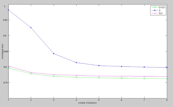
ZI is simply to take the initial values of all parameters as zero and then per-form the iteration steps, so it is called as ‘Zero Initialization’. This technique is employed as an initialization of SAGE algorithm for the measurement data scenario 68 and error versus iteration is presented in Figure 3.4 (blue line). The calculation of error is explained in the Section 3.5 and this calculation will be used in the other sections.

1 0.95 0.9 0.85 0.8 0.75

Figure 3.4: Error vs number of iteration. Iteration 1 represents initialization step for ZI (blue line), SICI (magenta line), DI-SICI (green line)

3.3.2

SIC Initialization

The other technique, a better one, is to use the Successive Interference Cancela-tion (SIC) method with the non-coherent ML estimaCancela-tion method [9]. Similar to SAGE iteration step, it has also E-step and M-step. These E-step and M-step are performed to find initial value of the parameters for all paths.

E-step

The expectation of admissible data of one path (xl,n,m,i(t)) can be found

by subtracting currently estimated path signals from observed data yn,m,i(t). Therefore expectation of admissible data for first path is the observed data itself, since no path is estimated currently. And general expression for expectation of admissible data is;

ˆ x[0]_l,n,m,i(t) = yn,m,i(t) − l−1 X l0₌₁ s(t; ˆΘ[0]_l0_,n,m,i) (3.22) M-step

Initially, lets define

hl,n,m,i(τl) =

R_Tsc

0 xˆ

[0]

l,n,m,i(t)u∗n,m,i(t − τl)dt (3.23)

kn,m,i(τl, νl) = exp{−j2πνlti,m,n}hl,n,m,i(τl) (3.24)

km(τl, νl) = hP_I i=1k1,m,i(τl, νl), . . . , P_I i=1kN,m,i(τl, νl) i_T (3.25)

Estimation formulas are as given below and details and derivations are pre-sented in [9]. ˆ τ_l[0] = arg maxτl hP_I i=1 P_N n=1 P_M m=1|hl,n,m,i(τl)|2 i (3.26) ˆ ν_l[0] = arg maxνl hP_N n=1 P_M m=1| P_I i=1kn,m,i(ˆτl[0], νl)|2 i (3.27) ˆ Ω[0]_Rx,l = arg maxΩ_Rx,l{ P_M m=1[|˜cHRx,v(ΩRx,l)km(ˆτ [0] l , ˆν [0] l )|2 + |˜cHRx,h(ΩRx,l)km(ˆτ [0] l , ˆν [0] l )|2 −2<{km(ˆτ_l[0], ˆν_l[0])H˜cRx,h˜cHRx,vkm(ˆτ [0] l , ˆν [0] l )T˜cHRx,h˜cRx,v}]} (3.28) ˆ Ω[0]_Tx,l = arg maxΩ_Tx,l|z(φTx,l, θTx,l, ˆφ [0] Rx,l, ˆθ [0] Rx,l, ˆτ [0] l , ˆν [0] l ; ˆx [0] l )| (3.29)

and polarization coefficients can be found with (3.17). In (3.28), ˜(.) denotes normalization.

This technique is also employed as an initialization of SAGE algorithm for the measurement data scenario 68 and error versus iteration is presented in Figure 3.4 (magenta line).

3.3.3

Delay Intuitive SIC Initialization

SIC Initialization (SICI) is better than Zero Initialization as seen in Figure 3.4, but SICI is slower than an iteration step of SAGE algorithm. To get better and faster initialization we propose a new way of SICI which is to set initial delays of paths intuitively instead of estimation.

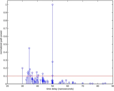
The idea is to set the delay of paths consistent with Impulse Response (RTsc

0 yn,m,i(t)u∗n,m,i(t − τ )dt) of the channels initially. That is to say, initial

de-lays of L paths are set by determining a delay range from Impulse Response (IR) which is below a certain limit of the peak value of IR (i.e. -20 dBpk (dB with respect to the peak value)). Therefore this technique changes only delay estimation of SIC Initialization (3.26). Since the time consuming part of SIC Initialization is delay estimation, this technique improves the computation time of the algorithm. This technique can be performed with the following steps:

1-Determine the number of paths to be estimated (L). 2-Determine a limit for IR value (i. e. -20 dBpk). 3-Find IR0_{(ς) = (}PI i=1 P_N n=1 P_M m=1| R_Tsc

0 yn,m,i(t)u∗n,m,i(t− ς)dt|2)/(NM I) where

ς value differs from 0 to Tscwith 5 nanoseconds intervals (the value of the interval

is optional)

4-Find the minimum and maximum value of ς (min(ς), max(ς)) which sets the

IR0 _{above the limit (-20 dBpk).}

5-Find VIR0 =

P_max(ς)

ς=min(ς)IR0(ς).

6-Find the number of paths for each ς with b(L.IR0_(ς))/V

IR0c and set the initial delay of the paths to the related ς and set the initial delays to ς values.

Then, path delays are initialized proportional to IR values as presented in Figure 3.5 and computation times of initialization techniques are reported in Table 3.1. As a result DI-SICI technique is slightly better for initialization than

SICI as seen in the Figure 3.4 and its computation time is significantly less compared to SICI. 0 50 100 150 200 250 300 350 400 450 500 −50 −40 −30 −20 −10 0 time (nanoseconds) dBpk a) 0 50 100 150 200 250 300 350 400 450 500 0 2 4 6 8 10 time (nanoseconds) number of paths b)

Figure 3.5: Explanation of DI-SICI technique: a-Blue line is the IR of a channel and red straight line is the -20 dBpk limit b-Determined number of paths for each ς.

Computation time of initialization

Initialization Technique of one path (seconds)

ZI 0.0

SICI 18.7

DI-SICI 4.4

Table 3.1: Comparison of computational expense of the initialization techniques. The techniques work in Matlab environment on an AMD Athlon 3800 processor.

3.4

Particle Swarm Optimization Algorithm for

the M-step of SAGE Algorithm

As we see from the formulas, the algorithm should search for the parameter values maximizing the likelihood function. Since the search domain is continuous this is a tedious operation requiring efficient search procedures. To this end we propose to use PSO to perform the optimization.

PSO is one of the evolutionary computation techniques developed for non-linear optimization problems with continuous valued parameters though it can also be used with discrete variables [11]. The procedure is based on researches on swarms like bees and bird flocking and inspired by social behavior of swarms [11]. This procedure is simple and its computation time is short.

According to the biological research, swarms find their food collectively not individually; information is shared within the members of swarm. In the swarm, each member’s position in the space and its information are known, so each member’s position and velocity (change of the position of the member in an iteration) in the space are modified.

for each member

Initialize the velocity and the position in the space end

for each member Calculate fitness value

Compare the fitness value with pbest at hand and set the pbest to the better one end

for each member

Calculate the velocity of the member using (3.30) Update the position of the member in the space using (3.31)

end

while convergence is not achieved

Choose the best pbest among the pbests of the members as gbest

end

Figure 3.6: The pseudo code of the PSO.

Swarm movement optimizes a certain objective function. All of the members of the swarm have fitness values which are evaluated by the objective function to be optimized, and have change of positions per iteration in the space. Each member knows its best value (pbest) among the previous positions of its own in the space. Moreover, each member knows the best value at hand in the swarm, i.e. the global best (gbest), among pbests. Each member wants to change its position in the space according to its change of position per iteration and the distance to pbest and gbest. The pseudo code of the algorithm is explained in the Figure 3.6. Velocity and position of each member can be calculated by the following equations:

∆ = w ∗ ∆ + c1 ∗ rand ∗ (pbest − present)

present = present + ∆. (3.31)

Here ∆ is the change of position of the member for an iteration, w is the scaling factor, present is the current member’s position in the space, rand is a random number between (0,1). c1, c2 are learning factors, usually taken as

c1 = c2 = 2.

3.4.1

Performance of SAGE with PSO

To investigate the performance of SAGE algorithm together with PSO, the mea-surement data, explained in Chapter 2, is used and PSO parameters are chosen as in Table 3.2.

number of swarm members 10

w 0.1

initial value of ∆ (delay) 1 nanosecond/iteration

initial value of ∆ (angles) 1 degree/iteration

initial value of ∆ (Doppler frequency) 0.1 hertz/iteration

Table 3.2: PSO parameters employed.

The channel parameters are estimated by SAGE algorithm using three dif-ferent search procedures: PSO, Brute Force search and fminsearch. Brute Force Search means sampling the cost function within the reference domain and then choosing maximum of that function and fminsearch is an unconstrained nonlinear optimization function in the Matlab Optimization Toolbox [12].

We observed that estimated the parameters nearly the same for three search procedures. Table 3.3 shows the computation time of search procedures both at initialization and SAGE iterations. It also illustrates that PSO’s computation time for each iteration is significantly better than other methods.

Estimation of Computation time of

one path with one iteration (seconds)

Initialization 192

Brute Force Search

Sage iteration 101 Initialization 20 fminsearch Sage iteration 15.5 Initialization 18.7 PSO Sage iteration 9.2

Table 3.3: Computational expense of the algorithm compared with other meth-ods. The algorithm works in Matlab environment on an AMD Athlon 3800 processor.

3.5

Error Calculation

In this work, to see the difference between observed data (y(t))and reconstructed data (y(t)R_{) the error is calculated as explained below.}

1-Estimate all channel parameters for L paths

2-Reconstruct the paths (sl,n,m,i(t)R) with estimated parameters using (3.10) for

all channels of employed cycles

3-Find Rx antenna output for all channels using yn,m,i(t)R =

P_L

l=1sl,n,m,i(t)R

4-Find error using

error = [ P_I i=1 P_M m=1 P_N n=1{ R_Tsc 0 |yn,m,i(t)R− yn,m,i(t)|dt}] [PI_i=1PM_m=1PN_n=1{RTsc 0 |yn,m,i(t)|dt}] . (3.32)

Chapter 4

NUMERICAL RESULTS

In this chapter, the measurement data are analyzed using SAGE algorithm in combination with the aforementioned techniques. The results for each scenario are presented in the following sections. The results consist of analysis of scenario data, illustration of estimated parameters and the error analysis.

4.1

Scenario 68

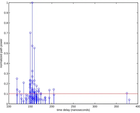
For this scenario, Tx and Rx antenna arrays are located as shown in Figure 4.1. Table 4.1 lists the parameters employed in the SAGE algorithm. The results obtained from scenario 68 are presented in the figures shown below. Figures 4.2 and 4.3 show the delay range of paths. Figure 4.2 presents impulse response of a channel (m=10, n=22) and average value of all channels. The impulse responses are normalized with respect to the peak value, so the vertical axis is shown in dBpk. The average value is determined after the normalization of each impulse response. It can be seen that delay range of averaged impulse response is 25-100 nanoseconds for -30 dBpk limit. Figure 4.3 shows impulse response of all channels in color code. It is understood from the figure that delay range

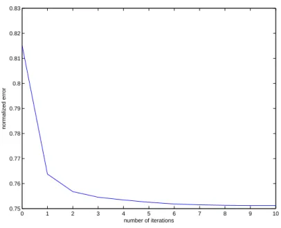
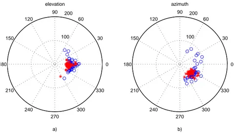
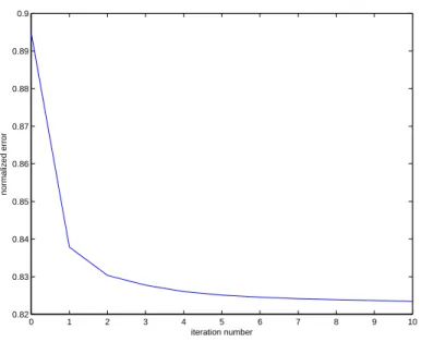
of paths for all channels is nearly the same around 30-100 nanoseconds. With these observations, the paths are determined in these ranges and the results are presented in Figures 4.4, 4.5 and 4.6. As listed in 4.1, 79 paths are estimated with 10 iterations. Figure 4.4 presents power delay profile (pdf) of estimated paths. It is seen that some paths have low power and one tenth of the power of the most dominant path is taken as a limit for dominant paths, so delay range of dominant paths is 30-50 nanoseconds. Angles of departure and arrival are shown in Figures 4.5 and 4.6 in polar coordinates where the radial axis represents the time delay of each path. It is understood that elevation angles have narrow range because of the floor height and antenna radiation patterns. Additionally, azimuth angles of departure have wider range compared to azimuth angles of arrival, because of the antenna radiation patterns and scenario type (Room to Corridor). Then, estimated parameters are employed to reconstruct the signal at the receiver antenna array and comparison of real and imaginary parts of reconstructed signal and observed signal is shown in Figures 4.7 and 4.8, respectively for channel number 1. The comparison is done due to the knowledge of SNR ≥ 20dB. It can be seen that they do not have exact match, but they are similar. Finally, Figure 4.9 shows error change with respect to iteration number. The iteration number 0 refers to initialization step and error decreases with iteration number.

number of employed measurement cycles 2

number of estimated paths 79

number of iterations performed 10

Figure 4.1: Positions of Tx and Rx antenna arrays for scenario 68. 0 50 100 150 200 250 300 350 400 450 500 −70 −60 −50 −40 −30 −20 −10 0 time (nanoseconds) Impulse Response (dBpk)

averaged impulse response of all channels impulse response of channel number 342 −30 dBpk

Figure 4.2: Impulse response of channel number 342 (blue line), all channels averaged (red line) and dBpk limits for scenario 68.

channel number time (nanoseconds) 200 400 600 800 1000 1200 1400 1600 50 100 150 200 250 300 350 400 450 500 −15 −14 −13 −12 −11 −10 −9 −8 −7 −6 −5

Figure 4.3: Absolute value of impulse response of all channels versus time for scenario 68. 20 30 40 50 60 70 80 90 0 0.1 0.2 0.3 0.4 0.5 0.6 0.7 0.8 0.9 1

time delay (nanoseconds)

normalized path power

Figure 4.4: Power delay profile of estimated 79 Paths and the constant value is the assumed threshold for dominant paths for scenario 68.

50 100 30 210 60 240 90 270 120 300 150 330 180 0 elevation a) 50 100 30 210 60 240 90 270 120 300 150 330 180 0 azimuth b)

Figure 4.5: Angle of departures of estimated paths both azimuth and elevation versus time delay (o) and Electrobit Testing results (*) for scenario 68.

50 100 30 210 60 240 90 270 120 300 150 330 180 0 elevation a) 50 100 30 210 60 240 90 270 120 300 150 330 180 0 azimuth b)

Figure 4.6: Angle of arrivals of estimated paths both azimuth and elevation versus time delay (o) and Electrobit Testing results (*) for scenario 68.

0 50 100 150 200 250 300 350 400 450 500 −20 −15 −10 −5 0 5 10 15 time (nanoseconds)

real part of signals

Figure 4.7: Comparison of the real part of reconstructed signal (blue line) and observed signal (dashed red line) for scenario 68.

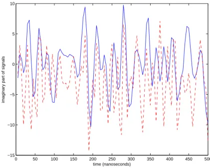
0 50 100 150 200 250 300 350 400 450 500 −15 −10 −5 0 5 10 time (nanoseconds)

imaginary part of signals

Figure 4.8: Comparison of the imaginary part of reconstructed signal (blue line) and observed signal (dashed red line) for scenario 68.

0 1 2 3 4 5 6 7 8 9 10 0.75 0.76 0.77 0.78 0.79 0.8 0.81 0.82 0.83 number of iterations normalized error

Figure 4.9: Error change with respect to iteration number for scenario 68.

4.2

Scenario 82

In this scenario, observations and results are found in similar ways with scenario 68. From the results, it can be seen that the power delay profile of dominant paths is wider than scenario 68, because of the antenna separation and antenna position. The elevation angles are similar since the measurement is done on the same floor. Additionally, because of the antenna positions, azimuth angles have narrower range compared to scenario 68. Figures 4.14 and 4.15 show the real and imaginary part comparison of reconstructed and observed signal, it can be seen that there is better match compared to scenario 68, so the error is smaller as shown in Figure 4.16.

number of employed measurement cycles 2

number of estimated paths 64

number of iterations performed 10

delay range (-30 dBpk) [45,200] nanoseconds

Figure 4.10: Positions of Tx and Rx for scenario 82. 50 60 70 80 90 100 110 120 0 0.2 0.4 0.6 0.8 1

time delay (nanoseconds)

normalized path power

Figure 4.11: Power delay profile of estimated 64 paths and the constant value is the assumed threshold for dominant paths for scenario 82.

100 200 30 210 60 240 90 270 120 300 150 330 180 0 elevation a) 100 200 30 210 60 240 90 270 120 300 150 330 180 0 azimuth b)

Figure 4.12: Angle of departures of estimated paths both azimuth and elevation versus time delay (o) and Electrobit Testing results (*) for scenario 82.

100 200 30 210 60 240 90 270 120 300 150 330 180 0 elevation a) 100 200 30 210 60 240 90 270 120 300 150 330 180 0 azimuth b)

Figure 4.13: Angle of arrivals of estimated paths both azimuth and elevation versus time delay (o) and Electrobit Testing results (*) for scenario 82.

0 50 100 150 200 250 300 350 400 450 500 −15 −10 −5 0 5 10 time (nanoseconds)

real part of signals

Figure 4.14: Comparison of real part of reconstructed signal (blue line) and observed signal (dashed red line) for scenario 82.

0 50 100 150 200 250 300 350 400 450 500 −5 0 5 10 time (nanoseconds)

imaginary part of signals

Figure 4.15: Comparison of imaginary part of reconstructed signal (blue line) and observed signal (dashed red line) for scenario 82.

0 1 2 3 4 5 6 7 8 9 10 0.82 0.83 0.84 0.85 0.86 0.87 0.88 0.89 0.9 iteration number normalized error

Figure 4.16: Error change with respect to iteration number for scenario 82.

4.3

Scenario 72

From the results, it can be seen that the power delay profile, dominant paths are fewer than scenario 68 and 82, because of the scenario type (Corridor to corridor LOS). Additionally, because of the antenna positions and the scenario type, azimuth angles have narrower range compared to scenario 82.

number of employed measurement cycles 2

number of estimated paths 74

number of iterations performed 7

delay range (-30 dBpk) [70,225] nanoseconds

Figure 4.17: Positions of Tx and Rx for scenario 72. 60 80 100 120 140 160 180 200 220 0 0.1 0.2 0.3 0.4 0.5 0.6 0.7 0.8 0.9 1

time delay (nanoseconds)

normalized path power

Figure 4.18: Power delay profile of estimated 74 paths and the constant value is the assumed threshold for dominant paths for scenario 72.

100 200 30 210 60 240 90 270 120 300 150 330 180 0 elevation a) 100 200 30 210 60 240 90 270 120 300 150 330 180 0 azimuth b)

Figure 4.19: Angle of departures of estimated paths both azimuth and elevation versus time delay (o) and Electrobit Testing results (*) for scenario 72.

100 200 30 210 60 240 90 270 120 300 150 330 180 0 elevation a) 100 200 30 210 60 240 90 270 120 300 150 330 180 0 azimuth b)

Figure 4.20: Angle of arrivals of estimated paths both azimuth and elevation versus time delay (o) and Electrobit Testing results (*) for scenario 72.

0 50 100 150 200 250 300 350 400 450 500 −20 −15 −10 −5 0 5 10 time (nanoseconds)

real part of signals

Figure 4.21: Comparison of real part of reconstructed signal (blue line) and observed signal (dashed red line) for scenario 72.

0 50 100 150 200 250 300 350 400 450 500 −20 −15 −10 −5 0 5 10 15 time (nanoseconds)

imaginary part of signals

Figure 4.22: Comparison of imaginary part of reconstructed signal (blue line) and observed signal (dashed red line) for scenario 72.

0 1 2 3 4 5 6 7 0.74 0.745 0.75 0.755 0.76 0.765 0.77 0.775 0.78 iteration number normalized error

Figure 4.23: Error change with respect to iteration number for scenario 72.

4.4

Scenario 73

From the results, it can be seen that the power delay profile of dominant paths is wider than scenario 72, because of the scenario type (Corridor to corridor NLOS). Additionally, because of the Tx antenna position, azimuth angles of departure have wider range compared to scenario 72.

number of employed measurement cycles 2

number of estimated paths 86

number of iterations performed 7

delay range (-30 dBpk) [110,450] nanoseconds

Figure 4.24: Positions of Tx and Rx for scenario 73. 100 150 200 250 300 350 400 0 0.1 0.2 0.3 0.4 0.5 0.6 0.7 0.8 0.9 1

time delay (nanoseconds)

normalized path power

Figure 4.25: Power delay profile of estimated 86 paths and the constant value is the assumed threshold for dominant paths for scenario 73.

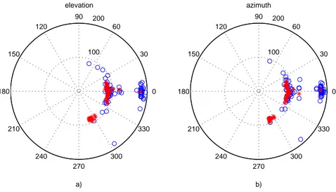
200 400 30 210 60 240 90 270 120 300 150 330 180 0 elevation a) 200 400 30 210 60 240 90 270 120 300 150 330 180 0 azimuth b)

Figure 4.26: Angle of departures of estimated paths both azimuth and elevation versus time delay (o) and Electrobit Testing results (*) for scenario 73.

200 400 30 210 60 240 90 270 120 300 150 330 180 0 elevation a) 200 400 30 210 60 240 90 270 120 300 150 330 180 0 azimuth b)

Figure 4.27: Angle of arrivals of estimated paths both azimuth and elevation versus time delay (o) and Electrobit Testing results (*) for scenario 73.

0 50 100 150 200 250 300 350 400 450 500 −6 −4 −2 0 2 4 6 time (nanoseconds)

real part of signals

Figure 4.28: Comparison of real part of reconstructed signal (blue line) and observed signal (dashed red line) for scenario 73.

0 50 100 150 200 250 300 350 400 450 500 −6 −4 −2 0 2 4 6 time (nanoseconds)

imaginary part of signals

Figure 4.29: Comparison of imaginary part of reconstructed signal (blue line) and observed signal (dashed red line) for scenario 73.

0 1 2 3 4 5 6 7 0.61 0.62 0.63 0.64 0.65 0.66 0.67 0.68 0.69 iteration number normalized error

Figure 4.30: Error change with respect to iteration number for scenario 73.

4.5

Scenario 79

From the results, it can be seen that the results are similar with scenario 68, since the scenario types are the same (Room to corridor NLOS).

number of employed measurement cycles 2

number of estimated paths 112

number of iterations performed 7

delay range (-30 dBpk) [60,220] nanoseconds

Table 4.5: Employed SAGE parameters for scenario 79.

60 80 100 120 140 160 180 200 0 0.1 0.2 0.3 0.4 0.5 0.6 0.7 0.8 0.9 1

time delay (nanoseconds)

normalized path power

Figure 4.32: Power delay profile of estimated 112 paths and the constant value is the assumed threshold for dominant paths for scenario 79.

100 200 30 210 60 240 90 270 120 300 150 330 180 0 elevation a) 100 200 30 210 60 240 90 270 120 300 150 330 180 0 azimuth b)

Figure 4.33: Angle of departures of estimated paths both azimuth and elevation versus time delay (o) and Electrobit Testing results (*) for scenario 79.