Zayıf tekil çekirdekli lineer integro diferansiyel denklemlerin bir sınıfının chebyshev seri çözümleri

* Corresponding Author

Chebyshev Series Solutions for a Class of System of Linear Integro-Differential Equations with Weakly Singular Kernel

Yalçın ÖZTÜRK*

Muğla Sıtkı Koçman University, Ula Ali Koçman Vocational School, Muğla, Turkey yozturk@mu.edu.tr, ORCID: 0000-0002-4142-5633

Abstract

In this study, a numerical algorithm for solving a class of system of linear integro differential equations with weakly singular kernel is presented. This algorithm is based on polynomial approximation and collocation method, using the first kind Chebyshev polynomial basis. This method transforms the equations and the given conditions into matrix equation which corresponds to a system of linear algebraic equation. To show the validity and applicability of the numerical method some experiments are examined. Present method is compared some numerical methods.

Keywords: Singular system of integro-differential equations, Weakly singular

kernel, Abel’s equation, Collocation method, Chebyshev polynomials

Zayıf Tekil Çekirdekli Lineer İntegro Diferansiyel Denklemlerin Bir Sınıfının Chebyshev Seri Çözümleri

Öz

Bu çalışmada, zayıf tekil çekirdekli lineer integro diferansiyel denklemlerin bir sınıfı için bir nümerik algoritma sunulacaktır. Bu algoritma birinci tip Chebyshev polinom bazı yardımıyla polinom yaklaşımı ve sıralama metodunu temel almaktadır. Bu metot verilen denklem ve koşulları bir matris denklemine dönüştürür. Nümerik metodun uygulanabilirliğini ve doğruluğunu göstermek amacıyla bazı örnekler incelenecektir. Sunulan metot diğer metotlar ile kıyaslanmıştır.

Adıyaman University Journal of Science https://dergipark.org.tr/en/pub/adyujsci

DOI: 10.37094/adyujsci.508986

ADYUJSCI

9 (2) (2019) 314-328

Anahtar Kelimeler: İntegro-diferansiyel denklemlerin singular sistemleri, Zayıf

tekil çekirdek, Abel denklemi, Sıralama metodu, Chebyshev polinomları

1. Introduction

Applications in many important fields, like fracture mechanics, elastic contact problems, the theory of porous filtering and combined infrared radiation and molecular conduction [1-4], contain integral and integro-differential equations with singular kernel. Singular integral and integro-differential equations are usually difficult to solve analytically so it is required to obtain the approximate solution and the aim in the present research is to develop an accurate as well as easy to implement numerical solution scheme to treat such equations.

These type equations have been solved numerically by some authours. We can give some studies in literature [5-17].

We consider the class of system of linear integro-differential eqeuations with weakly singular kernel

( ) ( ) ( ) ( ) 0 0 0 ) ( _{dx f t} x t x y t y t P _j t j j n p m q p q j pq + -=

ò

åå

= = l , j =0,1,!m (1) with conditions n _j r m p r p j rpy t c =l

åå

-= = 1 0 0 ) ( _{( ) (2)} wheref_j(t) and Pj (t)

pq are analytic functions, c and rpj l are constant. For j q=0, Eq. (1) is a nonsystem integro-differential equation and is Abel’s equation with convenient coefficients. We construct to the shifted Chebyshev series solutions that is;

å

= = N r r j r N j t a T t y 0 ) ( ) ( (3)

where T_r(t) denotes the Chebyshev polynomials of the first kind, aj (0 r N)

r £ £ are

The Chebyshev polynomials T_r(t) of the first kind are the polynomials in t of degree r, defined by relation [18, 19]

q n t

T_r( )=cos , when t =cosq.

If the range of the variable t is the interval [-1,1], the range the corresponding variables q can be taken [0,p . These polynomials have the following properties [18, ] 19]:

i) The Chebyshev polynomials with degree r+1 has absolutly complete r+1 real zeroes which is called The Chebyshev-Gaus nodes on the interval [-1,1] and these roots compute as ) 1 ( 2 ) 1 ) ( 2 ( cos + + -= r i r t_i p , i=0,1,!,N. (4)

ii) The Chebyshev polynomials with degree r is ortogonal on [-1,1] together with

the weight function 2

1 2₎ 1 ( ) (t = -t -w .

iii) The passing equation between the powers _tn _{and the Chebyshev polynomials} ) (t T_r is

å

= + -÷÷ ø ö çç è æ -= r s s r r _{T t} s r r t 0 2 1 2 2 _{2 ( ), (5)}

å

= + -+ ÷÷ ø ö çç è æ -+ = r s s r r _{T t} s r r t 0 1 2 2 1 2 ₂ 2 1 _{( ). (6)}

2. Fundamental Matrix Relations

In this section, we convert the part of Eq. (1) and conditions Eq. (2) into the matrix form. Using the Eq. (3), we have the matrix relation of solutions and its derivatives as:

N j j t t y ( )=T )( A ,

( )

N s s j j t t y ( )( )₌T( )( )A _{j =0,1,!m,} (7) where

)] ( ... ) ( ) ( [ ) (t = T₀ t T₁ t T_N t T T j N j j j _{[a a ...a ]} 1 0 = A

By using the expression (5) and (6) and taking r =0,1,!,N we find the corresponding matrix relation as follows

_(Y(t))T _=D(T(t))T _{and Y(t)=T(t)D}T_{, (8)} where ] 1 [ ) ( N t t t = ! Y ,

and for odd N,

ú ú ú ú ú ú ú ú ú ú ú û ù ê ê ê ê ê ê ê ê ê ê ê ë é ÷÷ ø ö çç è æ ÷÷ ø ö çç è æ -÷÷ ø ö çç è æ ÷÷ ø ö çç è æ ÷÷ ø ö çç è æ ÷÷ ø ö çç è æ = -N N N N 1 1 1 0 1 2 0 0 2 / ) 1 ( 0 0 2 0 2 0 2 1 2 2 1 0 0 2 0 1 0 0 0 0 2 0 0 2 1 ! " # " " " ! ! ! D , for even N, ú ú ú ú ú ú ú ú ú ú ú û ù ê ê ê ê ê ê ê ê ê ê ê ë é ÷÷ ø ö çç è æ ÷÷ ø ö çç è æ -÷÷ ø ö çç è æ ÷÷ ø ö çç è æ ÷÷ ø ö çç è æ ÷÷ ø ö çç è æ ÷÷ ø ö çç è æ = -N N N N N N N N _{1 1 1} 1 1 0 1 2 0 2 2 / ) 2 ( 0 2 2 / 2 1 0 2 0 2 0 2 1 2 2 1 0 0 2 0 1 0 0 0 0 2 0 0 2 1 ! " # " " " ! ! ! D .

Then, by taking into account (8) we obtain

T t t) ( )( ) ( _{=Y D}-1 T and _(T(t))(q) _=Y(q)_(t)(D-1₎T _{, q=0,1,...,n. (9)} To obtain the matrix _Y(s)(t) _{in terms of the matrixY(t), we can use the following relation:}

_Y(q)_(t)=Y(t)(BT₎q_{, (10)} where _{( )}0 _{( 1) ( 1)} + ´ + = _{n n} T _I B and ú ú ú ú ú ú û ù ê ê ê ê ê ê ë é = 0 0 0 0 0 0 2 0 0 0 0 1 0 0 0 0 N ! ! ! ! ! ! ! ! B .

Consequently, by substituting the matrix form (9) and (10) into (7), we get the matrix representation of approximate solution and its derivatives as follows:

( )

N q

( )

T q T j

j t t

y ( )_{( )=}Y_{( )}B ₍D ₎-1A _{. (11)} On the other hand, the matrix representation of the conditions Eq. (2) are given by matrix relation as:

n

( )

_j r m p p T r T j rp t c =l

åå

-= = -1 0 0 1 ) ( ) ( B D A Y . (12)

For the part

_ò

-t j j dx x t x y 0 ) (

l , we have the following equation [7]

ò

+ G + G = -+ t N N N x N dx x t x 0 ) 2 1 ( ) 2 3 ( ) 1 ( p

and so, we get

T j j t j T t j j j dt t x t t dx x t x y A D Q A D Y ) )( ( ) ( ) ( ) ( ₁ 0 1 0 -- ₌ ÷÷ ø ö çç è æ -=

-ò

l

ò

l l , (13) where ú ú ú ú û ù ê ê ê ê ë é + G + G G G G G = x +N N N x x t 2 1 2 3 2 1 ) 2 3 ( ) 1 ( ) 2 5 ( ) 2 ( ) 2 3 ( ) 1 ( ) ( p p ! p Q .

3. Description Method

In this chapter, we present the fundamental matrix equation which give us the matrix form of Eq. (1). To obtain the matrix form of Eq. (1), If Eq. (11) is put into Eq. (1), we have ( ) ( )

( )

( ) ( ) ( ) 0 1 0 0 t f dx x t x y t t P _j t j j q T q T n p m q j pq + -=

_ò

åå

-= = l A D B Y , j=0,1,!m (14)

then, it can be written as:

P Y_____B D Q D_÷÷A=F ø ö çç è æ

-å

= m q q q j t t 0 _____ ) ( ) ( l , (15) where ú ú ú ú û ù ê ê ê ê ë é = ) ( 0 0 0 ) ( 0 0 0 ) ( ) ( _____ t t t t Y Y Y Y ! " # " " ! ! ,

( )

( )

( )

úú ú ú ú û ù ê ê ê ê ê ë é = q T q T q T q B B B B ! " # " " ! ! 0 0 0 0 0 0 , ú ú ú ú ú û ù ê ê ê ê ê ë é = -1 1 1 ) ( 0 0 0 ) ( 0 0 0 ) ( T T T D D D D ! " # " " ! ! , ú ú ú ú ú û ù ê ê ê ê ê ë é = ) ( ) ( ) ( ) ( ) ( ) ( ) ( ) ( ) ( ) ( 1 0 1 1 1 1 0 0 0 1 0 0 t P t P t P t P t P t P t P t P t P t m qn m q m q qn q q qn q q q ! " # " " ! ! P , ú ú ú ú û ù ê ê ê ê ë é = ) ( 0 0 0 ) ( 0 0 0 ) ( ) ( _____ t t t t Q Q Q Q ! " # " " ! ! , ú ú ú ú û ù ê ê ê ê ë é = ) ( ) ( ) ( 1 0 t f t f t f m ! F , ú ú ú ú ú û ù ê ê ê ê ê ë é = m A A A A ! 1 0 ,

If the Chebyshev-Gauss grid nodes are put into Eq. (14), the matrix form of the Eq. (1) is obtained P YB D QD_÷÷A=___F ø ö çç è æ

-å

= ___ 0 ___ ____ j m q q q l , (16)

ú ú ú ú ú û ù ê ê ê ê ê ë é = ______ ______ 1 ______ 0 ___ ) ( 0 0 0 ) ( 0 0 0 ) ( N t t t Y Y Y Y ! " # " " ! ! , ú ú ú ú ú û ù ê ê ê ê ê ë é = qN q q q P P P P ____ ! " # " " ! ! 0 0 0 0 0 0 1 0 , ú ú ú ú ú û ù ê ê ê ê ê ë é = ______ ______ 1 ______ 0 ___ ) ( 0 0 0 ) ( 0 0 0 ) ( N t t t Q Q Q Q ! " # " " ! ! , ú ú ú ú û ù ê ê ê ê ë é = N F F F F ! 1 0 ___ , where ú ú ú ú û ù ê ê ê ê ë é = ) ( 0 0 0 ) ( 0 0 0 ) ( ) ( ______ i i i i t t t t Y Y Y Y ! " # " " ! ! , ú ú ú ú ú û ù ê ê ê ê ê ë é = ) ( 0 0 0 ) ( 0 0 0 ) ( i q i q i q qi t t t P P P P ! " # " " ! ! , ú ú ú ú û ù ê ê ê ê ë é = ) ( 0 0 0 ) ( 0 0 0 ) ( ) ( ______ i i i i t t t t Q Q Q Q ! " # " " ! ! , ú ú ú ú û ù ê ê ê ê ë é = ) ( ) ( ) ( 1 0 i m i i i t f t f t f ! F ,

where the dimension of matrices ___Y, B_q, D , P ,____q ___Q diagonal matrices and the dimension of these matrices are m(N +1)´m(N +1), P_k(t), B are _k (m+1)´(s+1) and

___

F is m(N+1)´1.

Hence, the matrix equation (16) corresponding to Eq. (1) can be written in the form WA=___F or _êëéW; F____úûù, (17) where

å

= = m q 0 q q ___ ____ D B Y P W .

Moreover, the matrix form for conditions can be written as

UA=G, (18) where for k =0,1,!,m, l =0,1,!,m(N+1), ú ú ú ú ú ú û ù ê ê ê ê ê ê ë é = = m kl u U U U U U ! " # " " " ! ! ! 0 0 0 0 0 0 0 0 0 0 0 0 ] [ ₂ 1 0 , ú ú ú ú ú ú û ù ê ê ê ê ê ê ë é = m l l l l ! 2 1 0 G , and

( )

_{( )} 1 ) ( -= j T r T rp j c Y t B D U , j=0,1,!,m.

If the condition matrix Eq. (18) relocate by the last n rows of the matrix Eq. (17) to get the approximate solution of system of linear integro-differential equations with weakly singular kernel Eq. (1) with the conditions Eq. (2) by Chebyshev polynomials, we obtain the augmented matrix:

____WA= F• , (19) where ú ú ú ú ú ú ú ú ú û ù ê ê ê ê ê ê ê ê ê ë é = + ´ + ´ + ´ -´ -´ -+ ´ + ´ ) 1 ( 1 0 ) 1 ( 0 01 00 ) 1 ( ) 1 ( 1 ) 1 ( 0 ) 1 ( ) 1 ( 1 11 10 ) 1 ( 0 01 00 ___ N m m m m N m N m N m N m N m N m N m u u u u u u w w w w w w w w w ! " ! " " ! ! " # " " ! ! W and

ú ú ú ú û ù ê ê ê ê ë é = -• G F F F 1 0 N ! .

Therefore, Eq. (19) give us a algebraic systems which include m(N +1)´m(N+1) linear algebraic equations with m(N +1) unknown Chebyshev coefficients. If ____W is invertible, then it can be written _A=(W___₎-1_F•_{. Thus, the matrix A (thereby the}

coefficients matrix_{A ,} j _{j 0,1, ,m} !

= ) is uniquely determined.

4. Test Problems

In this section, we give five test problem corresponding to equation (1) to demonstrate the efficiency of proposed method. Examples 1 and 2 is are given systems of integro-differential equations, 3 and 4 are Abel’s equations. All numerical scheme is calculated by using Maple 15. The absolute errors in Tables are the values of

) ( ) (t y t y N N j j

e = - , those at selected points.

Example 1. Let us consider the following singular integro-differential equation

3 / 4 3 0 0 1 0 ' 0 3 4 1 ) ( ) ( ) ( ) ( dx t t t x t x y t ty t y t y t -+ + -= -+

ò

,

ò

+ + -= + + t dx t t t x t x y t y t ty t y 0 2 / 5 2 1 1 0 ' 1 15 16 2 2 ) ( ) ( ) ( ) ( ,

with subject to conditions

0 ) 0 ( ) 0 ( ₁ 0 = y = y ,

with eaxact solutions y₀(t)=t ve 2 1(t) t

y = . For N =5, we seek the approximate solutions, we have the fundamental matrix equation from Eq.(16)

P YD P YB D QD÷A=___F ø ö ç è æ _{+ -}___ 1 ___ ____ 1 ___ ____ 0 , (20) with

ú û ù ê ë é = 1 0 0 1 ) ( 1 t P , _ú û ù ê ë é -= 1 1 ) ( 0 _t t t P , ú ú ú ú û ù ê ê ê ê ë é G G G G G G G G G G = 2 9 2 7 2 5 2 3 2 1 ) 2 11 ( ) 5 ( ) 2 9 ( ) 4 ( ) 2 7 ( ) 3 ( ) 2 5 ( ) 2 ( ) 2 3 ( ) 1 ( ) (t p x p x p x p x p x Q ,

and with collocation points, we have

ú ú ú ú ú ú ú ú û ù ê ê ê ê ê ê ê ê ë é = 05 04 03 02 01 00 0 0 0 0 0 0 0 0 0 0 0 0 0 0 0 0 0 0 0 0 0 0 0 0 0 0 0 0 0 0 0 P P P P P P P___ , ú ú ú ú ú ú ú ú û ù ê ê ê ê ê ê ê ê ë é = 15 14 13 12 11 10 1 0 0 0 0 0 0 0 0 0 0 0 0 0 0 0 0 0 0 0 0 0 0 0 0 0 0 0 0 0 0 P P P P P P P ___ , ú ú ú ú ú ú ú ú û ù ê ê ê ê ê ê ê ê ë é = 5 4 3 2 1 0 ___ F F F F F F F , ú û ù ê ë é = B B B 0 0 ____ 1 , ú û ù ê ë é = -1 _-1 ) ( 0 0 ) ( T T D D D , , _ú û ù ê ë é = ₁0 A A A and where ú û ù ê ë é = 1 0 0 1 ) ( 1i t P , _ú û ù ê ë é -= 1 1 ) ( 0 i i i i _t t t P , ú ú ú û ù ê ê ê ë é -+ -+ = 2 / 5 2 3 / 4 3 15 16 2 2 3 4 1 i i i i i i i t t t t t t F , ú ú ú ú û ù ê ê ê ê ë é G G G G G G G G G G = 2 9 2 7 2 5 2 3 2 1 ) 2 11 ( ) 5 ( ) 2 9 ( ) 4 ( ) 2 7 ( ) 3 ( ) 2 5 ( ) 2 ( ) 2 3 ( ) 1 ( ) (t_i p t_i p t_i p t_i p t_i p t_i Q , ú ú ú ú ú ú ú ú û ù ê ê ê ê ê ê ê ê ë é -= -16 0 0 0 0 0 0 8 0 0 0 0 20 0 4 0 0 0 0 8 0 2 0 0 5 0 3 0 1 0 0 1 0 1 0 1 ) (_DT 1 , ú ú ú ú ú ú ú ú û ù ê ê ê ê ê ê ê ê ë é = 0 0 0 0 0 0 5 0 0 0 0 0 0 4 0 0 0 0 0 0 3 0 0 0 0 0 0 2 0 0 0 0 0 0 1 0 T B .

Moreover, the matrix form for conditions can be written as:

ú û ù ê ë é = ú û ù ê ë é ú û ù ê ë é º ú û ù ê ë é 0 0 0 0 ) 0 ( ) 0 ( 1 0 0 0 1 0 A A U U y y .

Solving the new augmented matrix based on conditions, truncated Chebyshev coefficients matrix are obtained as:

ú ú ú ú ú ú ú ú û ù ê ê ê ê ê ê ê ê ë é = 0 0 0 0 5 . 0 5 . 0 0 A and ú ú ú ú ú ú ú ú û ù ê ê ê ê ê ê ê ê ë é = 0 0 0 125 . 0 5 . 0 375 . 0 1 A .

Hence, the solutions of the problem for N =5 become y5(t)=t

0 and

2 5

1(t) t

y = which

are the exact solution of problem.

Example 2. Let us consider the following the systems of Volterra

integro-differential equation with weakly singular kernel

ò

+ -= + + + -t t _{dx f t} x t x y t y t y e t y t y 0 0 0 1 0 ' 1 ' 0 ( ) ) ( ) ( ) ( ) ( ) ( ,

ò

+ -= -+ - -t t _{dx f t} x t x y t y e t y t y t y 0 1 1 1 0 ' 1 ' 0 ( ) ) ( ) ( ) ( ) ( ) ( , where

ò

-+ + = t t t x _dx x t x e t t e t e t f 0 0 ) cos( ) cos( ) sin( ) cos( 2 ) ( ,

ò

-= t t t x _dx x t x e t t e t e t f 0 1 ) sin( ) sin( ) sin( 2 ) cos( ) ( ,

with y₀(0)=1 and y₁(0)=0 and exact solutions are y₀(t)₌etcos(t) _and )

sin( )

(

1 t e t

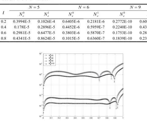
y ₌ t _{. Approximately solving these systems by present method for N =5,6,9} we obtain the numerical results in Table 1. Moreover, we display the absolute errors for

10 , 9 , 6 , 5 =

Table 1. Absolute errors for various N

t 0 N =5 N =6 N =9 e N 1 e N 0 e N 1 e N 0 e N 1 e N

0.2 0.3994E-5 0.1026E-4 0.6405E-6 0.2181E-6 0.2772E-10 0.6070E-10 0.4 0.178E-5 0.2896E-5 0.4452E-6 0.5959E-7 0.2240E-10 0.4397E-10 0.6 0.2981E-5 0.6477E-5 0.3803E-6 0.5870E-7 0.1753E-10 0.2801E-10 0.8 0.4341E-5 0.8624E-5 0.1015E-5 0.6360E-7 0.1839E-10 0.2368E-10

Figure 1. Comparison of the absolute errors for y₀(t) in Ex. 2

Figure 2. Comparison of the absolute errors for y₁(t) in Ex. 2

Example 3. We consider the Volterra integro-differential equation with weakly

singular kernel [7]

ò

= -+ + x f x t x t y x y x y 0 ) ( ) ( '' 1 ) ( ) ( '' p with y(0)= y'(0)=1. Here, if f(x) is chosen as

p x x

x 4

3_{+ +} 2 _{+ , the exact solution is}

2

4 3 2 4(x) 1 t t 0.13521E 19t 0.31881E 20t y = + + + - - - .

In [12], it is obtained the approximate solution for N =5 in [14]

5 2 _{0.1 18} 1 ) (x x x E x y = + + +

-and we compare the absolute errors present method -and Berstein series solution [12] in Table 2.

Table 2. Comparision of Berstein method and present method x Exact solution Işik [14] ) 5 (N= Present met. (N=4) 0.0 1.00 0.000E-0 0.200E-19 0.2 1.24 0.355E-18 0.200E-19 0.4 1.56 0.532E-18 0.000E-00 0.6 1.96 0.700E-18 0.000E-00 0.8 2.44 0.856E-18 0.000E-00 1.0 3.00 0.100E-18 0.000E-00

Example 4. Finally, we consider the following singular Volterra integral equation

[8]:

( )

(

)

_ò

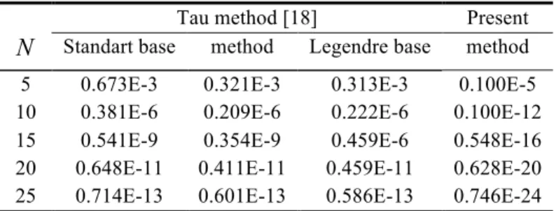
-+ = t t _dx x t x y t erf e t y 0 ) ( 1 ) ( p

which has the exact solution _y(t)=et_{. We compare the maximal errors of Tau method} and present method in Table 3.

Table 3: Comparison of maximal error of Tau method and present method N

Tau method [18] Present Standart base method Legendre base method 5 0.673E-3 0.321E-3 0.313E-3 0.100E-5 10 0.381E-6 0.209E-6 0.222E-6 0.100E-12 15 0.541E-9 0.354E-9 0.459E-6 0.548E-16 20 0.648E-11 0.411E-11 0.459E-11 0.628E-20 25 0.714E-13 0.601E-13 0.586E-13 0.746E-24

5. Conclusion

We have introduced a numerical scheme for solving systems of integro-differential equations with weakly singular kernel. The numerical scheme is based on collocation

method with using the Chebyshev polynomials whose are orthogonal polynomial bases. Some examples have been solved to illustrate the validity and efficiency of the proposed technique. The examples show that the proposed numerical scheme produces the good results and produce the desired accuracy only in a few terms with high accuracy. The method is also quite straightforward to write computer code to construct a low-cost scheme. Increasing the degree of approximation also causes the convergency of the method. These facts motivate us to state the proposed method as a fast, reliable, valid and powerful tool for solving weakly singular Volterra integral equations. The proposed method can be transformed others singular equations by using some beneficial theorems in [19].

References

[1] Frankel, J., A Galerkin solution to a regularized Cauchy singular

integro-differential equation, Quarterly of Applied Mathematics, L11 (2), 245–258, 1995.

[2] Green, C.D., Integral Equation Methods, Nelsson, New York, 1969.

[3] Hori, M., Nasser, N., Asymptotic solution of a class of strongly singular integral

equations, SIAM Journal on Applied Mathematics (SIAP), 50 (3), 716–725, 1990.

[4] Muskhelishvili, N.I., Singular Integral Equations, Noordhoff, Leiden, 1953. [5] Brunner, H., Pedas, A., Vainikko, G., Piecewise polynomial collocation

methods for linear Volterra integrodifferential equations with weakly singular kernels,

SIAM Journal on Numerical Analysis, 39, 957–982, 2001.

[6] Gülsu, M., Öztürk, Y., Numerical approach for the solution of hypersingular

integro differential equations, Applied Mathematics and Computation, 230, 701-710,

2014.

[7] Işık, O.R., Sezer, M., Güney, Z., Bernstein series solution of a class of linear

integro-differential equations with weakly singular kernel, Applied Mathematics and

Computation, 217, 7009-7020, 2011.

[8] Karimi, S., Soleymani, F., Tau approximate solution of weakly singular Volterra

integral equations, Mathematical and Computer Modelling, 57(3-4), 494-502, 2013.

[9] Koya, A.C., Erdoğan, F., On the solution of integral equations with strongly

[10] Lakestani, M., Saray, B.N., Dehghan, M., Numerical solution for the weakly singular Fredholm integro-differential equations using Legendre multiwavelets, Journal

of Computational and Applied Mathematics, 235, 3291-3303, 2011.

[11] Maleknejad, K., Arzhang, A., Numerical solution of the Fredholm singular

integro differential equation with Cauchy kernel by using Taylor-series expansion and Galerkin method, Applied Mathematics and Computation, 182, 888-897, 2006.

[12] Öztürk, Y., Gülsu, M., A collocation method for solving system of

Volterra-differential-difference equations with terms of Chebyshev polynomials, British Journal of

Applied Science & Technology, 14(4), 1-20, 2016.

[13] Parts, I., Pedas, A., Collocation approximations for weakly singular Volterra

integro-differential equations, Mathematical Modelling and Analysis, 8, 315–328, 2003.

[14] Pedas, A., Tamme E., Spline collocation method for integro-differential equations with weakly singular kernels, Journal of Computational and Applied

Mathematics, 197, 253-269, 2006.

[15] Razlighi, B.B., Soltanalizadeh, B., Numerical solution for system of singular

nonlinear Volterra integro-differential equations by Newton-Product method, Applied

Mathematics and Computation, 219, 8375-8383, 2013.

[16] Singh, V.K., Postnikov, E.B., Operational matrix approach for solution of

integro-differential equations arising in theory ofanomalous relaxation processes in vicinity of singular point, Applied Mathematical Modelling, 37, 6609-6616, 2013.

[17] Turhan, İ., Oğuz, H., Yusufoğlu, E., Chebyshev polynomial solution of the

system of Cauchy type singular integral equations of first kind, Journal of Computational

Mathematics, 90(5), 944-954, 2013.

[18] Fox, L., Parker, I.B., Chebyshev Polynomials in Numerical Analysis, Oxford University Press, London, 1968.

[19] Mason, J.C., Handscomb, D.C., Chebyshev Polynomials, Chapman and Hall/CRC, New York, 2003.