Planar p-center problem with Tchebychev distance

• ^,· .Ц X X.

7*7:· 7^ «' *щ « « ·*

PLANAR P-CENTER PROBLEM WITH

TCHEBYCHEV DISTANCE

A THESIS

SUBMITTED TO THE DEPARTMENT OF INDUSTRIAL ENGINEERING

AND THE INSTITUTE OF ENGINEERING AND SCIENCE OF BILKENT UNIVERSITY

IN PARTIAL FULFILLMENT OF THE REQUIREMENTS FOR THE DEGREE OF

MASTER OF SCIENCE

By

Dilek Yılmaz

September, 1994

I certify that I have read this thesis and that in my opinion it is fully adequate, in scope and in quality, as a thesis for the degree of Master of Science.

Assoc. Prof. Barbaros Tansel (Advisor)

I certify that I have read this thesis and that in my opinion it is fully adequate, in scope and in quality, as a thesis for the degree of Master of Science.

Assoc. Prof. O s ^ n Oğuz

I certify that I have read this thesis and that in my opinion it is fully adequate, in scope and in quality, as a thesis for the degree of Master of Science.

Prof. Akif Eyler

Approved for the Institute of Engineering and Science:

Prof. Mehme^;a3aray Director of the Institute

PLANAR P-CENTER PROBLEM WITH TCHEBYCHEV

DISTANCE

Dilek Yılmaz

M.S. in Industrial Engineering

Advisor: Assoc. Prof. Barbaros Tansel

September, 1994

The p-center problem is a model for locating p facilities to serve clients so that the distance between a farthest client and its closest facility is minimized. Emergency service facilities such as fire stations, hospitals and police stations are most of the time located in this manner. In this thesis, the planar p-center problem with Tchebychev distance is studied. The problem is known to be NP- Hard. We identify certain polynomial time solvable cases and give an efficient branching method which makes use of polynomial time methods in subproblem solutions whenever possible. In addition, a dual problem is posed in light of the existing duality theory on tree networks.

Keywords: p-Center, r-Cover, Duality

ÖZET

TCHEBYCHEV UZAKLIKLI YÜZEYEL P-MERKEZ

PROBLEMİ

Dilek Yılmaz

Endüstri Mühendisliği, Yüksek Lisans

Danışman: Doç. Barbaros Tansel

Eylül 1994

p-Merkez problemi, p tesisi talepleri karşılamak üzere en uzak talep ve ona en yakın tesis arasındaki uzaklık en küçüklenecek şekilde yerleştirme modelidir. Acil hizmet tesisleri ( itfaiye, hastane vb.) genellikle bu tarzda yerleştirilirler. Bu tez çalışmasında, Tchebychev uzaklıklı yüzeyel p-merkez problemi ele alınır. Problem NP-Zordur. Birtakım polinom çözümlü halleri belirliyor ve polinom çözümlü alt problemleri kullanan bir dallama algoritması sunuyoruz. Ayrıca, literatürdeki ağaç serimlerdeki p-merkez problemi ikil problemi çalışmalarının ışığı altında bir ikil problem öneriyoruz.

ACKNOWLEDGMENTS

I am very grateful to Associate Professor Barbaros Taiisel who has provided guidance and motivating support during this study.

I would also like to thank to my classmates Elif Görgülü, Burçin Bozkaya, Ashhan Tabanoğlu and Muhittin Demir for their friendship and patience. Finally, I would like to thank my parents, my sisters Arzu ve Aslihan Yılmaz and everybody who has in some way contributed to this study by lending moral support.

1 Introduction 2

2 Literature R eview 4

2.1 Geometry of the p-Center P r o b le m ... 6

2.2 Euclidean p -C e n te r... 9

2.3 Rectangular-Tchebychev p -C en ter... 12

2.3.1 Rectangular p-Center is N P - h a r d ... 17

2.4 D u ality ... 20

3 P roblem S tatem en t 23 4 Cover Problem Solution Approaches 26 4.1 Decomposition ... 29

4.2 Polynomially Solvable C a s e s ... 34

4.2.1 Nondominated Squares (Cliques) ... 34

4.2.2 Matching ... 38

4.2.3 Transitively Orientable Graphs ... 41

CONTENTS 1

4.2.4 Isthmus Containing Intersection G r a p h s ... 43

4.3 Local D eletion... 46

4.4 Planar Intersection G ra p h s... 48

4.5 A Solution Algorithm for the Irreducible C a s e ... 49

5 D uality 61 5.1 Cases Where the Dual Problem is Maximum Cardinality Inde­ pendent Set Id e n tific a tio n ... 64

5.2 Cases Where the Dual Problem is a Maximum Matching or a Modification of i t ... 65

5.3 A Generalized Dual P roblem ... 66

Introduction

Most of the research about the modeling and the analysis of location problems is focused on locating facilities in an optimum manner to provide services or goods to the customers who are located at given sites. The "optimum manner” is usually understood to be the minimization of the total cost (in general the transportation cost) of providing the service to the consumers. This objective allows some demand points to be too far from the facilities. However, in case of emergency service facilities such as fire stations, police stations, hospitals, it is more appropriate to mimimize the maximum cost instead of the total cost. The ”p- center problem” is a model for locating p facilities to serve clients so that the distance between a farthest client and its closest facility is minimized. Locations of radio or TV stations can also be modeled as p-center problems.

In this research, the p-center problem with Tchebychev distance is con­ sidered when the underlying location space is the plane. The problem was shown to be NP-hard by Megiddo and Supowit [18]. Our aim in the research is to identify polynomially solvable cases of the problem both in terms of the geometry of the problem and of the intersection graph obtained from the prob­ lem data. For some cases we make polynomial reductions of the problem to other solvable problems. In addition, we provide an algorithm for the resulting irreducible case that makes use of our proposed polynomial reduction tools. For the p- center problem on tree networks, the existence of duality results is due to Shier [23] and Tansel et al. [25]. Since our problem has some similar behaviour, we also explore duality for our problem.

CHAPTER 1. INTRODUCTION

The organization of the thesis is as follows:

• Chapter 2 gives a literature review about the p-center problem and the dual problem for tree networks in five sections.

• Chapter 3 gives the statement of the problem.

• Chapter 4 gives the polynomial reduction tools to solve the cover problem and a branching algorithm to solve the irreducible cases of the cover problem.

• Chapter 5 discusses duality.

• Chapter 6 concludes the thesis and discusses the contribution of our proposed algorithm and of the dual problem. Also, prospects for future work are stated.

Literature Review

Given n existing facilities in the plane, the p-center problem involves finding locations for p new facilities in a manner that minimizes the maximum distance from the closest new facility to any of the existing facilities.

Many real life problems can be modeled as a p-center problem. In fact, almost every minimax location problem with one new facility turns out to be a p- center problem when several new facilities have to be located. For instance, the problem of locating a fire station that will serve some demand points in the shortest possible time is a single facility minimax location problem. Location of several fire stations is a p- center problem.

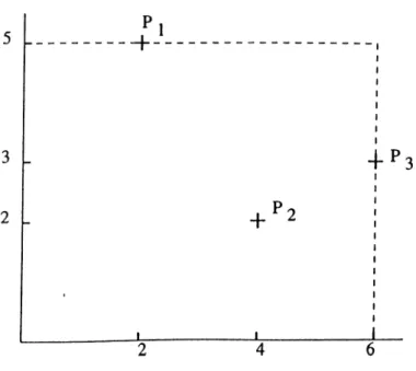
Let P = {Pi,..,Pn} denote a set of n existing facilities with Pi — (ai,bi) representing the location of the ith existing facility. Let X — {Xi , . . , Xp} denote a set of p new facilities with X j = {xj,yj) representing the location of the jth new facility. For two points Y, Z in P? with Y = (t/i,j/2)» Z = (2^1,2:2) define

d{Y,Z) = lp{Y.Z) =

(I S/l - Z, I” + I

-

;

Y)'!^

"'¡»'{I Si -

I. I -

}

if 0 < p < 00 if p = 00

Define

D{X, Pi) — min d{Xj,Pi). That is D{X,Pi) is the distance of existing Xj

CHAPTER 2. LITERATURE REVIEW

Then the formulation of the unweighted planar p-center problem is

where

/(A :)= m a x D ( X , P 0

‘ and Hp is the collection of all point sets X containing p points in it (Hp = { X : X C R \ \ X \ = p } ) .

If X* € Hp and f { X*) < f { X ) V X G Hp, we call X* a p-center and call Tp(= f{X*)) the p-radius.

An equivalent statement of the p-center problem is:

m m r s.t.

D { X , P i ) < r V P i £ P X € H p .

If each D{X,Pi) is multiplied by a nonnegative weight in the definition of f { X ) , we call the resulting problem the weighted p-center problem.

Francis [9] introduced the 1-center problem under general Ip distance. Three distances received much attention: /2, the Euclidean distance, /1, the rectilin­ ear (rectangular) distance, and , the Tchebychev distance. The p-center problem under these distance measures is proven to be NP-hard by Megiddo and Supowit [18].

The unweighted Euclidean Tcenter problem was first studied by Sylvester [24] a long time ago. Since then, there have been many studies on the Euclidean 1-center problem. Some of these studies are [7, 16, 17, 19], [22]. Megiddo [17] proposed an 0(n) algorithm using the prune-and-search method for the unweighted Euclidean 1-center problem. There is an 0{nlog^n) algorithm for the weighted Euclidean 1-center problem that combines the results in [16, 17, 19].

The unweighted rectilinear Tcenter problem can be solved in linear time by the algorithm of Elzinga and Hearn [7] and the weighted rectilinear 1-center

problem can be solved in linear time by the algorithm of Megiddo [16, 17]. For the general weighted /p-distance 1-center problem, Drezner and Wesolowsky [2] proposed an O(n^) algorithm assuming the /p-distance 1-center problem of three demand points can be solved in constant time.

For the weighted Euclidean 2-center problem, Drezner [3] proposed an O(n^) time algorithm. An ¡ogn) algorithm for the weighted Euclidean p-center problem is given by Drezner [4]. By taking into account the linear time solvability of the 1-center problem, we get a time bound of logn) for the unw'eighted Euclidean p-center problem. The Euclidean p-center prob­ lem was studied in [1, 26, 13, 14]. The best time bound is given by Hwang et al. [13], [14] as O (n ^ ).

Drezner [5] proposed three algorithms for rectilinear center problems. They are an 0(n) algorithm for the 2-center, an 0{nlogn) algorithm for the 3-center, and an 0{n?^~’^logn) algorithm for the p-center (p > 4) problem. Ko et al. [15] improved the latter problem’s time bound to 0 {‘nL’~^logn).

We will extract most important ideas from the literature after a general discussion of geometric p-center problems in Section 2.1

2.1

G eo m e try o f th e p -C en ter P rob lem

It is reasonable to start with the geometry of the simple 1-center problem. To be able to proceed further we should introduce the concept of contour sets, also called level sets, and the associated notion of contour lines or level lines . The characterizing property of a contour line is that every point on the contour line has the same value of a given function / .

We use contour lines to help us obtain insight into the shape of the graph of a function / . Each contour set, whose boundary is a contour line, is the set of all points having values of / no larger than those of the points on the contour line.

The 1-center problem is to locate a new facility with respect to n existing facilities so as to minimize the maximum distance from the new facility to the existing facilities.

CHAPTER 2. LITERATURE REVIEW

Let the location of the new facility be X = (x,y). We want to minimize the maximum distance from any of the existing facilities in P to X. That is the formulation of the 1-center problem is

min {max d(X,Pi)} xeH^ i<i<n

and an equivalent formulation is

m inr s.t.

d i X , P i ) < r , P i e P X e B ?

This problem is equivalent to the problem of enclosing n existing points in the plane within a contour set of minimum radius of the maximum distance function centered at the place where we locate the new facility. The center of the contour set, i.e. the place where we locate the new facility, is said to cover the n existing points within that radius. The problem is also equivalent to finding the minimum radius r of the contour sets centered at each existing point whose intersections is nonempty.

For the Euclidean distance measure, the contour sets are circles ( with their interiors.) If we draw a circle about each of the n points of radius r, the intersection of the n circles consists of all points whose maximum distance to the n given points is r or less. If we imagine reducing r until the intersection of the circles is a single point, we obtain the solution to the 1-center problem. An interesting insight provided by the geometry of the problem is that the minimum radius covering circle of the existing points is determined by some choice of two or three of the existing points. This is actually a result induced by Helly’s Theorem [21] which says that, in i?* , n convex sets have a nonempty intersection if and only if each fc-f 1 or fewer sets have-a nonempty intersection. Then the number of candidate r values determined by selecting three or two points from n points is -f (7^ in the plane for the Euclidean distance.

For the rectilinear case, the contour sets are diamonds, i.e. 45-degree ro­ tated squares. For the Tchebychev problem, the contour sets are squares.

Let X ' = (x', y') and let Z = (x, y) be a fixed point. The following equations show that Tchebychev contour set with radius r and centered at Z = (a:, y) is

a square:

d{Z, X' ) < r <-+ max{| x — x' \, \ y — y' \} < r

X — x' |< r and \ y — y' \< r

—r < X — x' < r and —r < y — y ' < r

<->x — r < x ' < x + r and y — r < y ' < y - \ - T

Hence the set of all points X ' whose distance from Z is at most r is a square with its center at Z and each side of length 2r.

The radius of a square is half of the side length. We draw squares of radius r about each of the existing points and then decrease r until the intersection of the squares degenerates into a line segment or a single point. The resulting intersection contains all minimax locations we sought for. The square centered at one of these minimax locations with that minimum radius r is said to be the minimum covering square of the existing points.

The following property, which we will prove later, states when the squares centered at each existing facility have a nonempty intersection.

P r o p e r ty 2.1 (P airw ise In te rs e c tio n P ro p e rty ) In the plane, k squares with sides parallel to the axes have a nonempty intersection if and only if each pairwise intersection is nonempty.O

Then, in the plane with Tchebychev distance for three squares to have a nonempty intersection it is enough for all 2 set subcollections to have a nonempty intersection and so, Helly Theorem reduces to checking all pairwise intersections to be nonempty. Now the number of candidate r values is C^.

In light of the above discussions, we can view the p-center problem as that of first determining candidate r values, then for every given r value, determining whether we can cover the existing points with p contour sets having radius r. Finding such p contour sets is equivalent to partitioning the existing points to p subsets. Actually all approaches to solve the p-center problem initiate from these observations.

CHAPTER 2. LITERATURE REVIEW

2.2

E u clid ean p -C en ter

Vijay [26] proposed a setup algorithm for reducing the number of candidate circles for a given r value from which we select p of them to cover the existing points. The algorithm depends on geometric properties of the points in the plane.

Supposing the set of existing points is partitioned arbitrarily into p sub­ sets,and the minimum covering circle for each subset is determined, the radius ' of the largest of these circles is represented by z for this partition. This largest circle is determined by two (forming a diameter) or three points (forming an acute triangle) on its circumference. The locations and sizes of the remaining p — 1 circles are not unique in general. Each circle may be moved about and varied in size arbitrarily, so long as its radius doesn’t exceed z and it still covers its subset. To reduce this degeneracy, it can be required that 1) all p circles have the same radius, 2) each circle touch at least two points if it covers two or more points, and 3)if a circle covers only one point then it is fixed at that point.

Then there are = 7i{n — 1) -f n = candidate circles with ra­ dius r or less, out of which we will choose p circles. This is done in 0(n^'’) time. Since we should make a binary search over the candidate r values the overall complexity is 0{v?^nlogn) = 0{ri^^'^^logn). This time complexity can be revised to 0{n^^~^logn) by combining it with the result that the Euclidean 1-center problem can be solved in 0( n) time.

It is advantageous to keep the number of candidate circles to a minimum. In the paper a subset of existing points that is covered by a nondominated circle is called a maximal subset and the algorithm proposed identifies dominated and redundant circles by finding all the maximal subsets for a given r value.

This setup algorithm is also extended to the rectilinear case. However, the slowest part of the entire algorithm for the cover problem is this setup algorithm.

Figure 2.1 shows a dominated circle and Figure 2.2 shows a redundant circle.

Figure 2.1. A dominates B

Figure 2.2. A or B is redundant

Chen and Handler [1] discusses a relaxation method. The authors choose a subset of the n existing points to be served and consider the circles based on one, two or three points. Using a set covering algorithm they try to find a set of p such circles which cover the points in the relaxed problem. Once they find a feasible solution (if there exists one with a maximal radius smaller than the best solution known so far) to the relaxed (reduced) problem, they check whether it is a feasible solution to the full-size problem. This is done by checking the coverage by p circles with a radius of Tp, where Vp is the largest radius of the p circles covering the reduced problem. If there is no complete

CHAPTER 2. LITERATURE REVIEW 11

coverage of the full-size problem, they add a demand point to the relaxed point, preferably the one which is farthest away from its closest service center, and solve the enlarged relaxed problem. If the solution of the relaxed problem solves the full-size problem, they have an improved feasible solution to the latter and proceed by loking for a better one. They do this by reducing to be the value of the latest feasible solution and choose again a relaxed problem and solve it. The procedure terminates when, for a given radius Tp, which is the best feasible solution known at the moment to the full-size problem, we cannot find , a solution with value less than Vp to the reduced problem. It is obvious that if no solution can be found to the reduced problem under these circumstances, there will be no solution for the full-size one. Thus the latest feasible solution to the n-points problem is necessarily the optimum. The reduced coverage problem is solved by a set-covering algorithm.

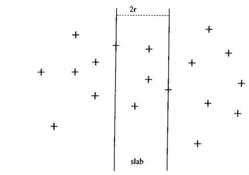
Hwang et al. [13] proposed a new technique, the slab dividing method, to solve the Euclidean p-center problem. Since the problem is NP-hard, it is not expected that the problem can be solved efficiently by the traditional divide-and-conquer method. However, the authors show that once an optimal solution of the cover problem with radius r is given, we can use part of this solution to divide the input data into two subsets Da and Dc, such that the cover problem can be solved by first solving the cover problem defined on Da and Dei respectively, and then merging the sub-solutions. Assuming that an optimal solution to the cover problem instance is given, we draw a slab with width 2r which divides the solution centers into three subsets. A dividing slab is shown in the Figure 2.3.

The authors call the solution centers in the slab as Sbi on the left of the slab as Sa and on the right of the slab as Sc- Note that the solution centers on the boundaries of this slab are assigned to

Sb-If we remove the demand points covered by Sb and divide the remaining demand points into Da and Dc, by the central line of this slab, we can see that because of the width 2r, the circles of radius centered at the solution centers in Sa (resp. Sc) cannot cover the demand points in Da (resp. Dc). This property guarantees that the two subproblem instances are independent and we call this property the independence property of the slab.

+ + + + + 2r + + + slab + + +

+

+

+

Figure 2.3. Dividing slab

than O(n^P). The algorithm stated here is also given in [14] as searching over separators strategy.

2.3

R ecta n g u la r-T ch eb y ch ev p -C en ter

It turns out that solution procedures for many location problems are more efficient for rectangular distances than Euclidean or Ip distances or network formulations.

We know that the contour line of the rectangular distance is a diamond. When we rotate a diamond by 45 degrees, we obtain a square, a result that gives a clue about the relationship between Tchebychev and rectangular distances. It

CHAPTER 2. LITERATURE REVIEW 13

is convenient to introduce the following linear transformation, which we denote by Q{x a j)·

Q{x, y) = {x + y, - x + y) = ( x\ y>)

It is direct to show that if Xi = {xi^yi) and X2 = (a^2)J/2) are two arbitrary points in the plane, then the rectilinear distance between Xi and X2 is the same as the Tchebychev distance between the transformed points Q{Xi) and Q{ X2) ; that is, h i X u X i ) = looiQ{Xi),Q{X2)) ·

It follows that the rectangular distance between any two vertices of a di­ amond D is the same as the Tchebychev distance between the corresponding vertices of the square S = Q{D) = { X : TY € D s.t.X = (^(T)}.

The consequence is that we can transform a planar location problem involv­ ing rectangular distances into an equivalent problem involving Tchebychev dis­ tances, and vice versa. Hence we obtain an equivalence between planar location problems involving Tcebychev and rectangular distances. This equivalence is useful since it is often the case that one problem is easier to analyze than the other.

After the transformation the problem is to cover the n points with p squares of equal size having the smallest possible common side length.

The transformation of rectilinear distance to Tcebychev is given in Figure 2.4.

D t m

-s

(-u;

(1,1)

r=l

(l.-l)

(-1.-1)

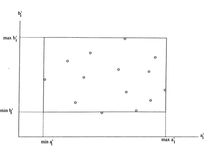
The smallest rectangle that encloses all n transformed points is called the big rectangle. An example of a big rectangle is given in Figure 2.5.

CHAPTER 2. LITERATURE REVIEW 15

b¡’

max bj

mmin

Figure 2.5. Big rectangle

Drezner [5] proposed three algorithms for the rectangular center problem. The 0{n) algorithm for the 2-center problem consists of application of two 1-center problem solution procedures. In the paper an 0{nlogn) algorithm is given for the 3-center problem. It is proved that there exists a solution to the problem where at least one of the covering squares has one of its corners on a corner of the the big rectangle. By fixing one such square with radius r the remaining problem is solved by an application of 2-center problem solution procedure. This is repeated for all the corners of the big rectangle and then for all candidate r values for the radius of the fixed square.

Drezner [5] gives an 0{n‘^^'^^logn) algorithm for the rectangular p-center {p > 3) problem similar to the Euclidean p-center (p > 3) one.

In the paper another approach yielding a lower complexity is stated. There must be a point on a side of the big rectangle. This point must be covered by one of the p squares defining the solution. One of this square’s sides must be on that side of the rectangle. Since two or three points determine a square, and one of the points is fixed, there are O(n^) such squares to be considered as part of an optimal solution. Each square covers some of the points. The remaining points define a (p — l)-center problem. The process is repeated until 3-center problems are defined. Each of these 3-center problems is solved in 0{nlogn) time. There are such problems for a total complexity of 0{'n?^~^logn).

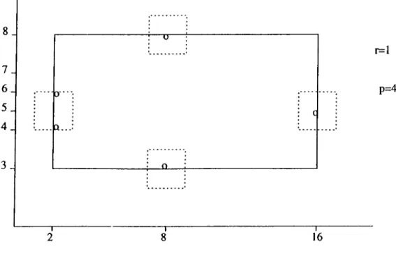
We see that for p > 3 it can’t be assured that there exist a solution to the problem where at least one of the covering squares has on of its corners on a corner of the big rectangle. The example in Figure 2.6 illustrates this.

8

Figure 2.6. No solution on the corners of tfie big rectangle

Ko et al. [15] improved the solution procedure above. It is observed that the number of squares that can cover a point on a side (left side is used in the algorithm) of the big rectangle is 0{n) for a given r. Using this idea, it

CHAPTER 2. LITERATURE REVIEW 17

is proved that there is an optimal solution to the r-cover problem such that p — 3 of the covering squares are left side squares. After placing p — 3 such squares and removing the points covered by them, the remaining problem is checking whether 3 squares with radius r cover the remaining points. This procedure is repeated for the candidate r values by binary search. Then the ovei'all complexity becomes .0{n).0{logn) = 0 { ‘nL’~^logn).

2.3.1

R ecta n g u la r p -C en ter is N P -h ard

Megiddo and Supowit [18] proves the NP-hardness of the p-center problem by showing the NP-completeness of the related decision problem, the cover problem. Then the question is: Given n unit squares in the plane, with sides parallel to the axes and an integer p > 0, are there p points such that each square contains at least one point?

To prove that the square covering is NP-complete we should show that 1) the square covering € NP and 2) a known NP-complete problem can be polynomially transformable to the square covering.

1) holds since given p points, there exists a Nondeterministic Turing Ma­ chine that checks polynomially whether each square contains at least one of these points.

To show that 2) holds, 3-SAT is transformed to the square covering.

Formally, given a boolean expression E = E\ A E2 A ... A Em, where Ej = Xj V Vj V Zj ( {xj,yj,Zj} Ç {«i,üi,U2,t/2, ...,u „ ü ,} ), the 3-SAT problem is to decide whether there exists a set S Ç {xj,yj,Zj} Ç {ui,üi,U2>W2,

such that

S n {xj,yj,Zj} / 0 , (; = l,2 ,..,m ),

and

I S n {u,-,u,·} 1= 1 , (i = 1,2, ..,9 ).

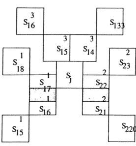
The transformation from 3-SAT to the cover problem will be established as follows. First, variable u, is represented by a circuit S'},.., S'rJ, of squares

as is shown in Figure 2.7; r, is even.

A circuit in the reduction for square covering.

Figure 2.7. A circuit

Two squares of a circuit intersect if and only if they are adjacent. A clause configuration is shown in Figure 2.8.

Each clause E, is represented by a single square Sj that touches the three circuits involved. A junction is illustrated in Figure 2.9.

In a junction we simply coalesce a square of one circuit with a square of the other circuit. The coalesced squares must each be odd indexed in its respective circuit so that there will be an odd number of squares between consecutive junctions of a circuit. The four corners of the junction square correspond to the four combinations of possible truth values for the corresponding variables.

CHAPTER 2. LITERATURE REVIEW 19

A clause configuration in the reduction for square covering.

Figure 2.8. A clause configuration

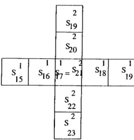
Thus, in order to cover all the circuits, we need p = X^r,/2 — J points, where J is the number of junctions. If E is satisfiable then p points suffice for covering the clause configuratios as well as the circuits if the type of cover in each circuit is chosen appropriately. Conversely, suppose that p points suf­ fice to cover the entire structure. Then consider segments of circuits between consecutive junctions: ■ · , where Sj^ and S'/ are consecutive junction squares in the circuit for u,. We need I^ r,/2 — 2J points in order to cover all these segments. We are therefore left with only J more points with which to cover the junctions and the clause configurations. It follows that the cover by p points induces truth values that satisfy E. This completes the proof that 3-SAT is transformable to the square covering. The reduction is polynomial. Therefore the square covering is NP-complete and the related optimization problem is NP-hard.

2 Si 9 2 ^ 0 1 s 15 1 ^16 1 2 1 ^18 1 s 19 2 S 2 2 2 S 2 3

A junction in the reduction for square covering.

Figure 2.9. A junction

2.4

D u a lity

For the p-center problem when the location space is a tree network or R^ a new location problem "dual” to the original problem has been identified. The question arises if some of these duality results can be extended to the planar case, at least for the case of /i or l^o metric.

One such result is presented by Shier [23]. The primal problem is to locate p centers on a tree network in order to minimize the maximum distance from an}' point on the tree network to its nearest center (continuous p-center).

In the paper an equivalence between (a) finding the smallest radius r possi­ ble for p covering neighbourhoods and (b) finding p-f-1 points that are ”as far apart as possible” in the sense of having their minimum separation as large as

CHAPTER 2. LITERATURE REVIEW 21

possible, is identified. There is thus determined a distinct but related maximin location problem which is ”dual” to the original minimax p-center problem.

Namely, the dual problem is to place a fixed number of points on a network which are as far apart as possible from one another. This latter problem of locating "mutually obnoxious” facilities could arise in the placement of strate­ gic resources (e.g., oil refineries, ammunition stockpiles) so that accidents or interventions at one facility will not endanger other facilities. In order to demonstrate the validity of the above duality statement, the author makes use of another minrnax result which deal with covering a tree T with neighbour­ hoods of a fixed radius r > 0. The assertion is that the minimum number of neighbourhoods of radius r needed to cover equals the maximum number of points of T which are mutually separated by a distance exceeding 2r.

Another duality result is presented by Tansel et al. [25]. The problem con­ sidered is a nonlinear p-center problem on a tree network in the presence of distance constraints. The centers provide a service to demand points located at vertices of the network, and the "cost” of providing service to a given de­ mand point is expressed as a strictly increasing and continuous "loss” function whose argument is the distance between the demand point and a closest center. The constraints on center locations specify a nonnegative upper bound on the distance between aech existing facility and its nearest center. Related covering problem is to locate the minimum number of centers such that the loss function value of each demand point does not exceed the parameter r.

In the paper the dual of the p-center problem which is called the dual threat problem and the dual of the related cover problem which is called the dual divergence problem are identified. For each pair of problems, weak and strong duality results are given. It is proven that the minimum r value by which p centers cover the demand points located at the vertices of the network is equal to the maximum value of the minimum pairwise covering cost between the choosen p -f 1 vertices (dual threat). It is also proven that the minimum number of facilities to locate to cover the demand points within a cost of r value is equal to the maximum number of demand points no two of which can be covered together by a facility within a cost of r value (dual divergence).

All of the four problems stated above are solved using variants of a covering algorithm called COVER, which is an 0{n) algorithm. That is, the covering

algorithm provides the basis of the solution procedure to the dual problem (as well as the p-center problem) and yields a constructive approach for proving strong duality (equal primal and dual objective values at optimality of each problem) results. An O(n^) version of COVER is used to prove these results.

C h a p te r 3

Problem Statement

We will deal with the planar unweighted p-center problem and the related cover problem with loo, Tchebychev metric. That is, we take d{Xj,Pi) = loo{Xj,Pi) for j = 1, ..,p ; f = 1, ..,n , and seek for a solution (rp, X*) to the problem

rp = f i x * ) = mm f { X) = max mm d{Xj, P )

where Hp = { X : X C | X j= p}. We call X* a p-center and call rp a p-radius.

An equivalent statement of the p-center problem is:

min r s.t.

D { X , P i ) < r W P i e P x e H p

where D{X, Pi) = min diXj,Pi). Xj^X

Assume now we have found an optimal solution to the p(p > 2)-center problem. Then we can partition the existing points by assigning each existing point to its closest center. If there are points that are covered by more than one center, then we assign each such point to one of the centers arbitrarily. Now,we know from the single facility minimax theory that each resulting disjoint subset of existing points can be optimally covered by a minimum covering square. We also deduce from the single facility minimax theory that two existing points

that are maximally separated in a disjoint subset determine the radius of the minimum covering square. This gives p critical squares the largest of which has a radius Tp. Then we conclude that among all optimal solutions to the center problem of serving n existing points in the plane there is one which is determined by critical squares the largest of which has a radius Vp which is the optimal solution value. Then the number of candidate values for r is pairwise distances among the existing points.

To solve the p-center problem we will make a binary search over the can­ didate r values and for a chosen one we will ask: are there p squares having radius r which cover the given existing points? This last problem for a given r is called the r-cover problem. To give a precise formulation, let / = {1, ..,n ) be the index set corresponding to the existing points and let i'i? = : i e 1} be a family of squares having radius r and centered at each P,. The r-cover problem is finding a point set X = { ^ i, ··■, Xq} with each X j € so that | X | is minimum and every Si has a point in common with X (that is , every P,· is covered by some X \j^ within a distance of r).

(CP) I X* 1= m in I X I s.t.

X n 5 . · € I

X

c

Here each X j corresponds to the center of the minimum covering square with radius r.

The cover problem is equivalent to the partition problem which asks: can we partition the index set / = { l,..,n } of the existing points into smallest number of subsets, say, / i , .., / „ in such a way that n.e/^ P, ^ 0 for j = 1,.., q. Let P be a partition of I. That is P = { / i ,.., R} for some integer t {I < t < n ) such that each index i in I belongs to one and only one of the subsets / i , .., p and / = Denote by H the class of all partitions of I. The partitioning problem is as follows:

Find a partition P* in H such that

(PP) I P* 1= m in I P I s.t.

CHAPTER 3. PROBLEM STATEMENT 25

Oiei, Si + 0,V/,· e P P e n .

P r o p e r ty 3.1 PP and CP are equivalent.

proof: Suppose P* solves PP. Let P* = Since fl.g/j Si ^ 0 for j = 1, let Xj be a point in D.g/^ Si. Then X = { X i,.., X J is feasible to CP. Furthermore, X is optimal to CP as otherwise there exists some Q = {qi, .., q^} with s < t such that Q f] Si ^ 9 for all i e I. Let J\ be the set of indices j in I for which qi 6 Sj. Then define J2 to be the set of indices j in / — Ji for which q2 € Sj. Continue this process so that, finally, Js is the set of indices j in 7 — Ufri J, for which qs € Sj. Then P = { J i ,.., J«} is feasible to PP as <lj € n,6/j Si and so | P |< | P* |, contradicting the optimality of P*.

Suppose now X* solves CP. Then a similar procedure to the one in above paragraph will determine a partition P which is feasible and optimal to PP, with I p 1=1 p* !.□

Cover Problem Solution Approaches

We will concentrate on the r-cover problem,

(CP) I X* 1= min I X I s.t.

X f\ Si ^ ^ I X

c

to solve the p-center problem.

Here each X j corresponds to the center of the a minimum covering square with radius r. We will represent the cardinality of X* as q{r : P) or as q{r : I) where P = { P i , P n } is the set of existing points and I is their index set. In addition, for any subset P of I we let q{r : I') = min{| X \: X 0 Si / 0,i € r ,a n d X c R '^ }

If I X* 1= q is less than or equal to p, then we try a smaller r value in the candidate list {(l/2)/co(P,·, Pj) : 1 < * < i < >i}· If not, we try a greater r value. We stop at an r value for which q{r : P) < p while q{f : P) > p where f is the largest value in the candidate list that is less than r.

It is straight forward to show that Vp > Vp^i for p = 1,2, . . , p — 1. Since we solve the p-center problem by solving a series of cover problems over the candidate r values, we may drop the candidate r values greater than or equal to T3 by applying Drezner’s 3-center 0{nlogn) algorithm.

CHAPTER 4. COVER PROBLEM SOLUTION APPROACHES 27

As mentioned earlier, the cover problem is equivalent to the partition prob­ lem which asks for a partition of the index set I = {1, ..,n} into the smallest number of subsets, say, 7 i , /,, such that 0,^/^ 5, ^ 0 for j = 1, ..,q .

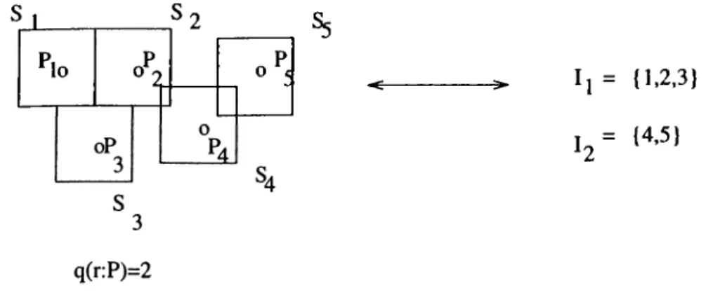
In Figure 4.1, there is an r-cover such that the points Pi, P2 and P3 are covered together while P4 and P5 are covered together within r distance. This is equivalent to stating that there is a minimum cardinality partition of these points’ indices into {1,2, .3} and {4,5} such that, for each subset, the corre­ sponding squares have a nonempty intersection.

> 1 ‘^2

Plo o'; _{I l = {1.2.3}}

H.5I

Figure 4.1. Cover is equivalent to partition

P airw ise In te rse c tio n P ro p e rty (Property 2.1) In the plane, k squares with sides parallel to the axes have a nonempty intersection if and only if each pairwise intersection is nonempty.

proof:

Let SQi, i = l ,..,k be k squares in with sides parallel to the axes. Without loss of generality let (a,·, A) be the center and r,· be the radius of SQi . Let L] = [a, - r,,Ofi -f r,] be the x axis projection of SQi and L] = [yj. _ r·^ ^i + ri] be the y axis projection oi SQi for e = Let LL = L ]f\L j and Lfj = Li] for I < i < j < k. We should prove that 0 iff SQi

n

3(x,j/) € R"^s.t. max{| x - a,· |, 11/ - < r,· Vi iff

3{x,y) € R^ s.t. I X — a,· |< r,· Vi and | y — /?,■ |< r,· Vi iff

njLjL,· ^ 0 and nf_jL? ^ 0 iff from Helly Theorem,

L] n Tj ^ 0, 1 < f < i < and I? n TJ 0, 1 < i < ;· < iff X L?. / 0 1 < i < i < A: iif

SQi n SQ j 7^ 0 1 < i i

Let G = be the intersection graph with node set / and the arc set A consisting of undirected arcs (¿,y) for every pair i , j E. I , i ^ j for which SiOSj 7^ 0. Note that the arc set depends on the value of r and is nondecreasing with increasing r.

When G is formed in this way, a clique in G is a complete subgraph of G (i.e. every pair of nodes in this subgraph is connected by an arc in A). Since {i,j) 6 A iff 5; n Sj 7^ 0, the node set of a clique defines a subcollection I' of / such that n,g/' S{ 7^ 0.

Then, we may view the r-cover problem as an equivalent clique cover prob­ lem on the intersection graph. Finding a minimum cardinality clique cover identifies node sets /1, R such that each node set forms a maximal clique. It is clear that solves the partition problem and that q{r : I) = q{r : h ) + ·· + ? ( ’' ·’ h)· Thus, by solving an r-cover problem for each node set 7j, we have a solution to the r-cover problem (on I) by taking the union subproblem solutions.

CHAPTER 4. COVER PR0BLEA4 SOLUTION APPROACHES 29

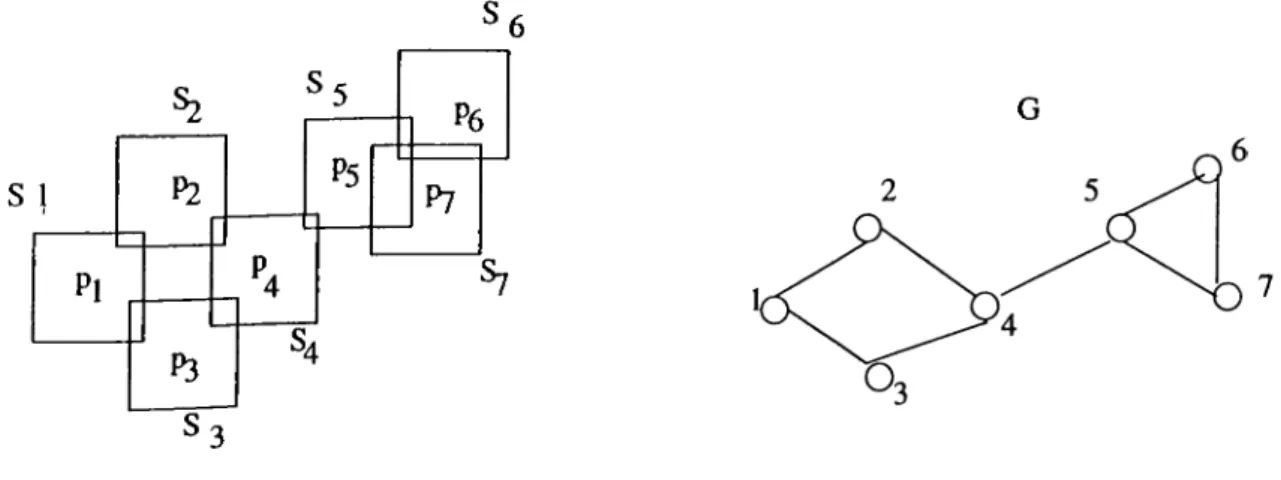
For example, when we have n — 1 with 2r = 2 a planar data and its intersection graph are given in Figure 4.2.

S 1 Pi P2 P3 P5 P6 P7 G

Figure 4.2. A planar data and its intersection graph

We will make use of both the geometry of the problem and the correspond­ ing intersection graph interchangeably.

4.1

D e c o m p o sitio n

Pj = {aj,bj) and Pk = (ak,bk) {I < j < k < n) can be jointly covered by a single point within a distance of r if and only if d{Pj,Pk) < 2r.

The necessity part is trivial. Sufficiency follows directly from Property 2.1 ( Pairwise Intersection Property) when the squares under consideration are the two squares centered at Pj, Pk each having radius r.

Then Pj and Pk {I < j < k < n ) are coverable by one Xi within r distance units iff their x-coordinate and y-coordinate separations are both less than or equal to 2r. If in at least one coordinate their separation is more than 2r the points can’t be covered together. By making use of this conclusion we can decompose an r-cover problem into smaller problems whenever possible.

Let’s assume that all existing points lie in the first quadrant of R? without loss of generality. We project the existing points to the x and y axes and draw a vertical line (strictly) between two adjacent points on the x-axis if they are more than 2r distant from each other and a horizontal line (strictly) between two adjacent points on the y-axis if they are more than 2r distant from each other . These vertical and horizontal lines divide the big rectangle into smaller rectangles which we refer to as boxes. We will call the the region between two vertical lines a vertical block and between two horizontal lines a horizontal block.

P ro p e rty 4.1 No two points from different boxes can be covered together.

proof:

Let B\ and B2 be two of the boxes obtained. We observe that one of the following three is true: 1) Bi and B2 are in the same vertical block but not in the same horizontal block, 2) Bi and B2 are in the same horizontal block but not in the same vertical block, 3) B\ and B2 are neither in the same vertical block nor in the same horizontal block.

For case 1), the closest points from Bi and B2 are separated by more than 2r in the y-axis.

For case 2), the closest points from Bi and B2 are separated by more than 2r in the x-axis.

For case 3) the closest points from the two boxes are more than 2r distance away from each other in both axes. Hence, no two points, one from Bi , the other from B2 , can be jointly covered by one point. □

The decompositon procedure stated above is 0{n).

Due to the above property we decompose the data into smaller parts and solve them independently.

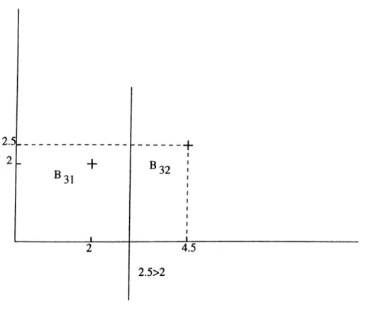
Figure 4.3 gives an example on a 4 point r = 1 cover problem where the data is decomposed first into three subproblems where the corresponding data lies in 5 i, B2 and B3

CHAPTER 4. COVER PROBLEM SOLUTION APPROACHES 31

We can further decompose B3 and then solve B i, B2, B31, B32 and B4

Figure 4.4. Further decomposition

When we look at what this decomposition means in terms of the correspond­ ing intersection graph, we see that the decomposition procedure produces boxes such that intersection graph of the nodes in each box is a number of components of the original problem. This means that not every component of G = (/, A) may be accounted for by the decomposition. Figure 4.5 demonstrates a case where decomposition doesn’t apply while G consists of two components.

CHAPTER 4. COVER PROBLEM SOLUTION APPROACHES 33

O

O'

Figure 4.5. A nondecomposable case

Let G' = (/', A') be the intersection graph of a nondecomposable box that encloses points P, , i € I'. To determine all the components of this intersection graph we do the following. Define Ii = and I\ = I — I\. Find neighbours of h in I\. Add these neighbours to I\ and delete them from ly. Continue adding neighbours from ly into ly until no more neighbours can be added. The final ly defines the node set of a component of G' that contains i. This process finds one such component in O(n^) time, finding all components require O(n^) time.

We identified some polynomially solvable cases by examining the geometry of the problem data and the corresponding intersection graph and obtaining some nondomination results.

4.2

P o ly n o m ia lly Solvable C ases

4.2.1

N o n d om in ated Squares (C liques)

We are trying to find a minimum cardinality set X = where the squares of radius r centered at those points, Sx^ , j = cover the demand points We claim that when certain conditions are satisfied we can identify some nondominated squares; that is by covering some of the points by these squares we don’t lose optimality.

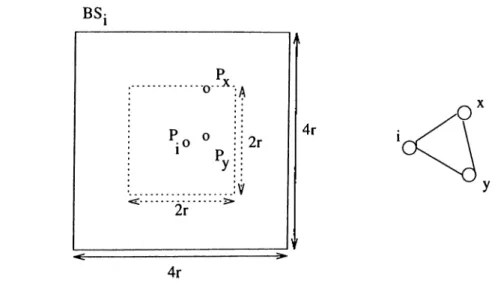
Union of all squares that can cover P, within a radius r is just a square of radius 2r centered at P,. We will call this square cis the big square of P, and represent it as BSi. The following figure shows the big square BSi

BS;

Figure 4.6. Big square

Let’s draw the smallest enclosing rectangle of the points in the big square B Si. If it is a rectangle whose longer side is at most 2r, then we take a square of radius r containing this rectangle and call it a nondominated square. In terms of the intersection graph, we are trying to find a node i such that all the nodes adjacent to it form a maximal clique together with i and we call that clique a nondominated clique. A nondominated square determined by P, and all of the points in its big square and the corresponding nondominated clique

CHAPTER 4. CO VER PROBLEM SOL UTION APPRO A CHES 35

is given in Figure 4.7.

4r

Figure 4.7. Nondominated square(clique)

P r o p e r ty 4.2 In the intersection graph G—(I,A), if there is a node v such that

V and all o f the nodes adjacent to it form a clique, then there is a minimum

clique cover of I where the clique formed by v and its adjacent nodes is one of the cliques.

proof: Let K = {G i,..,G ,} be a minimum clique cover of the node set with Gi = (K i,A i), i = That is, each Gi is a complete subgraph with node set Ki where Ki fl Kj = 0,i j , while U;_i K; — I. Note that Q A.

Since U’_i Ki = I, V belongs to some Ki ; say Ki w.l.o.g. Let Ni be the set of nodes in I that are adjacent to v. Either Ki = A^i U{u} or not. In the former case the assertion is true. In the remaining case coastruct a new clique cover K ' from K as follows: Replace Ki by K[ = N \O K i and cover I —K[ minimally. Since iVi includes all neighbouring nodes of v and Ni U {u} forms a clique by assumption, we have Ki C N iU K\. This implies K ' = A^i U K\ = N iO {u}. Put q{P) = q{r : V) for any subset V of I. Then,

g(I) = q = ^ + q ( / - K i )

cliqueKj

=> q{I — K \) q — I and

\ K '\ = ^ +q{I - [N ,\J K ,)).

cliqueK[

Since ( / — (A^i U Ki )) C ( / — Ki ), we have

q { I - { N , O l U ) ) < q { I - I u )

^ q { I - { N , O K , ) ) < q - \

=>| K' 1= 1 + q{I - (A'l U /fi)) < 1 + g— 1 = 7

M K ' \ < q

Since q is the cardinality of a minimum clique cover we don’t lose optimality by covering / by K' .□

This nondominated clique identification is of order O(n^), since maximum n nodes are checked each requiring checking at most n adjacent nodes.

By application of nondominated clique identification process we reduce the size of the remaining problem and in some cases solve the whole problem.

CHAPTER 4. COVER PROBLEM SOLUTION APPROACHES 37

Figure 4.8. Case solvable by nondominated cliques

In cases where the big rectangle’s smallest side length is less or equal to 2r, r-cover problem can be solved by nondominated square identification. The reason is that a point on one of the smallest sides of the rectangle defines a nondominated square and the removal of the points covered by that square leads to other nondominated squares.

A generalization of this case is given in Figure 4.9, where the existing points lie in rectangles having the smallest side length less or equal to 2r such that the closest points from different rectangles are more than 2r distance apart. In such a case, r cover problem can be solved by identifying nondominated squares for each rectangle separately.

2r

2r

-e--- >· 2r

A case solvable by left-right or

up-down nondominated square identification

Figure 4.9. Case solvable by nondominated squares

4.2.2

M atch in g

In graphs where there are no 3-cliques, maximum matching gives a lower bound to the minimum clique cover problem. We will state when maximum matching and minimum clique cover give the same solution in these graphs and also state how we form a modification of a maximum matching to obtain a minimum clique cover.

P ro p e rty 4.3 Let G be an intersection graph containing n nodes where there are no 3-cliques. The maximum matching cardinality is at most n /2 , since each matched edge corresponds to two nodes and the matched edges share no nodes. I f maximum matching cardinality is n/2 , then minimum clique cover is obtained by that maximum matching. Else if the maximum matching cardinality k is such that n/2 > k , then minimum clique cover cardinality is n — k and minimum clique cover is composed of k matched pairs and n — 2k singletons.

CHAPTER 4. COVER PROBLEM SOL UTION APPRO A CHES 39

proof:The assumptions imply that the maximum clique size in these graphs is 2. When the maximum matching cardinality is n/2 ,it exhausts all n nodes and since the maximum matching cardinality is a lower bound on the cardinality of a minimum clique cover in these graphs we can’t do better than this lower bound. Therefore, maximum matching gives a minimal clique cover in that case.

Let’s consider the case when all nodes are not exhausted by a maximum matching, i.e. there are unmatched nodes. Since the maximum clique size is 2 we can’t achieve a better solution to the clique cover problem than the solution determined by k 2-cliques of a maximum matching and n — 2k 1- cliques corresponding to the unmatched nodes. □

In Figure 4.10, a graph satisfying the assumptions of the above theorem is given where all nodes are exhausted by a maximum matching which also solves the minimum clique cover problem. In the same figure, another graph which has no 3-cliques is given where the maximum matching cardinality is 7 and this is the maximum number of 2-cliques. The best we can do to solve the minimum clique cover problem is to cover the matched nodes pairwise and the unmatched nodes by themselves.

max matching gives min clique cover

k=7 and min cover is 16-7=9

Figure 4.10. Matching or modification of it solves the cover problem

We should note that maximum matching is solved in O(n^) time [20].

We can solve some cover problems first applying a series of clique reductions in the intersection graph and then if the remaining graph conforms to the assumptions above we solve a maximum matching. Figure 4.11 shows such a solution.

CHAPTER 4. COVER PROBLEM SOLUTION APPROACHES 41

clique reduction + matching

Figure 4.11. Nondominated cliques and then matching solves the cover problem

4 .2 .3

T ran sitively O rientable G raphs

Let G=(I,A) be a graph. We will represent a directed arc from a node i to a node j as ij where i and j are elements of I. G is transitively orientable if there exists an orientation (I,F) of G obtained by assigning a one-way direction to each edge such that ab Ç; F A be € F => ac £ F,Va,b,c e I. Such an orientation (I,F) is called a transitive orientation. Here, every directed path in F corresponds to a clique of G because of transitivity. A node which has no incoming arcs in F is called a source of F and a node which has no outgoing arcs in F is called a sink of F\

Transitively orientable graph recognition and finding a transitive orienta­ tion can be done in polynomial time, 0 (6 | A |), where 6 is the maximum degree of a node in the graph G (Golumbic [10]).

Golumbic [10] transforms a transitive orientation (I,F) of G into a trans­ portation network by adding two new nodes s and t and arcs sx and yt for each source X (a node that has only outgoing arcs) and sink y (a node that hcis only

incoming arcs) of F. Assigning a lower capacity of 1 to each node, they ini­ tialize a feasible integer-valued flow and then call a minimum-flow algorithm. The flow’ s feasibility implies that every node is covered. The algorithm will try to use minimum number of directed paths to minimize total flow sent and since each directed path corresponds to a clique, the number of cliques used will be minimized. Then the value of the minimum flow will equal the size of the minimum covering of the nodes by cliques. Minimum flow problem is solvable in 0{n^) time.

Figure 4.12 shows two transitively orientable graphs with their orientations. In the figure on the left, the minimum flow value is 2 and this is the same as the minimum clique cover cardinality. In the other figure, the minimum flow value is 3 so the minimum clique cover cardinality is 3.

2 P

• o s

Ô

CHAPTER 4. COVER PROBLEM SOLUTION APPROACHES 43

4 .2 .4

Isth m u s C ontainin g In tersectio n G raphs

An isthmus in a graph is an arc whose deletion increases the number of com­ ponents.

P r o p e r ty 4.4 Let G be a graph. Assume that there exists an isthmus con­ necting nodes v\ and V2, w.l.o.g. Let Si , S2 be the two disconnected subgraphs . resulting from the deletion of arc (^1,^2) with Si containing vi and S2 con­

taining V2- I f S i ’s minimum clique cover cardinality remains the same in a minimum clique cover of the subgraph obtained by adding V2 and (01,02) to Si, we can cover G minimally by covering vi and 02 together.

proof:

Let the cardinality of a minimum clique cover of Si be q and of S2 be s. Denote the subgraph obtained by adding 02 and (ui,t»2) to Si as and the subgraph obtained by deleting the node 02 and incident arcs to it from S2 as S'2. Let the cardinality of a minimum clique cover of S[ be q' and S'2 be s'.

From the assumptions we know that q = q'. To have that after addition of

02 to Si, there should be a minimum clique cover of in which vi and 02 are in the same clique since 02 is incident to only vi.

Since there are more nodes in S2 than S'2, s > s'. Then ^-|-s = > q'+s'. This means that we don’t lose optimality by covering Oi and 02 together. □

Figure 4.13 shows a case where the isthmus forming nodes are covered together.

P r o p e r ty 4.5 Let G be a graph. Assume that there exists an isthmus connect­ ing nodes Oi and 02 , w.l.o.g. Let Si denote the subgraph containing Vi and S2

denote the subgraph containing i>2· I f Si ’s minimum clique cover cardinality increases in a minimum clique cover of the subgraph obtained by adding 02 and (01,02) to S i, we can cover G minimally by covering vi and 02 separately.

Let the cardinality of a minimum clique cover of Si be q and S2 be s. Denote the subgraph obtained by adding V2 and (ui,U2) to Si as S[ and the subgraph obtained by deleting the node V2 and incident arcs to it from S2 as S'2. Let the cardinality of a minimum clique cover of ¿"i be q' and S'2 be s'.

From the assumptions we know that S 'l’s minimum clique cover cardinality increases with the required additions and this increase can’t be greater than 1 , since only a single node is extra and so qf' = 9 + 1. Since there are one less nodes in S'2 than S2, s' = s or s' = s — 1 .

Then either 9' + s' = i ' + s = <j' + l + s > ^ + s o r g ' + s' = ^' + s — 1 = + s — 1 = q + s. That is, + s' > 9 + s meaning we can cover G minimally by minimally covering Si and S2 separately. □

Figure 4.14 shows a case where the isthmus forming nodes are covered separately.

CHAPTER 4. COVER PROBLEM SOLUTION APPROACHES 45

Figure 4.14. The nodes forming isthmus are covered separately

To identify the existence of an isthmus, we delete an arc (ui,U2) and then solve a shortest path problem to determine whether there is any path between the nodes Vi and V2 after deletion. We repeat this procedure for each arc in the intersection graph. The time bound of these operations is 0{\ A \ n^).

We can solve minimum clique cover problems in some intersection graphs using our polynomial tools. For example, in Figure 4.15, two nondominated cliques are identified first. After the removal of the nodes covered by these cliques, what results is a graph where there is an isthmus making it possible to solve the components separately. One of the components is solved by m atch­ ing and the other component is a transitively orientable one that is solvable polynomially, too.

Figure 4.15. A polynomially solvable case

4.3

Local D e le tio n

The solution value of the modified problem resulting after deletion of a point gives a lower bound to the minimum cover solution value of the original prob­ lem.

However, there exist cases where there is no gap between the lower bound and the optimal value.

Figure 4.16 shows a case where local deletion gives a strict lower bound to the value of the r-cover problem for the original data.

CHAPTER 4. COVER PROBLEM SOLUTION APPROACHES ₄₇

min cover=3 min cover=2

Figure 4.16. Local deletion: gap between lower bound and optimal value

What are the properties of Pi whose deletion doesn’t cause a reduction in the optimal value?

P r o p e r ty 4.6 Assume that there is an optimal solution for the modified prob­ lem that results after the deletion of a point Pi such that there exists nondom- inated squares with radius r, N Si, i — l,..,s . Let the set of points covered by N Si be Qi i = l,..,s . If at least one set Qi i = l ,..,s is a subset of the points in the big square of Pi in the original pi'oblem, then P i ’s removal doesn’t create a gap.

proof: Let Qi be a set which is a subset of the points in the big square of Pi. It follows that all points in Qi are within 2r distance of Pi. Since Qi is the set of points covered by a nondominated square, all points in Qi are within 2r distance of each other. Therefore Pi and the points in Qi are within 2r distance of each other and they can be covered by a single center X i within r distance. Let be a square with radius r centered X i. After deletion of Pi, N S i defines a nondominated square for the modified r-cover problem by construction. Since the solution obtained to the modified problem gives a lower bound and by construction cover Pi, there is no gap between the cardinalities of the r-cover problems. □

We see that in Figure 4.17, deletion of the point Pi creates no gap since there is a minimum cover of the resulting problem where P4 defines a nondorninated square and it can be covered with Pi.

In some cases, after deletion of one or more points whose deletion does not create optimality gap, the resulting problem is polynomially solvable. To identify such a point we delete a point and look for a nondominated square formed by only points from the big square of the deleted point. This is done with a time bound of O(n^) for a point.

P6 P5 ^7 Ps Pi ^2 P4 P3 P 6 P P P 5 7 8 q(r; P)=4 q(r: P-{P j })=4

Figure 4.17. Local deletion: no gap

4.4

P lan ar In tersectio n Graphs

A graph is planar if it can be drawn on the plane (or on the surface of a sphere) such that no two arcs cross one another. Equivalently, a graph G is planar iff there is no subgraph of G ( consisting of a subset of nodes of G and of arcs that connect only these nodes ) homeomorphic to A'5 or .