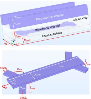
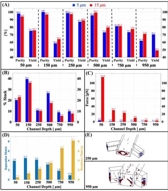
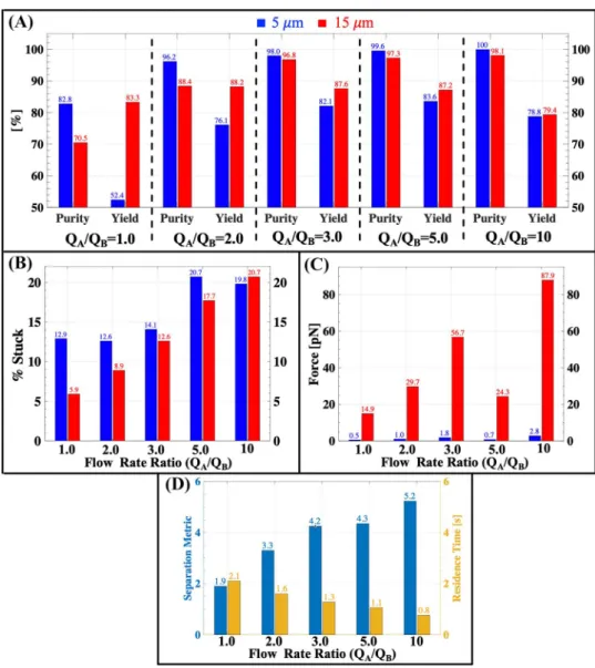
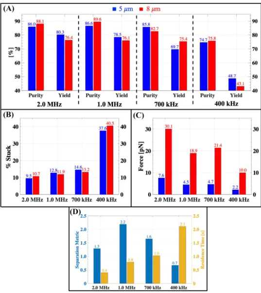
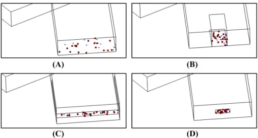
Investigation of effect of design and operating parameters on acoustophoretic particle separation via 3D device-level simulations

These feasibility con- ditions are related with : arrival time of a path to destination node because of the scheduled arrival time to destination node; arrival times to

Apergis and Payne ( 2009 ) examined the relationship between economic growth and energy consump- tion in 11 countries within Commonwealth of Independent States, and found that a

Bu araştırmanın bulguları yeterli alan bilgisine sahip öğretmenlerin hem teknoloji bilgisini hem de pedagoji bilgisini bu alan bilgisine entegre etmeye özgüvenlerinin

studies, deregulation, domestic asset markets, financial liberalization, financial rents, Fiscal Gap, income, Income Distribution, income inequality, inequality, integration

^ Variables are: 1) commercial bank debt; 2) concessional debt; 3) variable-rate debt; 4) short-term debt; 5) FDI; 6) public sector debt; 7) multilateral debt; 8) the ratio

Keywords: Reengineering, Operations Improvement, Manufacturing Productivity, Factory, Assembly, Machining, Material Handling, Changeover/Setup, Focused Factory,

Brockelman‘ın Ġslâm Milletleri ve Devletleri Tarihi adlı eserinde Abbasi halifelerinden Halife Mansûr, Mehdî, Harun er-ReĢid ve Abbasilerin ilim ve ilâhiyat

Çalışmamızın birinci bölümünde, 2000-2016 arası dönemde dünya ekonomisinde büyüme, dış ticaret kolları olan ithalat ve ihracatın durumu enflasyon ve