Replenishment and transportation pricing decisions under two independent carriers with different modes

(1)

REPLENISHMENT AND TRANSPORTATION PRICING

DECISIONS UNDER TWO INDEPENDENT CARRIERS WITH

DIFFERENT MODES

A THESIS

SUBMITTED TO THE DEPARTMENT OF INDUSTRIAL ENGINEERING

AND THE INSTITUTE OF ENGINEERING AND SCIENCE

OF BILKENT UNIVERSITY

IN PARTIAL FULFILLMENT OF THE REQUIREMENTS

FOR THE DEGREE OF

MASTER OF SCIENCE

By

Safa Onur Bingöl January, 2009

(2)

I certify that I have read this thesis and that in my opinion it is full adequate, in scope and in quality, as a dissertation for the degree of Master of Science.

___________________________________ Assist. Prof. Dr. Ayşegül Toptal (Advisor)

______________________________________ Assist. Prof. Dr. Alper Şen

______________________________________ Assist. Prof. Dr. Nagihan Çömez

Approved for the Institute of Engineering and Science

____________________________________ Prof. Dr. Mehmet Baray

(3)

ABSTRACT

REPLENISHMENT AND TRANSPORTATION PRICING DECISIONS

UNDER TWO INDEPENDENT CARRIERS WITH DIFFERENT MODES

Safa Onur Bingöl M.S. in Industrial Engineering

Supervisor: Assist. Prof. Dr. Ayşegül Toptal January, 2009

Freight transportation constitutes a substantial cost component in global economics and consumes significant amounts of energy. With the increasing oil prices, scarcity of resources and environmental concerns, efficient operation of transportation activities has become even more important than it was in the past. These raising concerns necessitate the companies which utilize this activity to plan for transportation more carefully and conservatively, and the ones that support it to appraise its value more cautiously.

In this thesis, we consider a setting consisting of a retailer, a truck-load carrier and a less-than-truck-load carrier. We model and solve the retailer’s integrated inventory and transportation problem under the presence of two modes of carriers. Characterising the solution for the retailer’s replenishment problem, we then analyze the transportation pricing decisions of the carriers. We show that substantial savings can be achieved by the retailer due to integrating inventory and transportation decisions. We also quantify the savings for the TL carrier and the LTL carrier through carefully determining their transportation price schedules.

Keywords: Transportation pricing, Truckload carrier, Less-than-truckload carrier,

(4)

ÖZET

BAĞIMSIZ İKİ FARKLI TAŞIMA ŞİRKETİ DURUMUNDA NAKLİYE

HİZMETİNİN FİYATLANDIRILMASI VE İKMAL KARARLARI

Safa Onur Bingöl

Endüstri Mühendisliği Yüksek Lisans Tez Danışmanı: Yrd. Doç. Dr. Ayşegül Toptal

Ocak, 2009

Eşya taşımacılığı global ekonomide önemli bir maliyet unsurunu teşkil etmekte ve önemli miktarda enerji tüketmektedir. Artan petrol fiyatlarına, kaynakların kıtlığına ve çevresel kaygılara bağlı olarak, nakliye faaliyetlerinin etkin bir şekilde kullanılması geçmişe nazaran çok daha önemli hale gelmiştir. Artan bu kaygılar, nakliye hizmeti alan şirketlerin daha dikkatli ve korunumlu planlama yapmasını, ve bu hizmeti verenlerin de daha ihtiyatlı bir şekilde fiyatlarını belirlemesini gerekli kılmıştır.

Bu tezde, bir perakendeci, bir kamyonyükü taşıyıcısı ve bir birimyük taşıyıcısını içeren bir ortam ele alınmıştır. Perakendecinin entegre envanter ve nakliye problemi iki taşıma şirketinin varlığı altında modellenmiş ve çözülmüştür. Perakendecinin ikmal probleminin çözümü karakterize ediltikten sonra taşıyıcıların nakliyet hizmetini fiyatlandırma kararları analiz edilmiştir. Envanter ve nakliye kararlarının birleştirilmesi sonucu perakendecinin önemli tasarruf elde edebileceğini görülmüştür. Ayrıca, dikkatli bir şekilde nakliye fiyat tarifesine karar verme yoluyla kamyonyükü taşıyıcısının ve birimyük taşıyıcısının muhtemel kazanımları sayısal olarak gösterilmiştir.

(5)

Acknowledgement

I would like to start by thanking my supervisor Assist. Prof. Ayşegül Toptal for sharing her deep knowledge with me throughout the study, and for motivating me at all times. I also send my greatest appreciations to my thesis jury for sharing their time and thoughts with me.

I devote this thesis and all my study to the memory of my dear father Prof. Dr. Şener Bingöl who passed away with a sudden heart attack in June, 2008. “I feel that you are with me and I promise you that I will do my best to be successful.”

I would like to thank also my mother Gülay Bingöl and all my family members for their great support throughout my study and my hard times.

Finally, thanks to Utku Guruşçu, İhsan Yanikoğlu, Adnan Tula for their great friendship. I feel very lucky to know you and I would like to say that I wish I knew you before.

(6)

LIST OF FIGURES

4.1 An illustration of the retailer’s expected profit function ...20

6.1 Plot of the retailer’s expected profit function in Example 1 ...51

6.5 Plot of the LTL carrier’s expected profits with respect to s for varying values of R……..65

LIST OF TABLES

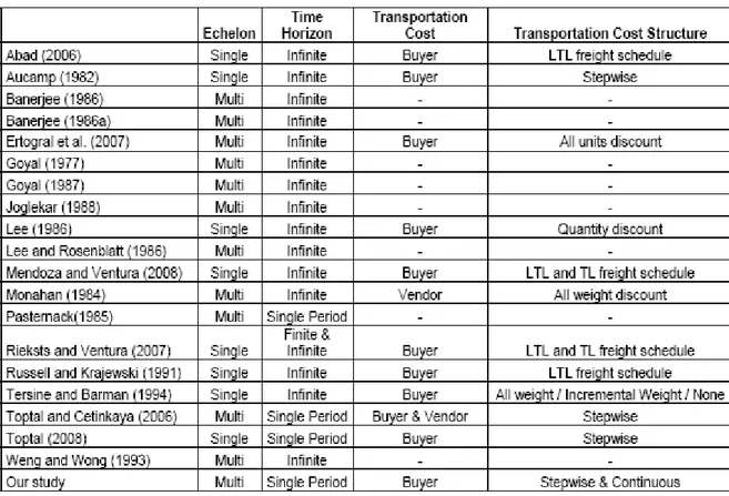
2.1 Paper classifications according to the number of echelons, problem’s time horizon, location and structure of the transportation cost ...10

2.2 Paper classifications according to the demand, wholesale price and unit cost structures.. 11

2.3 Paper classifications according to the type of the vendor and decision variables...11

6.1 Expected profits of the parties resulting from the retailer’s optimal replenishment decision for various values of R...58

6.2 Expected profits of the parties resulting from the retailer’s optimal replenishment decision for various values of R...59

6.3 Expected profits of the parties resulting from the retailer’s optimal replenishment decision for various values of s and R = 120 ...60

6.4 Expected profits of the parties resulting from the retailer’s optimal replenishment decision for various values of s and R = 180 ...61

(9)

Chapter 1 INTRODUCTION

Freight transportation is a significant component of the global economy. United States (US) and European Union (EU) hold the first two places in the world for their freight transportation expenditures. Freight shipping costs have been over 10% of the US Gross Domestic Product (GDP) in 2007 [23]. In EU countries, volume of the freight transportation per ton/km is expected to increase by 78% from 2000 to 2020, while the EU GDP is expected to grow by 60% in the same period [13]. In Turkey, as an EU candidate, freight transportation by road is expected to increase by 148% from 2004 to 2020 and its usage among all transportation paths (road, air, sea) is expected to increase from 81.2% in 2004 to 84.3% in 2020 [16].

In light of the above statistics, minimization of shipping costs presents an important opportunity for companies to improve their profits. This requires an effort for all parties involved in the supply chain ranging from retailers to distributors to transporter companies. Integration of inventory replenishment and transportation decisions, aggregation of different products across suppliers or buyers, efficient routing decisions are some important tools to decrease transportation costs. Minimization of freight costs for the parties who utilize this function is a highly explored topic in recent supply chain studies. However, there is limited research suggesting operating policies for companies that undertake this functionality. With

(10)

the increasing oil prices, uncertainty in the market and the raising competition among transporter companies, this topic has become well worth to study. The objectives of this thesis are to suggest methods for freight transporters to make their pricing decisions and to quantify the savings that can be achieved through these decisions.

With the above objectives in mind, we consider a system that consists of a retailer, a truckload (TL) carrier and a less than truckload (LTL) carrier. The retailer purchases the services of these carriers for inbound transportation and makes his/her replenishment decisions considering the related transportation costs and capacities. The TL carrier charges a fixed cost per truck regardless of whether the truck is fully or partially loaded. The LTL carrier charges in proportion to the number of units shipped. By loading as many quantities as possible in a truck, the retailer may get advantage of economies of scale inherent in fixed cost of each truck. However, this can happen to the extent that increased quantities do not raise the inventory related costs. If the quantity to be shipped does not justify the fixed cost of an additional truck, then the retailer uses the LTL carrier.

In the setting of the problem of interest, both the TL and the LTL carrier have their own costs. Besides the fixed costs associated with a transaction, the TL carrier incurs a cost for each truck utilized and the LTL carrier incurs a cost per unit shipped. The TL carrier and the LTL carrier announce their pricing schedules before the retailer decides on his/her replenishment decision.

In this thesis, we first model and solve the retailer’s replenishment problem under the given pricing decisions of the TL and the LTL carrier. Due to the complex structure exhibited by the retailer’s expected profit function, this analysis follows by investigating the structural properties of the profit function, which then leads to a characterization of the optimal solution. As it will be discussed in Chapter 3, the model and its solution can be used not only for the specific setting in this thesis but it also applies to a more general class of problems. In the later parts of the thesis, we study the pricing problems of the TL carrier and the LTL carrier

(11)

More specifically, we first study the problem of the TL carrier to determine the price he/she will charge for a single truck with the objective of maximizing his/her own profits given the LTL carrier’s pricing schedule. Secondly, for a similar objective for the LTL carrier, we study his/her problem to determine the price to be charged for the shipment of a single unit given the TL carrier’s pricing schedule. The analysis for the two transportation pricing problems follows based on two different characterizations of the retailer’s optimal response and structural properties of his/her objective function, which are discussed in Chapter 4.

In addition to an analytical investigation of the retailer’s replenishment problem and the carriers’ pricing problems, we illusrate over numerical examples the savings that can be achieved by the retailer as a result of jointly optimizing replenishment and transportation costs. We show that substantial savings can be achieved by the retailer in this setting due to the integrated model. We also illusrate the opportunity of savings for the TL carrier and the LTL carrier by carefully deciding on the value of their transportation services. We show that the TL carrier and the LTL carrier may increase their expected profits by percentages amounting to 27% and 20%, respectively. Another contribution of this thesis is that, we show the savings that can be achieved if the TL carrier and the LTL carrier coordinate. This can specifically be applicable to a situation where the truckload and the less-than-truck load transporation services are provided by the same company. Finally, we numerically show the impact of coordination between the retailer and one of the carriers.

The remainder of the thesis is organized as follows: In Section 2, a review of the related literature is provided. In Section 3, a detailed discussion of the problem definition and the mathematical models are presented. Section 4 is devoted to the analysis of the retailer’s replenishment problem. In Section 5, the pricing problems of the TL and the LTL carriers are analyzed. The results of a numerical study for the transportation pricing problems are reported in Section 6. Finally, the conclusions of this study are summarized in Section 7 in relation to the future research directions.

(12)

Chapter 2 LITERATURE REVIEW

Integration of transportation and inventory decisions has recently attracted significant attention from both the academia and the industry. It has been shown that significant savings can be achieved if the decisions associated with these supply chain functions are coordinated. The research in this thesis is closely related to the group of studies (Aucamp [2], Lee [11], Toptal [22]) which model transportation costs and constraints within the replenishment problem. The underlying replenishment problem in the thesis is different from the ones in the existing research in the fact that, the setting of interest herein considers the existence of two modes of transportation. The closest to our setting is the one that is analyzed by Rieksts and Ventura [18], however, in their modeling, demand is deterministic and the planning horizon is infinite. Another matter that is of importance in this thesis is transportation pricing. To our best knowledge, there is no study in the literature on transportation pricing.

Integrated inventory and transportation models will be reviewed in section 2.1. In addition to the concept of coordinating inventory and transportation decisions for a single echelon, this thesis puts forward the idea of coordinating these functions between different parties in the supply chain. Therefore, a closely related area of the literature is coordination, which will be reviewed in Section 2.2.

(13)

2.1 Transportation Issues

Aucamp [2] extends the standard EOQ model to the case where freight costs are determined by the integer number of carloads required to fill the order. Proposed solution method to determine the optimal solution yields three candidate solutions and the best of three is found by picking the one with the least cost. Aucamp [2] finds out that the optimal solution is not far away from the standard EOQ. In fact, the optimal solution involves a shipment that either uses the same number of cars as EOQ, or one less car.

Carter and Ferrin [6] focus on the importance of including transportation costs in the optimal inventory-lot sizing decisions. The authors advocate the buyer to manage the inbound transportation. They give some company examples from the practice to support their decisions. They conclude that substantial reductions in the freight rate can be obtained even with small increases in order quantity. Also, when shipment charges are constant for any order quantity that falls between a weight break quantity and the next discount minimum quantity suggests that order quantities (inventories) could be decreased without increasing transportation costs.

Rieksts and Ventura [18] analyze theoretical inventory models with constant demand rate and two transportation modes. The transportation options are truckloads (TL) with fixed costs, less than truckloads (LTL) with a constant per unit, or using a combination of both modes simultaneously. They derive optimal algorithms for single stage models over both an infinite and a finite planning horizon. They find out that optimal order interval should be in the same range with the optimal order interval of classical EOQ model and optimal order interval can either be one of the breakpoints or one of the minimizers of the average total cost functions with transportation costs. Mendoza and Ventura [14] extend the work done by Rieksts and Ventura to the case where all units or incremental quantity discount structures exist. They derive the optimal algorithms for each quantity discount structure for single stage models over an infinite planning horizon.

(14)

Lee [11] proposes algorithms on the classical EOQ model with setup cost including a fixed cost and freight cost. There is a quantity discount in freight costs. Assumptions of the proposed model are the same as the EOQ model except for the setup structure. Lee [11] refers his proposed model as the general model. The author also talks about some special cases of the general model. It is assumed that in special case called Special Model 1, basic charge paid for the first P units is greater than the incremental charge paid for each P more units. In special case called Special Model 2, basic charge is assumed to be equal to the incremental charge. In this study, the author proposes two algorithms to find the optimal order quantity. First algorithm can be used to solve the general model. Second algorithm, which is proposed for Model 2, is more efficient. It compares three possible candidates for the optimal solution and selects the one with the least cost depending on some conditions.

The use of the actual transportation cost function, complete with ranges of over-declared shipments, requires a modification to the standard procedures for determining the optimal purchase order quantity. Russell and Krajewski [19] present an analytical procedure for finding the order quantity that minimizes total purchase costs which reflect both transportation economies and quantity discounts. They find out that the optimal purchase order quantity will be one of the four following possibilities: (1) the valid economic order quantity (EOQ), (2) a purchase price breakpoint in excess of valid EOQ, (3) a transportation rate breakpoint in excess of valid EOQ, (4) a modified EOQ which provides an over-declared shipment in excess of valid EOQ. They also develop an algorithm which systematically explores these four possibilities. Abad [1] extend the work done by Russell and Krajewski [19] to the case where there is a temporary price reduction (TPR) offered by the supplier. Abad considers the buyer’s response to a TPR when the buyer is responsible for paying for freight. Abad models freight costs using the freight tariffs offered by public carriers in the practice. The author develops a search procedure for determining the optimal purchase lot size for the buyer in response to the TPR offered by the supplier.

(15)

weight freight, incremental quantity/incremental freight, all units quantity/incremental freight and incremental quantity/all-weight freight discount pairs are investigated. The authors also deal with single and no discount conditions in the paper.

2.2 Coordination Issues

Monahan [15] analyzes how a supplier can structure the terms of an optimal quantity discount schedule. Monahan [15] shows that supplier can increase his/her net profit by changing the ordering behavior of the buyer to increase his/her order size by a specific rate. It is shown that the optimal order increase rate is both dependent on the supplier’s order processing/manufacturing setup cost and the buyer’s fixed order processing cost. Lee and Rosenblatt [12] generalize Monahan’s model to relax the implicit assumption of a lot-for-lot policy adopted by the supplier and to incorporate constraints imposed on the amount of discount that can be offered. Lee and Rosenblatt [12] also find out that lot-for-lot policy is optimal when the setup costs and holding costs of both the supplier and buyer are equal. Goyal [9] criticizes Lee and Rosenblatt’s way to impose constraints on discount amount offered by the supplier. His assertion is that supplier may offer price discounts lower than the purchase price because high discounts on purchase prices may lead to greater economies of scale for the supplier [5, 9].

Banerjee [4] improves Monahan’s quantity discount model by considering supplier as a manufacturer. This means that supplier will hold finished goods inventory until the order is shipped to the buyer. Banerjee shows that Monahan’s model tends to overestimate the value of optimal order increase rate if the supplier is a manufacturer and claims that supplier will offer quantity discounts to the buyer to order smaller quantities which is not seen in practice a lot [4, 5]. Joglekar [10]criticizes Monahan’s one-item, one-customer and one-supplier model and judges Monahan’s implicit assumptions as unreasonable. Joglekar [10] shows that it is not economically beneficial for the supplier to match his/her production frequency with buyer’s ordering frequency if the supplier’s manufacturing setup costs are substantially larger than buyer’s ordering costs. If these are of similar magnitude, Monahan’s model does not have

(16)

much practical significance even though Monahan’s assumptions hold. Supplier can increase his/her profit more by considering a better production lot size policy instead of considering quantity discounts.

Weng and Wong [24] develop general models for the supplier’s all-unit quantity discount policy. The models developed deal with four major issues: (a) one buyer or multiple buyers, (b) constant or price elastic demand, (c) the relationship between supplier’s ordering or production policy and the buyer’s ordering size, (d) supplier is either a manufacturer or a wholesaler. Objectives of these models are either the supplier’s profit improvement or the supplier’s increased profit share analysis. They also develop algorithms to find the optimal decision policies. This paper provides the supplier with both the optimal all-unit quantity discount policy and the optimal production (or ordering) policy.

Goyal [8] models the replenishment problems of the single buyer/ single vendor systems using independent (decentralized) and integrated (centralized) approaches under the following assumptions: Buyer demand is deterministic and constant, no stockouts are permitted, vendor is not a manufacturer, buyer and vendor replenishment lead times are zero and minimization of the variable cost is the criterion of optimality. Goyal [8] finds out that total cost of centralized policy can not be greater or equal to the total cost of decentralized policy. Another important result in the paper is that, in centralized policy, buyer will order less frequently but in larger sizes. Using these results, the author concludes that vendor and buyer can make some agreements to get the advantage of the centralized solution. Banerjee [3] also focuses on the replenishment decisions in a vendor, buyer and single-product environment under the following assumptions; vendor is a manufacturer, there is a replenishment lead time, cycle times of the vendor and the buyer are same, order quantity of vendor is an integer multiple of the order quantity of the buyer . This paper develops a joint economic lot size model for a special case where vendor produces to order for a purchaser on a lot-for-lot basis under deterministic conditions. It is shown that a jointly optimal ordering policy, together with an appropriate price adjustment, can be beneficial for both parties or, at

(17)

Pasternack [17] considers the pricing decision faced by a producer of a commodity with a short shelf or demand life in a newsboy setting under the following assumptions; retailer will place only one order with the manufacturer, retailer will sell the product until his/her inventory is depleted, or the shelf life is exhausted. Manufacturer’s selection of the amount per unit charged to the retailer, the per unit credit for returned goods, and the percentage of purchased goods allowed to be returned are critical in achieving channel coordination and maximizing total profits. Pasternack [17] shows that the policy of a manufacturer allowing unlimited returns for full credit and the policy of a manufacturer allowing no returns are system suboptimal. On the other hand, a policy for unlimited returns at partial credit will be system optimal for appropriately chosen cost values. This policy can also achieve channel coordination in a multi-retailer environment.

Toptal and Çetinkaya [21] consider the coordination problem between a vendor and a buyer operating under generalized replenishment costs that include fixed costs as well as stepwise freight costs. They study the stochastic demand, single period setting where the buyer must decide on the order quantity to satisfy the random demand for a single item with a short product life cycle. They develop two models and derive the optimal order quantities both under decentralized and centralized settings. In the first model, they incorporate truck costs for the vendor only. In the second model, they incorporate truck costs both for the buyer and the vendor. Unlike the earlier research in this area, they prove that the vendor’s expected profit is not increasing in buyer’s order quantity. Their analysis show that the vendor can improve his/her profits by using an appropriate tariff schedule or a vendor managed delivery contract (VMD). Under VMD contract, vendor covers the buyer’s transportation expenses. They show that a VMD arrangement potentially improves the centralized solution. Toptal [22] extend the work done by Toptal and Çetinkaya [21] by analyzing a single echelon replenishment problem under a general replenishment cost structure that includes stepwise freight costs and all-units quantity discounts. The author proves several useful properties of the expected profit function and utilizes these properties to develop a computational solution approach to find the optimal order quantity. The solution procedures developed in this paper can easily be applied to multi-echelon settings.

(18)

Ertogral et al. [7] analyze the single vendor-single buyer problem under equal-size shipment policy. Two new models that integrate the transportation cost explicitly are developed. The transportation cost is considered to be in an all-unit-discount format for the first model. The option of over declaring a shipment to exploit the transportation cost structure is explored in the second model. Two important conclusions can be derived from this paper. First, savings can be realized by explicitly integrating transportation cost into the supply chain under consideration, depending on the transportation contribution to the total cost. Second, production and inventory decisions are affected when transportation is considered explicitly in the model. Tables 2.1, 2.2 and 2.3 classify the papers reviewed in this thesis.

Table 2.1 Paper classifications according to the number of echelons, problem’s time horizon,

(19)

Table 2.2 Paper classifications according to the demand, wholesale price and unit cost structures

(20)

Chapter 3 PROBLEM DEFINITION

In this study, we consider a system that includes a retailer and two carriers. The retailer operates in a Newsboy setting. That is, he/she makes a single replenishment decision at the beginning of a period during which he/she faces random demand. If the order quantity Q is greater than the demand, then excess items are salvaged at a $ v unit revenue. If it is less than the demand, then the retailer incurs a unit lost sale cost of $b. The retailer pays for the transportation of incoming materials. There are two modes of transportation, a TL carrier and a LTL carrier. The TL carrier charges $R per each truck whether it is fully or partially loaded. Each truck has a capacity of carrying P units and the TL carrier has ample number of trucks available. The LTL carrier charges $s per unit where R _s _R.

P< < That is, for carrying a truck

load of items, using the TL carrier is always less costly than using a LTL carrier. However, utilizing a truck has more costs when the quantity to be carried is less thanR s. More explicitly, the transportation cost of the retailer for replenishing Q units is given by

( )

min

{

(

)

,

(

1

)

}

C Q = s Q iP− +iR i+ R or

( )

Q min , Q , C Q R R s Q P P P ⎧ ⎛ ⎞⎫ ⎢ ⎥ ⎢ ⎥ =_{⎢ ⎥} + _⎨ _⎜ −_{⎢ ⎥} _⎟_⎬ ⎣ ⎦ ⎩ ⎝ ⎣ ⎦ ⎠⎭

(21)

where iP≤ < +Q

( )

i 1 P such that i∈

{ }

0 ∪ Z+. Here, Z is the set of all positive integers. +

The above expression can be rewritten either as

(

)

s Q iP− +iR if iP Q R iP s ≤ < + C Q

( )

=

( )

1

( )

i+1 R if R iP Q

(

i 1 ,

)

P s + ≤ < + or as Q Q s Q P R P P ⎛ ₋⎢ ⎥ ⎞₊⎢ ⎥ ⎜ _⎢_⎣ _⎥_⎦ ⎟ _⎢_⎣ _⎥_⎦ ⎝ ⎠ if Q _R Q P Q P P s P ⎢ ⎥ _{≤ <} ₊⎢ ⎥ ⎢ ⎥ ⎢ ⎥ ⎣ ⎦ ⎣ ⎦ C Q

( )

= Q R P ⎡ ⎤ ⎢ ⎥ ⎢ ⎥ if Rs+_⎣⎢⎢QP_⎦⎥⎥P≤ <Q ⎡_⎢⎢QP_⎥⎤⎥P,

For given values of R, P and s, retailer’s expected profit for replenishing Q units, i.e.

( )

, H Q is given by G Q

( )

−C Q

( )

where

( ) (

) (

)

(

) (

)

( ) . Q G Q r v c v Q r b v Q x f x dx ∞ = − μ − − + + −

∫

−

( )

2

The TL carrier and the LTL carrier incur fixed setup costs as long as the retailer utilizes their services. Once the retailer decides on his/her replenishment quantity and how much of it will be carried by which carrier, the carriers are in charge of performing the required service. Namely, for long term business and customer satisfaction, neither the TL carrier nor the LTL carrier rejects an order even if the revenue does not cover the fixed costs implying that it is not a profitable transaction.

(22)

Before introducing TL carrier’s and LTL carrier’s expected profit functions, we next summarize the notation introduced so far and that will be used in the remaining parts of the text.

:r Retail price per unit.

:b Retailer’s per unit lost sale cost.

:v Salvage value of an item unsold at the retailer. :c Wholesale price per unit.

R Per truck shipping price that the TL carrier charges. : R The TL carrier’s fixed cost for utilizing one truck. : P Capacity of a truck in number of units. :

:s Per unit shipping price that the LTL carrier charges. :s The LTL carrier’s cost for shipping one unit.

:

TL

K Setup cost of the TL carrier. K_LTL: Setup cost of the LTL carrier.

Q: Retailer’s replenishment quantity.

C Q

( )

: Transportation cost of the retailer for replenishing Q units. G Q Retailer’s expected profit function excluding the truck costs.

( )

: H Q

( )

: Retailer’s expected profit function.

Q Quantity transported using the TL carrier. ₁:

Q₂: Quantity transported using the LTL carrier.

∏_TL

(

Q R,

)

: TL carrier’s profit if the retailer replenishes Q units.

(

, :

)

LTL Q s

∏ LTL carrier’s profit if the retailer replenishes Q units. X : Random variable showing demand in a single period. f x

( )

: Probability density function of demand.

(23)

The TL carrier’s profits ∏_TL

( )

Q in this system are given by i×

(

R−R

)

−K_TL if iP Q R iP s ≤ < + and Q>0

(

,

)

TL Q R ∏ =

( )

i+ ×1

(

R−R

)

−K_TL if R iP Q

(

i 1 ,

)

P s + ≤ < +

( )

3

0

otherwise,

which can alternatively be written as

Q

(

R R

)

K_TL P ⎢ _{⎥ × − −} ⎢ ⎥ ⎣ ⎦ if ⎢⎢_⎣QP⎥_⎦⎥P≤ <Q Rs +_⎣⎢⎢QP_⎦⎥⎥P and Q>0

(

,

)

TL Q R ∏ = Q

(

R R

)

K_TL P ⎡ _{⎤ × − −} ⎢ ⎥ ⎢ ⎥ if Rs+⎢_⎣⎢QP_⎦⎥⎥P≤ <Q ⎡⎢_⎢QP⎤⎥_⎥P,

0

otherwise.

Similarly, the LTL carrier’s profits ∏_LTL

( )

Q are

(

s− ×s

) (

Q iP−

)

−K_LTL if iP Q R iP s < < + ∏_LTL

(

Q s,

)

=

( )

4

0

otherwise,

which can alternatively be represented as

(

s s

)

Q Q P K_LTL P ⎛ ⎢ ⎥ ⎞ − ×_⎜ −_⎢ _⎥ _⎟− ⎣ ⎦ ⎝ ⎠ if Q _R Q P Q P P s P ⎢ ⎥ _{< <} ₊⎢ ⎥ ⎢ ⎥ ⎢ ⎥ ⎣ ⎦ ⎣ ⎦ ∏_LTL

(

Q s,

)

=

0

otherwise.

(24)

Expression

( )

1 implies that, if iP Q R iP,

s

≤ < + then Q₁=iP and Q₂ = −Q iP. Similarly, if

(

1 ,

)

R _iP _Q _i _P

s + ≤ < + then Q1= +( 1)i P and Q2 = Note also that, TL carrier does not get 0.

any profit from this transaction if

(

)

1 KTL R R P Q ≤ − ⎡ ⎤ ⎢ ⎥

⎢ ⎥ and the LTL carrier does not get any profit

from this transaction if ₂

₍

KLTL

₎

. s s

Q

−

≤

In order to write a more explicit expression for the retailer’s expected profit function, we introduce the following two functions over Q≥0 and j∈

{ }

0 ∪ Z+ :

(

)

( ) (

)

1 , H Q j =G Q −s Q− jP − jR

( )

5 and

(

)

( )

2 , . H Q j =G Q − jR

( )

6

It turns out that we have

( )

1 , H Q i if iP Q R iP s ≤ < + H Q

( )

=

( )

7

(

)

2 , 1 H Q i+ if R iP Q

(

i 1 .

)

P s + ≤ < +

Given the values of R and s, the retailer solves the following problem to decide on his/her replenishment quantity. max Q

( )

H Q s.t. Q≥0.

(25)

Let the optimal solution of the above problem be Q*

( )

R s, . In this thesis, we first

analyze the structural properties of H Q and propose a finite time exact solution procedure

( )

for finding Q*

( )

R s, given the values of R and s. Then we study the underlying

transportation pricing problems that the TL and LTL carriers face. Namely, given the TL carrier’s per truck shipping price R, we study the problem of the LTL carrier in deciding the value of s. We refer to this problem as LTLP. Then given the LTL carrier’s per unit transportation charge, we study the problem of TL carrier in deciding the value of R, referred to as Problem TLP. Throughout this analysis, we assume that the two carriers know the retailer’s inventory related costs and hence they predict the response of the retailer in terms of his/her order quantity, i.e., the value of Q*

( )

R s, .

The pricing problems of the TL carrier as described above can be formulized as follows: TLP: max R

(

)

* , , TL Q R s R ∏ s.t. R<sP, R>s.

Similarly, the pricing problem of the LTL carrier is given by

LTLP: max s

(

)

(

* , ,

)

LTL Q R s s ∏ s.t. R _s _R. P< <

In the next section, we study the retailer’s replenishment problem to characterize his/her response to given values of R and s.

(26)

Chapter 4 RETAILER’S INTEGRATED INVENTORY

REPLENISHMENT AND

TRANSPORTATION PROBLEM

In this section, we propose an algorithm to find the maximizer of H Q

( )

. As seen in Figure 4.1, H Q

( )

is a piecewise function. Therefore, our analysis will follow by proving some of

its structural properties. Regarding Expression

( )

2 , we would like to note that the analysis in this chapter will use the fact that G(Q) is a strictly concave function of Q

2 2 i.e., d G Q( ) 0 dQ ⎛ ⎞ ⎜ ⎟

⎝ < ⎠. Therefore, the analysis herein is not restricted to the Newsboy setting but

it also applies to a more general class of problems where the production/inventory related expected profits of the retailer is strictly concave. The following lemma indicates the continuity of H Q

( )

which forms the fundamental component of our analysis for finding the

optimal solution of the replenishment problem.

(27)

Proof: Since H Q j and ₁

(

,

)

H₂

(

Q j are continuous functions of Q for fixed j, we will prove ,

)

that H Q

( )

is continuous at the breakpoints which are iP and R iP,

s + i

{ }

0 .

+

∈ ∪ Z Let us first consider Q R iP,

s

= + i∈

{ }

0 ∪ Z+. Note that, we have

lim R Q iP s ⎛ ⎞ →_⎜ + _⎟ ⎝ ⎠ −

( )

1 , . R H Q H iP i s ⎛ ⎞ = _⎜ + _⎟ ⎝ ⎠

Using Expression

( )

5 , it follows that

lim R Q iP s ⎛ ⎞ →_⎜ + _⎟ ⎝ ⎠ −

( )

(

)

, R R H Q G iP s iP sP R i s s ⎛ ⎞ ⎛ ⎞ = _⎜ + _⎟− _⎜ + _⎟+ − ⎝ ⎠ ⎝ ⎠ which leads to lim R Q iP s ⎛ ⎞ →_⎜ + _⎟ ⎝ ⎠ −

( )

(

1 .

)

R H Q G iP R i s ⎛ ⎞ = _⎜ + _⎟− + ⎝ ⎠

Expression

( )

6 implies that the right hand side of above equality is H₂

(

R iP i, 1

)

s + + which

is equal to _H

(

R _iP

)

.

s +

Next, we will show that H Q

( )

is continuous at Q=iP, i∈Z As Q approaches to iP from +.

the below, the one sided limit of H Q

( )

is given by,

( )

lim Q→ iP −

( )

2

(

, .

)

(28)

Using Expression

( )

6 , we have

( )

lim Q→ iP −

( )

. H Q =G iP −iR

Rewriting the right-hand side of the above equality as G iP

( )

−siP i sP+ ( −R), it can be observed from Expression

( )

5 that

( )

lim Q→ iP −

( )

1

(

,

)

( )

. H Q =H iP i =H iP

■

2480 2530 2580 2630 2680 2730 650 662 674 686 698 710 722 734 746 758 770 782 794 806 818 830 842 854

Figure 4.1 An illustration of the retailer’s expected profit function

Since G Q

( )

is a strictly concave function, it follows from Expressions

( )

5 and

( )

6 that

(

)

1 ,

H Q j and H₂

(

Q j are strictly concave functions over Q for fixed j. Therefore, they ,

)

have unique maximizers. Let q* be the maximizer of G Q

( )

. It can be observed that q* is also the unique maximizer of H₂

(

Q j, ,

)

∀.j Similarly, let z* be the unique maximizer of

H(Q)

(29)

(

)

1 , ,

H Q j ∀.j It follows from Expression

( )

5 that G z′

( )

* = The following lemma s.

characterizes the ordinal relationship between q* and z*.

Lemma 2 We have z*<q*.

Proof: Since q* is the unique maximizer of G Q

( )

, which is a strictly concave function of Q, we have G Q′

( )

> 0 ∀Q s.t. Q<q* and G Q′

( )

< 0 ∀Q s.t. Q>q*. By definition of z*, we

have G z′

( )

* = Since s. s>0, it follows that z*<q*.

■

In the following analysis, we will prove some structural properties of H Q

( )

to arrive

at an algorithm that finds Q*

( )

R s, . In this analysis, we say z* is realizable if there exists

{ }

0

i∈ ∪ Z+ such that iP Q R iP. s

≤ < + Similarly, q* is realizable if there exists i∈

{ }

0 ∪ Z+

such that R iP Q

(

i 1 .

)

P

s + ≤ < + In the next lemma, we show that z* dominates all order

quantities that are smaller than itself, therefore, in maximizing H Q

( )

, order quantities less

than z* should not be considered.

Lemma 3 We have H Q

( )

<H z

( )

* , ∀ <Q z*.

Proof: The proof will follow by considering the following two cases:

i) H z

( )

* =H₁

(

z i*,

)

where iP z* R iP s

≤ < + for some i∈

{ }

0 ∪ Z+. That is, z* is realizable.

ii) H z

( )

* =H₂

(

z i*, + where 1

)

R iP z*

(

i 1

)

P

s + ≤ < + for some i

{ }

0 .

+

∈ ∪ Z That is, z* is not realizable.

(30)

Case 1, z* is realizable: First, we will show that H z

( )

* >H Q

( )

, ∀Q s.t. jP z* R jP s

≤ < +

and .j≤ To complete the proof for Case 1, secondly, we will show that i H z

( )

* >H Q

( )

,

Q

∀ s.t. R jP z*

(

j 1

)

P

s + ≤ < + and j< i.

Let us start with Q such that jP Q R jP s

≤ < + and j≤ Since z* is the unique i. maximizer of H Q j₁

(

,

)

over Q, ∀j, we have

(

)

(

)

1 *, 1 , , H z j >H Q j jP Q R jP, s ≤ < + j≤ i.

( )

8

Using Expression

( )

5 , we further have

(

)

(

)

1 *, 1 *, , .

H z i >H z j ∀ < j i

( )

9

It follows from Expressions

( )

8 and

( )

9 that

(

)

(

)

1 *, 1 , ,

H z i >H Q j jP Q R jP, s

≤ < + j≤ i.

Recall from Expression

( )

7 that we have H Q

( )

=H Q j₁

(

,

)

for Q such that jP Q R jP. s

≤ < +

Therefore, the above expression implies

( )

* ,

H Q <H z ∀Q s.t. jP Q R jP s

≤ < + and j≤ i.

( )

10

Now, let us consider Q such that R jP Q

(

j 1

)

P

s + ≤ < + and j< Recall that i.

(

)

2 ,

H Q j is a strictly concave function of Q for fixed ,j and q* is its unique maximizer.

(31)

(

)

(

)

2 , 2 , ,

H Q j <H jP j ∀ <Q jP and j≤ i.

( )

11

Note also that we have H₁

(

jP j,

)

=H₂

(

jP j, .

)

Combining this with the fact that

* z ≥iP≥ jP further leads to

(

)

(

)

(

)

1 *, 1 , 2 , , H z j ≥H jP j =H jP j ∀ ≤j i.

( )

12

Using Expressions

( )

11 and

( )

12 , we conclude that

(

)

(

)

1 *, 2 , ,

H z j >H Q j ∀ <Q jP and j≤ i.

The above expression implies that

(

)

(

)

1 *, 2 , ,

H z j >H Q j ∀Q s.t. R

(

j 1

)

P Q jP

s + − ≤ < and 1≤ ≤j i,

which can be rewritten as

(

)

(

)

1 *, 2 , ,

H z j >H Q j ∀Q s.t. R jP Q

(

j 1

)

P

s + ≤ < + and 0≤ <j i.

( )

7 that, we have H Q

( )

=H₂

(

Q j,

)

for Q such that

(

1 .

)

R _jP _Q _j _P s + ≤ < + Therefore,

( )

*

( )

, H z >H Q ∀Q s.t. R jP Q

(

j 1

)

P s + ≤ < + and 0≤ <j i.

Combining Expression

( )

10 with the above result, we conclude that H z

( )

* >H Q

( )

,

*

Q z

∀ < if ∃ ∈i

{ }

0 ∪ Z such that + iP Q R iP. s

(32)

Case 2, z* is not realizable: The proof of this case is similar to that of Case 1. We will first show that H z

( )

* >H Q

( )

, ∀Q s.t. jP Q R jP

s

≤ < + and j≤ To complete the proof for i. Case 2, secondly, we will show that H z

( )

* >H Q

( )

, ∀Q s.t. R jP Q

(

j 1

)

P

s + ≤ < + and

*.

Q<z

Let us start with Q such that _jP _Q R _jP s

≤ < + and j≤ The fact that i.

( )

* 2

(

*, 1

)

H z =H z i+ implies

(

)

(

)

2 *, 1 1 *, .

H z i+ ≥H z i

Since H₁

(

z i*,

)

>H₁

(

z*, ,j

)

∀ <j i, and z* is the unique maximizer of H Q j1

(

,

)

over Q, we

have

(

)

(

)

1 *, 1 , , H z i >H Q j ∀Q s.t. jP Q R jP s ≤ < + and j≤ i. Therefore,

(

)

(

)

2 *, 1 1 , , H z i+ >H Q j ∀Q s.t. jP Q R jP s ≤ < + and j≤ i,

( )

13 and hence,

( )

*

( )

, H z >H Q ∀Q s.t. jP Q R jP s ≤ < + and j≤ i.

( )

14

Now, let us consider Q such that R jP Q

(

j 1

)

P

s + ≤ < + and Q<z*. Since q* is the

unique maximizer of H₂

(

Q j,

)

over Q and z*<q*, it follows that

(33)

( )

*

( )

, H z >H Q ∀Q s.t. R iP Q z*. s + ≤ <

( )

15 We have q*>z*>iP, therefore,

(

)

(

)

2 , 2 , , H Q j <H jP j ∀ <Q jP, 1≤ ≤j i.

( )

16

Expression

( )

13 implies that

(

)

(

)

2 *, 1 1 , ,

H z i+ >H jP j ∀ ≤j i.

( )

17

Using the fact that H₁

(

jP j,

)

=H₂

(

jP j, ,

)

Expressions

( )

16 and

( )

17 lead to

(

)

(

)

2 *, 1 2 , , H z i+ >H Q j ∀Q such that R jP Q

(

j 1

)

P s + ≤ < + and j< i, and hence,

( )

*

( )

, H z >H Q ∀Q such that R jP Q

(

j 1

)

P s + ≤ < + and j< i.

( )

18

Combining Expressions

( )

15 and

( )

18 , we have

( )

*

( )

,

H z >H Q ∀Q such that R jP Q

(

j 1

)

P

s + ≤ < + and Q<z*.

( )

19

■

In the next lemma, we show that q* dominates all order quantities that are greater than itself, therefore, in maximizing H Q

( )

, order quantities greater than q* should not be considered.

(34)

Lemma 4 We have H Q

( )

<H q

( )

* , ∀ >Q q*.

Proof: The proof will follow by considering the following two cases:

i) H q

( )

* =H₂

(

q i*, + where 1

)

R iP q*

(

i 1

)

P s + ≤ < + for some i

{ }

0 . + ∈ ∪ Z That is, q* is realizable. ii) H q

( )

* =H q i₁

(

*,

)

where iP q* R iP s

≤ < + for some i∈

{ }

0 ∪ Z+. That is, q* is not

realizable.

Case 1, q* is realizable: First, we will show that H q

( )

* >H Q

( )

, ∀Q s.t.

(

1 ,

)

R _jP _Q _j _P

s + ≤ < + j i≥ and Q>q*. Secondly, we will show that H q

( )

* >H Q

( )

, Q

∀ s.t. jP Q R jP,

s

≤ < + j> and this will complete the proof for Case 1. i,

Let us start with Q such that R jP Q

(

j 1 ,

)

P

s + ≤ < + j i≥ and Q>q*. Since q* is the

unique maximizer of H₂

(

Q j,

)

over Q, ∀j, we have

(

)

(

)

2 *, 1 2 , 1 ,

H q j+ >H Q j+ R jP Q

(

j 1 ,

)

P

s + ≤ < + j i≥ and Q>q*.

( )

20

Using Expression

( )

6 , we further have

(

)

(

)

2 *, 1 2 *, 1 , .

H q i+ >H q j+ ∀ > j i

( )

21

It follows from Expressions

( )

20 and

( )

21 that

(

)

(

)

2 *, 1 2 , 1 ,

H q i+ >H Q j+ R jP Q

(

j 1 ,

)

P

(35)

( )

7 that we have H Q

( )

=H₂

(

Q j, + for Q such that 1

)

(

1 .

)

R _jP _Q _j _P

s + ≤ < + Therefore, the above expression implies

( )

* ,

H Q <H q ∀Q s.t. R jP Q

(

j 1 ,

)

P

s + ≤ < + j i≥ and Q>q*.

( )

22

Now, let us consider Q such that jP Q R jP s

≤ < + and j> Recall that i. H Q j₁

(

,

)

is a

strictly concave function of Q for fixed ,j and z* is its unique maximizer. Since

(

i+1

)

P>q*>z*, it follows that

(

)

(

)

1 , 1 , ,

H Q j <H jP j ∀ >Q jP and j> i.

( )

23

Note also that we have H₁

(

jP j,

)

=H₂

(

jP j, .

)

Combining this with the fact that

(

1

)

* jP≥ +i P>q further leads to

(

)

(

)

(

)

2 *, 2 , 1 , , H q j >H jP j =H jP j ∀ >j i.

( )

24 Using Expressions

( )

23 and

( )

24 , we conclude that

(

)

(

)

2 *, 1 , ,

H q j >H Q j ∀ ≥Q jP and j> i.

The above expression implies that

(

)

(

)

2 *, 1 , ,

H q j >H Q j ∀Q s.t. jP Q R jP s

≤ < + and j>i.

( )

7 that, we have H Q

( )

=H Q j₁

(

,

)

for Q such that

.

R

jP Q jP

s

(36)

( )

*

( )

,

H q >H Q ∀Q s.t. jP Q R jP s

≤ < + and j>i.

Combining Expression

( )

22 with the above result, we conclude that H q

( )

* >H Q

( )

,

*

Q q

∀ > if ∃ ∈i

{ }

0 ∪ Z such that + R iP q*

(

i 1 .

)

P

s + ≤ < +

Case 2, q* is not realizable: The proof of this case is similar to that of Case 1. We will first show that H q

( )

* >H Q

( )

, ∀Q s.t. R jP Q

(

j 1

)

P

s + ≤ < + and j≥ To complete the proof i.

for Case 2, secondly, we will show that H q

( )

* >H Q

( )

, ∀Q s.t. jP Q R jP, s

≤ < + j i≥ and Q>q*.

Let us start with Q such that R jP Q

(

j 1

)

P

s + ≤ < + and j≥ The fact that i.

( )

* 1

(

*,

)

H q =H q i implies

(

)

(

)

1 *, 2 *, 1 .

H q i >H q i+

Since H2

(

q i*, + >1

)

H2

(

q*, j+1 ,

)

∀ >j i, and q* is the unique maximizer of H2

(

Q j,

)

over

Q, we have

(

)

(

)

2 *, 1 2 , 1 , H q i+ >H Q j+ ∀Q s.t. R jP Q

(

j 1

)

P s + ≤ < + and j≥ i. Therefore,

(

)

(

)

1 *, 2 , 1 , H q i >H Q j+ ∀Q s.t. R jP Q

(

j 1

)

P s + ≤ < + and j≥ i,

( )

25 and hence,

(37)

( )

*

( )

,

H q >H Q ∀Q s.t. R jP Q

(

j 1

)

P

s + ≤ < + and j≥ i.

( )

26

Now, let us consider Q such that jP Q R jP s

≤ < + and Q>q*. Since z* is the unique

maximizer of H Q j₁

(

,

)

over Q and z*<q*, it follows that H q i₁

(

*,

)

>H Q i₁

( )

, , ∀ >Q q*,

and hence,

( )

*

( )

, H q >H Q ∀Q s.t. q* Q R iP. s < < +

( )

27 We have

(

i+1

)

P>q*>z*, therefore,

(

)

(

)

1 , 1 , , H Q j <H jP j ∀ >Q jP, j>i.

( )

28 Expression

( )

25 implies that

(

)

(

)

1 *, 2 , ,

H q i >H jP j ∀ >j i.

( )

29

Using the fact that H1

(

jP j,

)

=H2

(

jP j, ,

)

Expressions

( )

28 and

( )

29 lead to

(

)

(

)

1 *, 1 , , H q i >H Q j ∀Q such that jP Q R jP s ≤ < + and j> i, and hence,

( )

*

( )

, H q >H Q ∀Q such that jP Q R jP s ≤ < + and j> i.

( )

30 Combining Expressions

( )

27 and

( )

30 , we have

( )

*

( )

,

H q >H Q ∀Q such that jP Q R jP s

(38)

■

Lemma 3 and Lemma 4 jointly imply that we should only focus on Q such that *z ≤ ≤Q q* while optimizing H Q

( )

. In Lemma 5 and Lemma 6, by a similar analysis, we further

eliminate some quantity values between z* and q*.

Lemma 5 Let Q be an order quantity such that z*< <Q q* and jP Q R jP, s

≤ < +

{ }

0 .

j∈ ∪ Z+ Then, we have H max z*, Q P H Q

( )

. P ⎛ ⎧ ⎢ ⎥ ⎫⎞_> ⎨ ⎬ ⎜ _{⎢ ⎥}_{⎣ ⎦} ⎟ ⎩ ⎭ ⎝ ⎠

Proof: Note that, if max z*, Q P z*, P ⎧ ⎢ ⎥ ⎫₌ ⎨ _{⎢ ⎥} ⎬ ⎣ ⎦ ⎩ ⎭ then s jP. R Q * z jP< < < + In this case, we

have H z

( )

* =H₁

(

z*, j

)

and H Q

( )

=H Q j₁

(

, .

)

Since z* is the maximizer of H Q j₁

(

,

)

over

Q, it follows that H₁

(

z*, j

)

>H Q j₁

(

,

)

, and hence, H z

( )

* >H Q

( )

.

If max z*, Q P Q P, P P ⎧ ⎢ ⎥ ⎫₌⎢ ⎥ ⎨ _{⎢ ⎥} ⎬ _{⎢ ⎥} ⎣ ⎦ ⎣ ⎦ ⎩ ⎭ then * . Q z P P ⎢ ⎥

< ⎢ ⎥_{⎣ ⎦} Expression

( )

7 implies that

( )

1

(

,

)

H Q =H Q j and H Q P H₁ Q P j, .

P P

⎛⎢ ⎥ ⎞₌ ⎛⎢ ⎥ ⎞ ⎜⎢ ⎥_{⎣ ⎦} ⎟ ⎜⎢ ⎥_{⎣ ⎦} ⎟

⎝ ⎠ ⎝ ⎠ It follows from the strict concavity of

(

)

1 ,

H Q j over Q and the fact that Q P z*, P ⎢ ⎥ > ⎢ ⎥ ⎣ ⎦ we have 1 , 1

(

,

)

, Q H P j H Q j P ⎛⎢ ⎥ ⎞_> ⎜_{⎢ ⎥}_{⎣ ⎦} ⎟ ⎝ ⎠ which implies H Q P H Q

( )

. P ⎛⎢ ⎥ ⎞_> ⎜⎢ ⎥_{⎣ ⎦} ⎟ ⎝ ⎠

■

(39)

Lemma 6 Let Q be an order quantity such that *z < <Q q* and R jP Q

(

j 1 ,

)

P

s + ≤ < +

{ }

0 .

j∈ ∪ Z+ Then, we have H min q*, Q P H Q

( )

. P ⎛ ⎧ ⎡ ⎤ ⎫⎞_> ⎨ ⎬ ⎜ _{⎢ ⎥}_{⎢ ⎥} ⎟ ⎩ ⎭ ⎝ ⎠ Proof: If min q*, Q P q*, P ⎧ ⎡ ⎤ ⎫₌ ⎨ _{⎢ ⎥} ⎬ ⎢ ⎥ ⎩ ⎭ then s jP Q q j P R ) 1 ( + < < ≤

+ ∗ _{. In this case, we have}

( )

* 2

(

*, 1

)

H q =H q j+ and H Q

( )

=H₂

(

Q j, +1 .

)

Since q* is the maximizer of H₂

(

Q j, +1

)

over Q, it follows that H₂

(

q*, j+ >1

)

H₂

(

Q j, +1 ,

)

and hence, H q

( )

* >H Q

( )

.

If min q*, Q P Q P, P P ⎧ ⎡ ⎤ ⎫₌⎡ ⎤ ⎨ _{⎢ ⎥} ⎬ _{⎢ ⎥} ⎢ ⎥ ⎢ ⎥ ⎩ ⎭ then * . Q q P P ⎡ ⎤

> ⎢ ⎥_{⎢ ⎥} It follows from the strict concavity of

(

)

2 ,

H Q j over Q and the fact that Q P q*, P ⎡ ⎤ < ⎢ ⎥ ⎢ ⎥ we have 2 , 1 2

(

, 1 ,

)

Q H P j H Q j P ⎛⎡ ⎤ _{+ >}⎞ ₊ ⎜⎢ ⎥_{⎢ ⎥} ⎟ ⎝ ⎠ which implies H Q P H Q

( )

. P ⎛⎡ ⎤ ⎞_> ⎜⎢ ⎥_{⎢ ⎥} ⎟ ⎝ ⎠

■

Lemma 5 and Lemma 6 imply that among the order quantities between z* and q*, we should only consider full truck loads. The following theorem provides a characterization of the retailer’s optimal order quantity.

Theorem 1 The order quantity which maximizes H Q

( )

is given by

( )

* , Q R s =arg max

( ) ( ) ( )

* , * , . . z* ,..., q* , z* ,..., q* . P P P P H z H q H kP s t k k ⎧ ₌_{⎡ ⎤} ⎢ ⎥ _∈⎧_{⎡ ⎤} ⎢ ⎥⎫⎫ ⎨ _{⎢ ⎥} _⎢_⎣ _⎥_⎦ ⎨_{⎢ ⎥} _⎢_⎣ _⎥_⎦⎬⎬ ⎩ ⎭ ⎩ ⎭

Proof: The proof follows from Lemmas

( ) ( ) ( )

3 , 4 , 5 and

( )

6 .

The above theorem implies that the retailer does not use the LTL carrier if both z* and

(40)

retailer only if the retailer orders z* and z* is realizable, or if the retailer orders q* and q* is not realizable. Because in all other cases, the retailer uses only the TL carrier. The following lemma further shows that in the second case (i.e., Q*

( )

R s, =q* and q* is not realizable), the

quantity shipped using the LTL carrier is zero.

Lemma 7 If there exists j, j∈

{ }

0 ∪ Z+ such that jP, s R * q

jP≤ < + that is q* is not realizable, then the retailer orders q* only if q* is an integer number of full truck loads.

Proof: Assume by the way of contradiction that the retailer orders q* and q* is not a full

truckload. Since jP q* R jP,

s

< < + we have H q

( )

* =H q₁

(

*, .j

)

It follows from the strict

concavity of H Q j₁

(

,

)

and the fact that z*<q*, there exists Q such that

* R jP Q q jP s < < < + and ₁ , q* ₁ *, q* . P P H ⎛_⎜Q _⎢⎢ ⎥_⎥⎞_⎟>H ⎛_⎜q _⎢⎢ ⎥_⎥_⎟⎞ ⎣ ⎦ ⎣ ⎦

⎝ ⎠ ⎝ ⎠ Note also that, we have

( )

1 * , q . P H Q =H ⎛_⎜Q ⎢_⎢ ⎥_⎥⎞_⎟ ⎣ ⎦

⎝ ⎠ Therefore, H Q

( )

>H q

( )

* , and hence, q* cannot be retailer’s

optimal order quantity.

■

Lemma 8 If ∃ j∈

{ }

0 ∪ Z+ such that R jP z*

(

j 1 ,

)

P

s + ≤ < + that is if z* is not realizable,

then it is not optimal.

Proof: If z* is not realizable, then we have R jP z*

(

j 1

)

P

s + ≤ < + for some j

{ }

0 .

+

∈ ∪ Z

This implies that H z

( )

* =H₂

(

z*, j+1 .

)

Since z*<q* and q* is the maximizer of

(

)

2 , 1 ,

H Q j+ it follows that there exists Q such that z*< <Q

(

j+1

)

P and

(

)

(

)

2 , 1 2 *, 1 .

Replenishment and transportation pricing decisions under two independent carriers with different modes