NETWORK-AWARE VIRTUAL MACHINE
PLACEMENT IN CLOUD DATA CENTERS
WITH MULTIPLE TRAFFIC-INTENSIVE
COMPONENTS
a thesis
submitted to the department of computer engineering
and the graduate school of engineering and science
of bilkent university
in partial fulfillment of the requirements
for the degree of
master of science
By
Amir Rahimzadeh Ilkhechi
July, 2014
I certify that I have read this thesis and that in my opinion it is fully adequate, in scope and in quality, as a thesis for the degree of Master of Science.
Assoc. Prof. Dr. ˙Ibrahim K¨orpeo˘glu (Advisor)
I certify that I have read this thesis and that in my opinion it is fully adequate, in scope and in quality, as a thesis for the degree of Master of Science.
Prof. Dr. ¨Ozg¨ur Ulusoy (Co–advisor)
I certify that I have read this thesis and that in my opinion it is fully adequate, in scope and in quality, as a thesis for the degree of Master of Science.
Prof. Dr. Uˇgur G¨ud¨ukbay
I certify that I have read this thesis and that in my opinion it is fully adequate, in scope and in quality, as a thesis for the degree of Master of Science.
Prof. Dr. Ahmet Co¸sar
Approved for the Graduate School of Engineering and Science:
Prof. Dr. Levent Onural Director of the Graduate School
ABSTRACT
NETWORK-AWARE VIRTUAL MACHINE
PLACEMENT IN CLOUD DATA CENTERS WITH
MULTIPLE TRAFFIC-INTENSIVE COMPONENTS
Amir Rahimzadeh Ilkhechi M.S. in Computer Engineering
Supervisors: Assoc. Prof. Dr. ˙Ibrahim K¨orpeo˘glu and Prof. Dr. ¨Ozg¨ur Ulusoy July, 2014
Following a shift from computing as a purchasable product to computing as a deliverable service to the consumers over the Internet, Cloud Computing emerged as a novel paradigm with an unprecedented success in turning
utility computing into a reality. Like any emerging technology, with its
advent, Cloud Computing also brought new challenges to be addressed. This work studies network and traffic aware virtual machine (VM) placement in Cloud Computing infrastructures from a provider perspective, where certain infrastructure components have a predisposition to be the sinks or sources of a large number of intensive-traffic flows initiated or targeted by VMs. In the scenarios of interest, the performance of VMs are strictly dependent on the infrastructure’s ability to meet their intensive traffic demands. We first introduce and attempt to maximize the total value of a metric named “satisfaction” that reflects the performance of a VM when placed on a particular physical machine (PM). The problem is NP-hard and there is no polynomial time algorithm that yields an optimal solution. Therefore we introduce several off-line heuristics-based algorithms that yield nearly optimal solutions given the communication pattern and flow demand profiles of VMs. We evaluate and compare the performance of our proposed algorithms via extensive simulation experiments.
Keywords: Cloud Computing, Virtual Machine Placement, Sink Node,
¨
OZET
YO ˇ
GUN TRAF˙I ˇ
GE SAH˙IP C
¸ OK SAYIDA B˙ILES
¸ENDEN
OLUS
¸AN BULUT VER˙I MERKEZLER˙I ˙IC
¸ IN MEVCUT
A ˇ
G KOS
¸ULLARINI G ¨
OZ ¨
ON ¨
UNE ALAN SANAL
MAK˙INE YERLES
¸T˙IRME
Amir Rahimzadeh Ilkhechi Bilgisayar M¨uhendisli˘gi, Y¨uksek Lisans
Tez Y¨oneticileri: Do¸c. Dr. ˙Ibrahim K¨orpeo˘glu ve Prof. Dr. ¨Ozg¨ur Ulusoy Temmuz, 2014
Hesaplamanın satın alınabilir bir ¨ur¨unden ˙Internet ¨uzerinde kullanıcılara sunulabilir bir hizmete d¨on¨u¸smesinin ardından, Bulut Bili¸sim yeni bir model olarak hizmetli hesaplamayı ger¸cekle¸stirmede e¸ssiz bir ba¸sarısıyla ortaya ¸cıkmı¸stır. Geli¸smekte olan herhangi bir teknoloji gibi, Bulut Bili¸sim de geli¸simiyle beraber ¸c¨oz¨ulmesi gereken yeni zorlukları ortaya ¸cıkarmı¸stır. Bu ¸calı¸smada mevcut a˘g ko¸sullarını g¨oz ¨on¨une alan Sanal Makine (SM) yerle¸stirme problemini sa˘glayıcı a¸cısından ¨ozel bir senaryoda inceliyoruz. Adı ge¸cen senaryoda, belli altyapı par¸caları SM’lerden kaynaklanan yo˘gun trafik akımlarının son hedefi olmaktadır. Odaklandı˘gımız senaryoda, SM’lerin verimlili˘gi y¨uksek oranda mevcut altyapı tarafından yo˘gun trafik isteklerinin kar¸sılanmasına ba˘glıdır. ˙Ilk olarak, SM’lerin verimlili˘gini yansıtan memnuniyet (satisfaction) olarak adlandırdı˘gımız bir metri˘gi tanımlayıp, bu metri˘gi en y¨ukse˘ge ¸cıkarmaya ¸calı¸sıyoruz. Tanımlanan problem NP-hard olup, probleme en uygun ¸c¨oz¨um¨u sa˘glayan polinom zamanda ¸calı¸san bir algoritma mevcut de˘gildir. Bu nedenle, SM’lerin ileti¸sim ¨orne˘gi ve akım istek profillerine dayanarak tahmini optimum ¸c¨oz¨um sa˘glayan bir ka¸c ¸cevrim dı¸sı sezgisel algoritma ¨oneriyoruz. Son b¨ol¨umde, sim¨ulasyon deneyleri ile, ¨onerilen algoritmaların etkisini de˘gerlendirip performanslarını kar¸sıla¸stırıyoruz.
Anahtar s¨ozc¨ukler : Bulut Bili¸sim, Sanal Makine Yerle¸stirme, Gider D¨u˘g¨um, Tahmin Edilebilir Akım, A˘g Tıkanıklı˘gı.
Acknowledgement
It would not have been possible to write this thesis without the help and support of the kind people around me, to only some of whom it is possible to give particular mention here:
First of all, I would like to gratefully and sincerely thank my first advisor Dr. ˙Ibrahim K¨orpeo˘glu for his guidance, understanding, patience, and most importantly, his friendship during my graduate studies at Bilkent University.
I would also like to thank my second advisor for his irreplaceable assistance throughout my studies. The heartwarming advice, support and friendship of Dr.
¨
Ozg¨ur Ulusoy, has been invaluable on both academic and personal level, for which I am extremely grateful.
I cannot express enough thanks to other jury members for their invaluable contribution in such a vital transitional stage of my academic life: Prof. Dr. Uˇgur G¨ud¨ukbay and Prof. Dr. Ahmet Co¸sar.
I also thank T ¨UB˙ITAK (The Scientific and Technological Research Council of Turkey) for supporting this work with project 113E274.
Finally, I would like to acknowledge the financial, academic and technical support of the Department of Computer Engineering at Bilkent University. I would like to express my special appreciations and thanks to the faculty and staff of the department, especially Dr. ¨Oznur Ta¸stan for her kindness, friendship and support, and the respected department chair Prof. Dr. Altay G¨uvenir and administrative assistant Elif Aslan for their kind helps.
Contents
1 Introduction 1
2 Background 9
2.1 Cloud Computing . . . 9
2.1.1 Hardware Virtualization . . . 10
2.1.2 The XaaS Service Models . . . 11
2.1.3 Cloud Computing Scenarios . . . 13
2.2 Service Assignment Problems . . . 16
2.2.1 Parameters and Criteria . . . 16
2.2.2 Challenges . . . 18
2.3 The Scope of This Thesis . . . 19
2.4 Related Work . . . 20
3 Formal Problem Definition 23 3.1 Scenario . . . 23
CONTENTS vii
3.3 Satisfaction Metric . . . 28
3.4 Mathematical Description . . . 30
3.4.1 First Case: No congestion . . . 38
3.4.2 Second Case: Presence of Congestion . . . 39
3.5 Chapter Summary . . . 40
4 Proposed Algorithms 41 4.1 Polynomial Approximation for NP-hard problem . . . 41
4.2 Greedy Approach . . . 44
4.2.1 Intuitions Behind the Approach . . . 45
4.2.2 The Algorithm . . . 46
4.3 Heuristic-based Approach . . . 48
4.3.1 Intuitions Behind the Approach . . . 49
4.3.2 The Algorithm . . . 50
4.4 Worst Case Complexity . . . 50
4.5 Chapter Summary . . . 52
5 Simulation Experiments and Evaluation 54 5.1 Comparison Based on Problem Sizes and Topologies . . . 55
5.2 Comparison Based on Demand Distribution . . . 58
5.3 Comparison Between Variants of Greedy and Heuristic-based approaches . . . 59
CONTENTS viii
5.4 Satisfaction vs. Congestion . . . 60 5.5 Chapter Summary . . . 61
6 Conclusion and Future Work 64
List of Figures
1.1 Interconnected physical machines and sink nodes in an unstructured
network topology. . . 4
1.2 The dependence of any VM on any sink given as demand vector. . 5
1.3 The costs between any PM-Sink pair. . . 6
1.4 The Placement Problem. . . 7
2.1 Temporal Partitioning. . . 11
2.2 Virtualized Execution. . . 12
2.3 Virtual Machine. . . 13
2.4 Private Cloud Scheme. . . 14
2.5 Cloud Bursting Scheme. . . 15
2.6 Federated Cloud Scheme. . . 16
2.7 Multi-Cloud Scheme. . . 17
3.1 Non-resource Sinks. . . 24
LIST OF FIGURES x
3.3 Off-line Virtual Machine Placement. . . 27
3.4 A simple example of placement decision. . . 29
3.5 A graph representation of a simple data center network without an standard topology. . . 31
3.6 A bipartite graph version of Figure 3.5 . . . 32
3.7 The abstract working mechanism of G function. . . 34
3.8 Single path oblivious routing . . . 35
3.9 Multi-path oblivious routing . . . 37
4.1 An example of sequential decisions. . . 43
4.2 Impact of assignment on the overall congestion. . . 45
4.3 Impact of an assignment decision on unassigned VMs. . . 49
5.1 A comparison of assignment methods in a data center with tree topology . . . 56
5.2 A comparison of assignment methods in a data center with VL2 topology . . . 57
5.5 A comparison of assignment methods in a data center with general topology . . . 59
5.7 A comparison between different assignment methods based on average satisfaction achieved. . . 62
5.8 Sink demand distribution effect on the effectiveness of the algorithms. 63 5.9 Comparison of algorithms variants . . . 63
List of Tables
Chapter 1
Introduction
The problem of placing a set of Virtual Machines (VMs) in a set of Physical Machines (PMs) in distributed environments has been an important topic of interest for researchers in the realm of cloud computing. The proposed approaches
often focus on various problem domains: primary placement, throughput
maximization, consolidation, Service Level Agreement (SLA) satisfaction versus provider operating costs minimization, etc. [1]
Mathematical models are often used to formally define the problems of virtual
machine placement. The problems are then fed into solvers operating based
on different approaches including but not limited to greedy, heuristic-based or approximation algorithms. There are also well-known optimization tools such as CPLEX [2], Gurobi [3] and GLPK [10] that are predominantly utilized in to solve placement problems of small size.
There is also another way of classifying the works related to VM placement according to the number of cloud environments in two different environments:
1. Single-cloud environments. 2. Multi-cloud environments.
assignment problems which are often NP-hard in complexity. That is, given a set of PMs and a set of services that are encapsulated within VMs with fluctuating demands, design an online placement controller that decides how many instances should run for each service and also where the service is assigned to and executed in, taking into account the resource constraints.
Normally, a reverse relation exists between the computational cost and the
precision of the solutions. Therefore, finding a tradeoff point where both
quality and complexity of the solution is acceptable, is a challenge. Several approximation approaches have been introduced for that purpose including the algorithm proposed by Tang et al. [4] that can come up with an efficient solution for immense placement problems with thousands of machines and services. The goal of the aforementioned algorithm is to maximize the total satisfied application demand and to minimize the number of application starts and stops as well as balancing the load among machines.
The second category, namely the VM placement in multiple cloud
environments, deals with placing VMs in numerous cloud infrastructures provided by different Infrastructure Providers (IPs). Usually, the only initial data that is available for the Service Provider (SP) is the provision-related information such as types of VM instances, price schemes, etc. Without having access to information about the number of physical machines, the load distribution, and other such critical factors inside the IP (Infrastructure Provider) side, most works on VM placement across multi-cloud environments are related to cost minimization problems.
As an example of research in that area, Chaisiri et al. [11] propose an algorithm to be used in such scenarios to minimize the cost spent in each placement plan for hosting VMs in a multiple cloud provider environment. The algorithm assumes that the future demand and price are uncertain and is based on Stochastic Integer Programming (SIP).
By examining multi-cloud scenario, Vozmediano et al. [5, 6] propose
utilizing a computing cluster on top of a multi-cloud infrastructure to solve Many-Task Computing (MTC) applications problems that are loosely coupled.
One advantage of this method is improving the effectiveness of deployment when cluster nodes can be provisioned with resources from different clouds. Another advantage can be enabling implementation of high-availability strategies in such scenarios.
In a different but related work, Hermenier et al. [7] propose the Entropy Resource Manager designed for homogeneous clusters. By taking the migration overhead into account, the proposed resource manager consolidates the VMs
dynamically based on constraint programming. In this approach, migrations
that cause lower performance overhead are chosen by the entropy. In order to solve the problem, CHOCO constraint programming solver is utilized. Also, a considerable amount of effort has been devoted to the energy management aspects of VM placement. Le et al. [8] investigate the effect of VM placement mechanisms on cooling and maximum data center temperatures. The objective is to reduce the electricity cost in geographically distributed data centers that are designed for performing high performance computing. They develop a model of data center cooling for a realistic scenario and design VM distribution and migration policies across data centers to benefit from time-based differences in the temperature and electricity costs.
To begin with, our work falls into the first category that pertains to single cloud environments. Based on this assumption, we can take the access to detailed information about the VMs and their profiles, PMs and their capacities, the underlying interconnecting network infrastructure and all related for granted. Moreover, we concentrate on network rather than data center/server constraints associated with VM placement problem.
This thesis introduces nearly optimal placement algorithms that map a set of virtual machines (VMs) into a set of physical machines (PMs) with the objective of maximizing a particular metric (named satisfaction) which is defined for VMs in a special scenario. The details of the metric and the scenario are explained in Chapter 3 while also a brief explanation is provided below. The placement algorithms are off-line and assume that the communication patterns and flow demand profiles of the VMs are given. The algorithms consider network topology
and network conditions in making placement decisions.
Imagine a network of physical machines in which there are certain nodes (physical machines or connection points) that virtual machines are highly
interested in communicating with. We call these special nodes “sinks”, and
call the remaining nodes “Physical Machines (PMs)”. Although we call the
special nodes as sinks, we assume the communication between VMs and sinks is bidirectional.
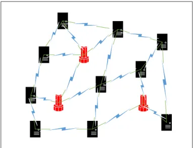
Figure 1.1: Interconnected physical machines and sink nodes in an unstructured network topology.
As illustrated in Figure 1.1, assuming a general unstructured network
topology, some small number of nodes (shown as cylinder-shaped components) are functionally different than the rest. With a high probability, any VM to be placed in the ordinary PMs will be somehow dependent on at least one of the sink nodes shown in the figure. By dependence, we mean the tendency to require massive end-to-end traffic between a given VM and a sink that the VM is dependent on. With that definition, the intenser the requirement is, the more dependent the VM is said to be.
The network connecting the nodes can be represented as a general graph G(V, E) where E is the set of links and V is the set of nodes (including PMs and sinks as shown in relation 1.1). On the other hand, the number of normal PMs
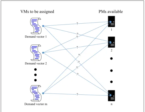
is much larger than the number of sinks (relation 1.2): S ∈ V (1.1) |S| |V − S| (1.2) 1 2 3 Sinks VMs to be placed Demand Vector 1 Demand Vector 2 Demand Vector m
Figure 1.2: The dependence of any VM on any sink given as demand vector. Each link consisting of end nodes ui and uj is associated with a capacity cij
that is the maximum flow that can be transmitted through the link.
Assume that the intensity of communication between physical machines is negligible compared to the intensity of communication between physical machines and sinks. In such a scenario, it makes sense to assume that the quality of communication (in terms of delay, flow, etc.) between VMs and the sinks is the most important factor that we should focus on. That is, placing the VMs on PMs that offer a better quality according to the demands of the VMs, is a reasonable decision. Before advancing further, we suppose that the following prior information is given about any VM:
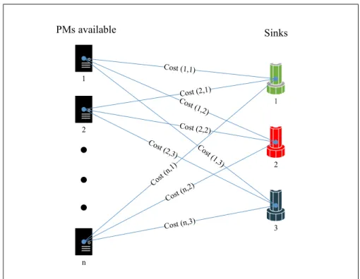
1 2 n PMs available 1 2 3 Sinks
Figure 1.3: The costs between any PM-Sink pair.
• Total Flow: The total flow that the VM will demand in order to send to and/or receive data from sinks.
• Demand Weight: For a particular VM (vmi), the weights of the demands for
the sinks are given as a demand vector Vi = (vi1, vi2, . . . , vi|S|) with elements
between 0 and 1 whose sum is equal to 1. (vik is the weight of demand for
sink k in vmi). Figure 1.2 illustrates what demand vector means.
Suppose that each PM-Sink pair is associated with a numerical cost as depicted in Figure 1.3 (to be explained in detail later). It is clearly not a good idea to place a VM with intensive demand for sink x in a PM that has a high cost associated with that sink.
Based on those assumptions, we define a metric named satisfaction that shows how “satisfied” a given virtual machine v is, when placed on a physical machine p.
1 2 n Demand vector 1 Demand vector 2 Demand vector m VMs to be assigned PMs available
Figure 1.4: The Placement Problem that can be represented as an Assignment Problem that maps VMs to PMs.
the service provider and the service consumer side will be in a win-win situation. From consumer’s point of view, the VMs will experience a better quality of service. Similarly, on the provider side, the links will be less likely to be saturated which enables serving more VMs.
The placement problem (Figure 1.4) in our scenario is the complement of the famous Quadratic Assignment Problem (QAP) [36] which is NP-hard. On account of the dynamic nature of the VMs that are frequently commenced and terminated, it is impossible to arrange the sinks optimally in a constant basis, since it requires physical changes in the topology. So, we instead attempt to find optimal placement (or actually nearly-optimal placement) for the VMs which is exactly the complement of the aforementioned problem. We propose greedy and heuristic based approaches that show different behavior according to the topology (Tree, VL2, etc.) of the network.
We introduce two different approaches for the placement problem including a greedy algorithm and a heuristic-based algorithm. Each of these algorithms
have two different variants. We test the effectiveness of the proposed algorithms through simulation experiments. The results reveal that a closer to optimal placement can be achieved by deploying the algorithms instead of assigning them regardless of their needs (random assignment). We also provide a comparison between the variants of the algorithms and test them under different topology and problem size conditions.
The rest of this thesis includes a brief background about cloud computing together with literature review (Chapter 2) followed by the formal definition of the problem in hand (Chapter 3). In Chapter 4, some algorithms for solving the problem are provided. Experimental results and evaluations are included in Chapter 5. Finally Chapter 6 concludes the thesis and proposes some potential future work.
Chapter 2
Background
2.1
Cloud Computing
Nowadays, Cloud Computing is becoming a famous buzzword. As a brand new infrastructure to offer services, Cloud Computing systems have many superiorities in comparing to those existed traditional service provisions, such as reduced upfront investment, expected performance, high availability, infinite scalability, tremendous fault-tolerance capability and so on, and consequently chased by most of the IT companies, such as Google, Amazon, Microsoft, Salesforce.com [14]. Cloud Computing provides a paradigm shift following the shift from mainframe to client–server architecture in the early 1980s [9, 12] and rather than a product, in this novel paradigm computing is delivered as a service. In such a paradigm, resources, software, or information are services that are provided to customers over networks.
Cloud Computing refers to both the applications delivered as services over the Internet and the hardware and systems software in the data centers that provide those services [16].
Nevertheless, there are quite a few different definitions for Cloud Computing
Computing is not a completely novel concept as it is conceptually connected to some relatively new paradigms such as Grid Computing, utility computing, cluster computing, and distributed systems in general. [24].
2.1.1
Hardware Virtualization
Literally, hardware virtualization means that an application executes on virtualized hardware as opposed to physical hardware [15]. Virtualization is a technology that draws a separation line between computation and physical
hardware. This technology is often referred to as the groundwork for Cloud
Computing for its ability to isolate software from hardware, and in turn isolating users and processes/resources. Traditional operating systems are not capable of providing such degree of isolation that suits well for Cloud Computing. Hardware virtualization approaches include Full Virtualization, Partial virtualization and Paravirtualization [17]. With virtualization, software capable of execution on the raw hardware can be run in a virtual machine. Cloud systems deployable services can be encapsulated in virtual appliances (VAs) [18], and deployed by instantiating virtual machines with their virtual appliances [19].
In [15] Plessl and Platzner compare the three different approaches of hardware virtualization arguing the motives behind each approach:
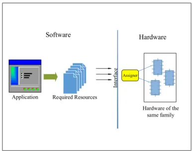
• Temporal Partitioning: Partially deployed but insufficient resources may be sequentially utilized to run a specific splittable application. Temporal Partitioning maps an application of arbitrary size to a device with insufficient resources having the reconfigurability feature (Figure 2.1). • Virtualized Execution: Virtualized execution is meant to achieve a certain
level of device-independence within a device family. An application is mapped to or specified directly in a programming model (Figure 2.2). • Virtual Machine: The motivation for this virtualization approach is to
achieve an even higher level of device-independence. Instead of mapping an application directly to a specific architecture, the application is mapped
Application S eque nti al F ee de r Output Aggregator Insufficient Resource Application Partitions
Figure 2.1: Temporal Partitioning.
to an abstract computing architecture. Java Virtual Machine [25, 26]
is probably the most renown example of this virtualization category (Figure 2.3).
2.1.2
The XaaS Service Models
There are several service models that are related to cloud computing out of which some are very important and they are worthy to be mentioned here. Furthermore, these services fill into three levels: hardware level, system level and application level [14].
• Software as a Service (SaaS): In this model, software applications are the actual services that are executed on infrastructures that are managed by a vendor. Customers often use certain family of clients such as web browsers and programming interfaces to access the provided services. Normally, users are charged on a subscription basis [20]. Customers have often no idea of the working mechanisms in the underlying infrastructure where their applications are serviced. In other words, there is a level of transparency between customers and the infrastructure.
Application Inte rf ac e Hardware Software Required Resources Hardware of the same family Assigner
Figure 2.2: Virtualized Execution.
• Platform as a Service (PaaS): In the PaaS model, computing platform or solution stack normally consisting of operating system, programming language IDE, database, and web server are delivered as services to consumers [21]. Without a necessity to oversee and control the bottom layer of software and hardware (e.g. Network, OS, physical data storage) users or customers can simply develop and run their software and also manage their applications (e.g. configuration settings for the hosting environment) if required [22].
• Network as a Service (NaaS): Examples of the services that fall into NaaS category abound. Amongst, there are some popular ones such as Internet services from carriers (both wired and wireless network service), mobile
services and alike. The Internet services are mainly concerned with
providing broadband bandwidth-on-demand services [14].
• Data as a Service (DaaS): The DaaS refers to the family of services provided by means of software as a service or web service that offer access and analytics to a set of proprietary set of aggregated data. Several renown companies such as DataDirect [27] and Strikeiron [28] are providing that service to customers.
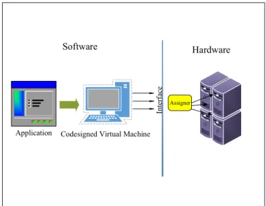
Application Codesigned Virtual Machine Inte rf ac e Hardware Software Assigner
Figure 2.3: Virtual Machine.
hardware resources including components like storage capacity, memory, CPU cycles, and Network facilities are called infrastructure. IaaS is a service model in which infrastructure is delivered as service, typically over the Internet. Some popular companies with huge investments on hardware that offer such services include Amazon [29], ServePath [30], Mosso [31], and Skytap [32]. Those services often charge in terms of customer usage [14]. In this model, the customers have more flexibility as they are able to run their desired software that can be ordinary applications or even operating systems. Nevertheless, the underlying cloud infrastructure is not under direct control of the users. Customers can only manipulate and control their own virtual infrastructure that is formed by virtual machines hosted by physical IaaS vendors. In this thesis, although we are not confined to a particular service model, we will mostly focus on infrastructure as a service model.
2.1.3
Cloud Computing Scenarios
Regardless of the service model that is used, one can think of two major stakeholders: 1- Infrastructure Provider (IP), and 2- Service Provider (SP). The
first refers to the party that offers infrastructure and resources such as data centers, storage capacities, networks, etc, while the latter refers to the party that delivers the services provided by the IP to the end users. The provided services can be of any family (e.g. SaaS, NaaS, ...) that in most cases are deployed using PaaS tools. According to [23], cloud scenarios can be roughly classified into four categories:
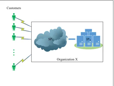
• Private Cloud: In such a scenario, the SP and IP are integrated as a single provider and the corresponding organization provisions services depending on its own internal infrastructure. One obvious advantage of this scheme is the lack of transparency between the IP and SP enabling a better control and higher performance as the whole cloud is administered within a united
capsule. Higher security can be counted as another advantage of the
mentioned scenario. Figure 2.4 provides a graphical illustration of private cloud scheme.
SPX
Organization X Customers
IPX
Figure 2.4: Private Cloud Scheme.
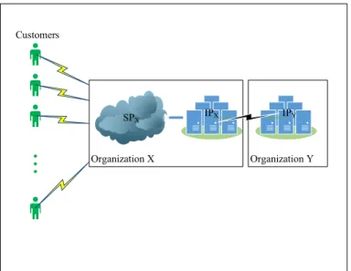
• Cloud Bursting: Figure 2.5 depicts a different scenario where one or more IPs are deployed as backup Infrastructure Providers along with a local one. In some unavoidable situations, the local IP may not be capable of handling the demands due to a burst workload and/or it might be facing periodical failures. The usage of multiple back up IPs guarantees that the scheduled
jobs can be offloaded to a different IP in any unpredicted or anomalous circumstance. SPX Organization X Organization Y IPX IPY Customers
Figure 2.5: Cloud Bursting Scheme.
• Federated Cloud: According to [33], a federated cloud (Figure 2.6) is a collection of a Service Provider and multiple collaborative Infrastructure Providers that try to balance the load between themselves. The federation is often transparently associated with the IP level and SP has no control over it. Put differently, an SP that assigns a job to an IP in a federation, is not aware of the fact that the job might be/have been offloaded to a different IP for load balancing purposes. Nonetheless, the SP is sometimes able to enforce location constraints on the service (e.g. by requiring it to be provisioned in particular IP(s)).
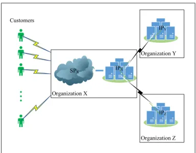
• Multi-Cloud: A federated cloud without transparency between the SP and IPs is equivalent to Multi-Cloud scenario. As shown in Figure 2.7, in such scenarios, the SP is responsible for coordinating the IPs and deal with load balancing and optimality challenges. We can think of a similarly defined special case scenario where the organization has no internal IP and depends totally on the external ones. In this case as the SP depends totally on external infrastructures, cost-related optimization problems often draw attention.
Organization Y IPY Organization Z IPZ SPX Organization X IPX Customers
Figure 2.6: Federated Cloud Scheme.
2.2
Service Assignment Problems
Simply put, the Cloud assignment problems are related to finding an optimal solution for determining how to map a set of requested services to a set of local or in some cases remote resources. The requested services may consist of several components whose assignment should be considered separately. Moreover, the scenario and service model is also important in deciding where to assign a given demand. The characteristics of the demands also are dependent upon the service model and scenario. In the following subsections, a brief introduction to some factors and criteria as well as challenges when dealing assignment problems are given.
2.2.1
Parameters and Criteria
Numerous factors and parameters including (but not limited to) Data Center capacities, network constraints, pricing, locality, etc. should be taken into account when designing an effective assignment algorithm. Otherwise, the output can be unsatisfactory or it can yield contradictory outcomes for different stakeholders. The assignment algorithm should be intricately designed to honor the advantages
Organization Y IPY Organization Z IPZ SPX Organization X IPX Customers
Figure 2.7: Multi-Cloud Scheme.
of the stakeholder (IP or SP) that it is meant to be associated with. That being the case, typically there is a price-performance trade-off intrinsic to assignment problems in Cloud systems that should be alleviated. Below, some of the most important factors that are mostly used as criteria for evaluating an assignment algorithm are given.
• Performance: Virtualization and consolidation are the most popular
techniques to enhance the utilization of physical resources such as data centers and network bandwidth enabling the server platforms to run possibly heterogeneous applications. However, the significance of placement algorithms are coequally essential meaning that deploying different VM placement strategy can affect the performance substantially in an unvarying scenario [34].
• Cost: Although fixed schemes used to be dominant for modelling Cloud
prices in the infancy days of Cloud technology, it has gradually shifted to the dynamic pricing schemes [35]. Without any undesired impact on the performance of a given service, it is possible to diminish the investment amounts by reconfiguring the services dynamically [37]. One example of this reconfiguration is resizing VMs without any disadvantageous consequences. Besides, the reciprocal competitive effect of VMs (e.g. intervention and
rivalry of different VMs trying to access the same resource such as CPU cycles) should also be taken into consideration when modelling the price for a Cloud service.
• Reliability and Availability of the Services: In some scenarios, objective VM placement objective is guaranteeing a reliable service with highest possible availability being cognizant of resource constraints. Several techniques can be applied to achieve such goals including replication and migration of VMs across diverse physical machines possibly located in remote geographical zones. A higher level of reliability and availability depends on the reliability of hosting data centers, the significance of service and any associated data that is enclosed in VMs, the access frequency are the most important factors that one should bear in mind when designing a VM placement algorithm for maximizing the reliability and availability of the service [45].
• Locality: Locality is a beneficial quality unless some other more vital factors in stake such as security are conflictingly affected [43]. The closeness of a VM (or service) to its corresponding user is referred to as locality [42]. Maximizing this factor is specifically related to metrics such as congestion in the deployed networks. Our thesis is closely tied to VM placement in a scenario that locality should be highlighted in order to achieve a better performance in the underlying physical network.
2.2.2
Challenges
Developing a general-purpose placement mechanism is infeasible due to the magnitude of different scenarios, the range of parameters, conflict of different
stakeholders’ interests, etc. Below, some of the challenges that make the
placement problem even more demanding are listed.
• To begin with, in some situations it is very difficult to model the requirements of the users when there is no defined prototype model that reflects the exact
needs and all the thresholds for the users. In other words, the ever changing service models and scenarios may be evolving too fast to catch up with and adapt the placement method accordingly.
• Moreover, it is often a very taxing job to find proper parameters when trying to do model parameterization especially when the size of the problem is too large.
• Last but not least, the VM placement problems can often be reduced to well-known NP-hard problems such as multiple-knapsack [4]. Therefore, finding a perfect solution that can be run in a reasonable amount of time specially in online problems with huge size is almost impossible (e.g., Amazon EC2 [29], the leading cloud provider, has approximately 40,000
servers and schedules 80,000 VMs every day [44]). The solution is to
use approximation algorithms and heuristic-based approaches to be able to achieve an acceptable result in a practicable time.
2.3
The Scope of This Thesis
Considering the complexity and variety of Virtual Machine placement problems, the subject and/or scenario orientedness of any proposed placement algorithm is something inevitable. That being said, the placement problem studied in this thesis is also limited to a specific scenario and assumes the availability of some apriori knowledge such as VM bandwidth demand profile information. In this work, we are concerned with optimal usage of network resources rather than any other Cloud assets including physical machines, or even some microscopic level resources like CPU cycles, memories, storage capacities and alike. The constraints that we consider in developing our VM placement algorithm are also related to the underlying network infrastructure that is deployed as a part of Cloud. We propose off-line VM placement approaches having a reasonable time complexity and yielding near optimal results.
2.4
Related Work
There are several studies in the literature that are closely related to our work. In [46] consolidation has been viewed from a different angle: consolidation is primarily meant to require VMs be packed tightly while they also receive resources commensurate with their demands. However, network bandwidth demands of VMs may be too dynamic that will make it difficult to distinguish demands by a fixed number and try to apply conventional consolidation schemes. In their work, they capture the bandwidth demand by random variables obeying probabilistic distributions. The mentioned study is focused on consolidating VMs according to bandwidth constraints enforced by network devices including Ethernet adapters and edge switches. They formulate the problem as a Stochastic Bin Packing problem and then propose an online packing algorithm.
In a different work [47] carried out by O. Biran et al. focused on Virtual Machine placement problem, researchers contend that placement has to carefully consider the aggregated resource consumption of co-located VMs in order to be able to honor Service Level Agreements (SLA) by spending the least or
comparatively fewer costs. In their work, they focus on both network and
CPU-memory requirements of the VMs. Their proposed methods that not only satisfies the anticipated communication demands of the VMs, but is also resilient to variations happening over time.
The scalability of data centers have been carefully studied by X. Meng et al. in their work [48]. They propose a traffic-aware Virtual Machine placement to improve the network scalability. Unlike past works, their proposed methods do not require any alterations in the network architecture and routing protocols. They suggest that traffic patterns among VMs can be better matched with the communication distance between them. They formulate the VM placement as an optimization problem and then prove its hardness. In the mentioned work, a two-tier approximate algorithm is proposed that solves the VM placement problem efficiently.
research [49] followed through with D. Breitgand and A. Epstein. They suggest that consolidating VMs should be realized without quality of service degradation. The study is related to the problem of consolidating VMs on the minimum number of containers interconnected using a network where there is a bottleneck possibility.
To the best of our knowledge the most relevant past work is [50] by R. Cohen et al. In their work, they concentrate merely on the networking aspects and consider the placement problem of virtual machines with intense bandwidth requirements. They focus on maximizing the benefit from the overall communication sent by virtual machines to a single point in the data center which they call root. In a storage area network of applications with intense storage requirements, the scenario that is described in their work is very likely. They propose an algorithm and simulate on different widely used data center network topologies.
There are some less related works that also focus on network aspects of cloud computing but from different standpoints such as routing, scalability, connectivity, load balancing and alike:
In [38], M. Al-Fares et al. argue that the aggregate bandwidth requirements of an immense number of computers that are contained in a data center network can be huge. The typical infrastructure of the utilized networks consists of tree of routing and switching elements with progressively more specialized and expensive components moving upwards in the network hierarchy. Their work contends that this architecture after even deploying the higher-end IP switches or routers may only support half of the aggregate bandwidth available at the edge of the network. They try to interconnect the commodity switches in different ways to deliver more performance at less cost than available from popular higher-end solutions. Their approach does not require any alterations on the end host network interface, OS, and applications.
A network architecture is proposed by [39] by A. Greenberg et al. to allow dynamic resource allocation across large server pools. They declare that the data center network should allow any server to be assigned to any service, and VL2 meets that requirement. They have also made a real working prototype of VL2.
Similarly, in [40], C. Guo et al. propose a network architecture named BCube that is specifically aimed for shipping-container based and modular data centers. In this architecture, servers with multiple network ports connect to multiple layers of COTS (commodity the-shelf) mini-switches, relaying packets to other servers which is against what happens in other architectures where servers are only end hosts. According to their experiments, among the most important features of BCube is accelerating bandwidth intensive applications.
Finally, in [41] a study of application demands from a production data center of 1500 servers by S. Kandula et al. reveals that in many cases application demands can be generally met by a network that is slightly oversubscribed. In their work, they advocate a hybrid architecture claiming that eliminating over-subscription is a needless overkill. In their approach, after the base network is provisioned for the average case, for the hotspots they add extra links on
an on-demand basis. The additional links are called flyways that provide
Chapter 3
Formal Problem Definition
We are interested in the problem of finding an optimal assignment of a set of Virtual Machines (VMs) into a set of Physical Machines (PMs) (assuming that the number of PMs is greater than or at least equal to that of VMs) in a special scenario with the objective of maximizing a metric that we define as satisfaction. In the following sections, the scenario of interest, assumptions, the defined metric, and mathematical description of the problem are provided, respectively.
3.1
Scenario
Heterogeneity of interconnected physical resources in terms of computational power and/or functionality is not too unlikely in Cloud Computing environments [52]. If we refer to any server (or any connection point) in Data Center Network (DCN) as a node, assuming that the nodes can have different importance levels is also reasonable in some situations. Note that here, since we are concerned with network constraints and aspects, by importance level we mean the intensity of traffic that is expected to be destined for a subject node. In other words, if VMs have a higher tendency to initiate traffics to be received and processed by a certain set of nodes (call it S), we will say that the nodes belonging to that set have a higher importance (e.g., the cylinder-shaped servers shown in Figure 1.1).
Throughout the thesis, those special nodes are called sinks. Besides, a sink can be a physical resource such as a supercomputer or it can be a virtual non-processing unit such as a connection point:
One can think of a sink as a physical resource (as is the case in Figure 1.1) that other components are heavily dependent on. A powerful supercomputer capable of executing quadrillions of calculations per second [53] can be considered a physical resource of high importance from network’s point of view. Such resources can also be functionally different from each other. While a particular server X is meant to process visual information, server Y might be used as a data encrypter. In our scenario, a sink is not necessarily a processing unit or physical resource. It can also be a connection point to other clouds located in different regions meant for variety of purposes including but not limited to replication (Figure 3.1). Suppose that in the mentioned scenario, every VM is somehow dependent on those sinks in that sense that there exists reciprocally intensive traffic transmission requirement between any VM-sink pair.
Cloud in Region 1 Cloud in Region 2
Cloud in Region 3 Cloud in Region 4
Local Cloud
Connection Point Resource Link
Figure 3.1: Non-resource Sinks.
Regardless of the types of the sinks (resource or non-resource) the overall traffic request destined for them is assumed to be very intense. Having said that, functional differences might exist between the sinks that can in turn result in a disparity on the VM demands. We assume that any VM has a specific demand
weight for any given sink.
In the subject scenario, the tendency to transmit unidirectional and/or bidirectional massive traffic to sinks is so high that it is the decisive factor in measuring a VM’s efficiency. Also, Service Level Agreement (SLA) requirements are satisfied more suitably if all the VMs have the best possible communication quality (in terms of bandwidth, delay, etc.) with the sinks commensurate to their per sink demands. For example, in Table 3.1 three virtual machines are given associated with their demands for each sink in the network. An appropriate placement must honor the needs of the VMs by placing any VM as close as possible to the sinks that they tend to communicate with more intensively (e.g., require a tenser flow).
Table 3.1: Sink demands of three VMs.
VM/Sink S1 S2 S3
VM1 0.1 0.2 0.7
VM2 0.5 0.05 0.45
VM3 0.8 0.18 0.02
3.2
Assumptions
The scenario explained in Section 3.1 is dependent upon several assumptions that are explained below:
• Negligible Inter-VM Traffic: The core presupposition that our scenario is based on, is assuming that the sinks play a significant role as virtual or real resources that VMs in hand attempt to acquire as much as possible. Access to the resources is limited by the network constraints and from a virtual machine’s point of view, proximity of its host PM (in terms of cost) to the sinks of its interest matters the most. Therefore, we implicitly make an assumption on the negligibility of inter-VM dependency meaning that VMs
do not require to exchange very huge amounts of data between themselves. If we denote the amount of flow that VM vmidemands for sink sj by D(i, j),
and similarly denote the amount of flow that VM vmkdemands for another
VM vml by D0(k, l), then Relation 3.1 must hold where i, j, k, and l are
possible values (i.e., i ≤ number of VMs, and j ≤ number of sinks):
D0(k, l) D(i, j), ∀i, j, k, l (3.1)
• Availability of VM Profiles: Whether by means of long term runs or by
analyzing the requirements of VMs at the coding level, we assume that the sink demands of the VMs based on which the placement algorithms operate are given. In other words, associated with any VM to be placed, is a vector called demand vector that has as many entries as the number of sinks (Figure 3.2). Virtual Machine X 0.2 0.15 0.2 0.05 0.1 0.2 0.1 Demand Vector X VM Request X Total Sink Flow Demand for X
Figure 3.2: Incoming VM Request.
Suppose that the sinks are numbered and each entry on any demand vector corresponds to the sink whose number is equal to the index of the entry. Entries in the demand vectors are the indicators of relative importance of corresponding sinks. The value of each entry is a real value in the range [0,1] and the summation of entries in any demand vector is equal to 1. In addition to demand vector, we suppose that a priori knowledge about the
total sink flow demand of any VM is also given. Sink flow demand for a particular VM vmx is defined as the total amount of flow that vmx will
exchange with the sinks cumulatively.
• Off-line Placement: The placement algorithms that we propose are off-line meaning that given the information about the VMs and their requirements, network topology, physical machines, sinks, and links, the placement happens all in once as shown in Figure 3.3.
VM Requests
Network Topology, Physical Resources, Sinks, and Link
Information
Input
Final Assignment Table Mapping VMs to PMs VM to PM
assigner Algorithm
Algorithm Output
Figure 3.3: Off-line Virtual Machine Placement.
• One VM per a PM: We suppose that every PM can accommodate only one VM. Although this assumption may sound unrealistic, it is always possible to consolidate several VMs as a single VM [50]. In a real world scenarios, CPU and memory capacity limits of each host determines the number of VMs that it can accommodate. A different approach is to is to bundle all VMs that can be placed in a single host into one logical VM, with the accumulated bandwidth requirements. In both cases we can thus assume with the loss of generality throughout the thesis that each PM can accommodate a single VM.
3.3
Satisfaction Metric
The placement problem in our scenario can be viewed from two different stakeholders’ perspective: From a Service Provider’s standpoint, an appropriate placement is the one that honors the virtual machines’ demand vectors. Comparably, Infrastructure Provider tries to maximize the locality of the traffics and minimize the flow collisions. Fortunately, in our scenario, the desirability of a particular placement from both IP and SP viewpoints are in accordance: any placement mechanism that respects the requirements of the VMs (their sink demands basically), also provides more locality and less congestion in the IP side. We define a metric that shows how satisfied a given VM vmi becomes when it
is placed on PM pmj. In our scenario, satisfaction of a virtual machine depends
on the appropriateness of the PM that it is placed on according to its demand vector. As it is illustrated on Figure 1.3, there is a cost associated between any PM-Sink pair. Likewise, there is a demand between any VM-Sink pair that shows how important a given sink for a VM is (Figure 1.2). A proper placement should take into account the proximity of VMs to the sinks proportionate to their significance. Here, by proximity we mean the inverse of cost between a PM and a sink: a lower cost means a higher proximity. As an example, suppose that we have one VM and two options to choose from (Figure 3.4): pm1 or pm2.
In this example, there are three sinks in the whole network. The VM is given together with its total flow demand and demand vector. The costs between pm1
and all the other sinks supports the suitability of that PM to accommodate the given VM because more important sinks have a smaller cost for pm1. Sinks 3, 2
and 1 with corresponding significance values 0.7, 0.25, 0.05 are the most important sinks, respectively. The cost between pm1 and sink 3 is the least among the three
cost values between that PM and the sinks. The next smallest costs are coupled with sink 2 and sink 1, respectively. If we compare those values with the ones between pm2 and the sinks, we can easily decide that pm1 is more suitable to
accommodate the requested VM. If we sum up the values resulted by dividing the value of each sink in the demand vector of a VM to the cost value associated with that sink in any potential PM, then we can come up with a numerical value
Virtual Machine pm1 pm2 Sink 1 Sink 2 Sink 3 2 Sink 1 Sink 2 Sink 3 1 0.7 0.25 0.05
Figure 3.4: A simple example of placement decision.
reflecting the desirability of that PM to accommodate our VM. For now, let’s denote this value by x(vm, pm) which means the desirability of physical machine pm for virtual machine vm. The desirability of pm1 and pm2 for the given VM
request in our example can be calculated as follows (Equations 3.2 and 3.3):
x(vm, pm1) = 0.05 5 + 0.25 2 + 0.7 1 = 0.835 (3.2) x(vm, pm2) = 0.05 2 + 0.25 1 + 0.7 5 = 0.415 (3.3)
From these calculations, it is clearly understandable that placing the requested VM on pm1 will satisfy the demands of that VM in a better manner.
Based on that intuition, given a VM vm with demand vector V including entries v1, ..., v|S|, a set of PMs P = {pm1, ..., pm|P |}, the set of sinks S =
{s1, ..., s|S|}, a static cost table D with entries Dij indicating the static cost
between pmi and sj, and a dynamic cost function G(pm, s, vm) that returns the
the satisf action function Sat(vm, pm) as: Sat(vm, pmi) = |S| X j=1 vj dij × G(pmi, sj, vm) (3.4)
The details of D table and G function in Relation 3.4 are provided in the next section (Mathematical Description). Note that for the sake of simplicity but without the loss of generality, we assume that the static costs are as important as the dynamic costs in our scenario (i.e., according to the Relation 3.4, a PM p with static cost cs and dynamic cost cdassociated with a sink s is as desirable as
another PM p0 with static cost c0s = 12.cs and dynamic cost c0d = 2.cd associated
with s, for any VM that has an intensive demand for s). Static and dynamic costs are of different natures and their combined effect must be calculated by a precisely parameterized formula that depends on the sensitivity of the VMs to delay, congestion, and so on.
3.4
Mathematical Description
The problem in hand can be represented in mathematical language. First of all, topology of the network is representable as a graph G(V, E) where V is the set of all resources (including PMs and sinks) and E is the set of links (associated with some values such as capacity) between the resources (Figure 3.5). In addition to the topology, we have the following information in hand:
• Set N = pm1, pm2, . . . , pmn consisting of physical machines.
• Set M = vm1, vm2, . . . , vmm consisting of virtual machine requests.
where Relations 3.5 and 3.6 hold: |N | ≥ |M | (3.5) |N | |S| (3.6) D E C A B 7 23 22 21 20 18 19 16 17 15 13 10 9 8 6 3 12 5 2 1 4 11 14 F
Figure 3.5: A graph representing a simple data center network without an standard topology. The nodes named by alphabetic letters are the sinks.
In addition, any VM request has a sink demand vector and a total sink flow:
• fi = total sink flow demand of vmi. In other words, it is a number that specifies
the amount of demanded total flow for vmi that is destined for the sinks.
• Vi = (vi1, vi2, . . . , vi|S|) which is the demand vector for vmi. In this vector,
For any demand vector, we have the following relations (3.7 and 3.8): |S| X j=1 vij = 1, ∀i (3.7) 0 ≤ vij ≤ 1, ∀i, j (3.8)
All of the resources in the graph G can be separated into two groups, namely, normal physical machines and sinks (that can be special physical machines or virtual resources like connection points as explained in Section 3.1). With that in mind, as illustrated in Figure 3.6, we can think of a bipartite graph Gp = (N ∪ S, Ep) whose: 2 3 4 5 6 23 F D E C A B 1
Figure 3.6: A bipartite graph version of Figure 3.5 representing the costs between PMs and sinks.
• Vertices are the union of physical machines and sinks.
The cost associated with any PM-Sink pair is in direct relationship with static costs such as physical distance (e.g., it can be the number of hops or any other measure) and dynamic costs such as congestion as a result of link capacity saturation and flow collisions. It means that depending on different assignments, the cost value on the edges connecting the physical machines to the sinks can also change. For example, according to Figures 3.5 and 3.6, if a new virtual machine is placed on PM #18 that has a very high demand for the sink C, then the cost between PM #23 and the sink C will also change most likely. Suppose that PM #23 uses two paths to transmit its traffic to sink C: P1 = {22 − 21 − 18} and
P2 = {22 − 20 − 19} (excluding the source and destination). Placing a VM with
an extremely high demand for sink C on 18 can cause a bottleneck in the link connecting 18 to the mentioned sink. As a result, PM #23 may have a higher cost for sink C afterwards, since the congested link is on P1 which is used by PM
#23 to send some of its traffic through. Accordingly, we define:
• D Matrix : A matrix representing the static costs between any PM-Sink pair which is an equivalent of the example bipartite graph shown in Figure 3.6 in its general case. An entry Dij stores the static cost between pmi and sj.
• G Function: For any VM, the desirability of a PM is decided not only according to static but also dynamic costs. G(pmi, sj, vmk): N × S × M →
R+ = congestion function that returns a positive real number giving a sense
of how much congestion affects the desirability of pmi when vmk is going
to be placed on it, taking into account the past placements. Congestion happens only when links are not capable of handling the flow demands perfectly. The G function returns a number greater than or equal to 1 which shows how well the links between a PM-Sink pair are capable of handling the flow demands of a particular VM. If the value returned by this function is 1, it means that the path(s) connecting the given PM-Sink pair won’t suffer from congestion if the given VM is placed on the corresponding PM. Because the value returned by G is a cost, a higher number means a worse condition. Implicitly, G is also a function of past placements that dictate how network resources are occupied according to the demands of the VMs. While there is no universal algorithm for G function as its output is
totally dependent on the underlying routing algorithm that is used, it can be described abstractly as shown in Figure 3.7. According to that figure, the G function has four inputs out of which two of them are related to the assignment that is going to take place (VM Request and PM-Sink pair) and the rest are related to past assignments and their effects on the network (the occupation of link capacity and so on).
Network Topology, Link Information Input Output Past Assignments VM Request Does Congestion Affect the Cost Between the PM and
Sink Pair? PM-Sink Pair G Function (abstract view) 1 N Y (Flow)
Figure 3.7: The abstract working mechanism of G function.
Based on the underlying routing algorithm used, the inner mechanism of G function can be one of the followings:
• Oblivious routing with single shortest path: For such a routing
scheme, the G function simply finds the most occupied link and divides the total requested flow over the capacity of the link (refer to Algorithm 1). If the value is less than or equal to 1, then it returns 1. Otherwise, it returns the value itself. According to Figure 3.8, physical machines X and Y use static paths (1-2-3 and 1-2-4, respectively) to send their traffic to the sink. Suppose that among the links connecting X to the sink, only the link 1-2 is shared with a different physical machine (Y in that case). Link 1-2 is therefore the most occupied link and if we call the G function for a given VM, knowing that another VM
is placed on Y beforehand, according to the demands of the previously placed VM and the VM that is going to be assigned to Y , G will return a value greater than or equal to 1 showing the capability of the bottleneck link of handling the total requested flow.
Algorithm 1 G(pmi, sj, vmk) : The congestion function for oblivious routing
with single path.
1: Path ← the path connecting pmi and sj
2: MinLink ← the link in the Path that is occupied the most
3: totReq ← total flow request destined to pass through MinLink
4: c ← Total Capacity of MinLink
5: G = totReqc
6: return max(G, 1)
Figure 3.8: A partial graph representing part of a data center network. The colored node represents a sink. Physical machines X and Y use oblivious routing to transmit traffic to the sink. The thickest edge (1-2) is the shared link.
• Oblivious routing with multiple shortest (or acceptable) paths: If there are more than one static path between the PM-Sink pairs and the load is equally divided between them, then the G function can be defined in a similar way with some differences: every path will have its own bottleneck link and the G function must return the sum
of requested over total capacity of the bottleneck links in every path divided by the number of paths (Algorithm 2). Hence, if congestion happens in a single path, the overall congestion will be worsened less than the single path case. In Figure 3.9, two different static paths (1-2-3, 6-7-8-9 for X, and 5-4, 1-7-8-9 for Y) have been assigned to each of the physical machines X and Y. The total flow is divided between those two paths and the congestion that happens in the links that are colored green, affects only one path of each PM.
Algorithm 2 G(pmi, sj, vmk) : The congestion function for oblivious routing
with multiple paths.
1: n ← number of paths connecting pmi to sinkj
2: TotG ← 0
3: for all Path between pmi and sinkj do
4: MinLink ← the link in the Path that is occupied the most
5: totReq ← total flow request passing from MinLink
6: c ← Total Capacity of MinLink
7: G = totReqc
8: TotG ← TotG + G
9: end for
10: return max(T otGn , 1)
• Dynamic routing: Defining a G function for dynamic routing is more
complex and many factors such as load balancing should be taken into account. However, the heuristic that we provide for placement, is independent from the routing protocol. G functions provided for oblivious routing can be applied to two famous topologies, namely Tree and VL2 [39].
We are now ready to give a formal definition of the assignment problem. The problem can be formalized as a 0-1 programming problem, but before we can advance further, another matrix must be defined for storing the assignments:
• X matrix: X : M × N → {0, 1} is a two dimensional table to denote
Figure 3.9: The same partial graph as shown in Figure 3.8, this time with a multi-path oblivious routing. Physical machines X and Y use two different static routes to transmit traffic to the sink. The thicker edges (7-8, 8-9, and 9-sink) are the shared links. The paths for X and Y are shown by light (brown) and dark (black) closed curves, respectively.
The maximization problem given below (3.9) is a formal representation of the problem in hand as an integer (0-1) programming. Given an assignment matrix X, VM requests, topology, PMs, sinks and link related information the challenge is to fill the entries of the matrix X with 0s and 1s so that it maximizes the objective function and does not violate any constraint.
M aximize |M | X i=1 |N | X j=1 Sat(vmi, pmj).xij (3.9) Sat(vmi, pmj) = |S| X k=1 vik djk × G(pmj, sk, vmi) Such that |M | X xij = 1, for all j = 1, ..., |N | (1)
|N |
X
j=1
xij = 1, for all i = 1, ..., |M | (2)
xij ∈ {0, 1}, for all possible values of i and j (3)
The constraints (1) and (2) ensure that each VM is assigned to exactly one PM and vice versa. Constraint (3) prohibits partial assignments. As explained before, function G gives a sense of how congestion will affect the cost between pmj and sk if vmi is about to be assigned to pmj.
We can represent the assignment problem as a bipartite graph that maps VMs into PMs. The edges connecting VMs to PMs are associated with weights which are the satisfaction of each VM when assigned to the corresponding PM. The weights may change as new VMs are placed in the PMs. It depends on the capacity of the links and amount of flow that each VM demands. Therefore, the weights on the mentioned bipartite graph may be dynamic if dynamic costs affect the decisions. If so, after finalizing an assignment, the weights of other edges may require alteration. Because congestion is in direct relationship with number of VMs placed, after any assignment we expect a non-decreasing congestion in the network. However, the amount of increase can vary by placing a given VM in different PMs. According to the capacity of the links, we expect to encounter two situations:
3.4.1
First Case: No congestion
If the capacity of the links are high enough that no congestion happens in the network, the assignment problem can be considered as a linear assignment problem which looks like the following integer linear programming problem [54]. Given two sets, A and T (assignees and tasks), of equal size, together with a weight function C : A × T → R. Find a bijection f : A → T such that the cost
function P
a∈AC(a, f (a)) is minimized:
M inimizeX i∈A X j∈T C(i, j).xij (3.10) Such that X i∈A xij = 1, for i ∈ A X j∈T xij = 1, for j ∈ T
xij ∈ {0, 1}, for all possible values of i and j
In that case, the only factor that affects the satisfaction of a VM is static cost which is distance. The assignment problem can be easily solved by Hungarian Algorithm [54] by converting the maximization problem into a minimization problem and also defining dummy VMs with total sink flow demand of zero if the number of VMs is less than the number of PMs.
3.4.2
Second Case: Presence of Congestion
In that case, the maximization problem is actually nonlinear, because placing a VM is dependent on previous placements. From complexity point of view, this problem is similar to the Quadratic Assignment Problem [36], which is NP-hard. In Chapter 4, greedy and heuristic-based algorithms have been introduced to solve the defined problem when dynamic costs such as congestion are taken into account.
3.5
Chapter Summary
In this chapter, we represent the problem in hand using a formal description. We first start by describing the scenario and assumptions that we make. Then, we define the Satisfaction metric and describe the rationale behind it. After defining some network related functions such as G function, we provide a mathematical description of the problem in form of integer programming.
Chapter 4
Proposed Algorithms
In this chapter, we introduce two different approaches, namely Greedy-based and Heuristic-based, for solving the problem that is defined in Chapter 3.
4.1
Polynomial
Approximation
for
NP-hard
problem
As explained in Chapter 3, the complexity of the problem in hand in its most general form is NP-hard. Therefore, there is no possible algorithm constrained to both polynomial time and space boundaries that yields the best result. So, there is a trade-off between the optimality of the placement result and time/space complexity of any proposed algorithm for our problem.
With that in mind, we can think of an algorithm for placement task that makes sequential assignment decisions that finally lead to an optimal solution (if we model the solver as a non-deterministic finite state machine). In the scenario of interest, m virtual machines are required to be assigned to n physical machines. Since resulted by any assignment decision there is a dynamic cost that will be applied to a subset of PM-Sink pairs, any decision is capable of affecting the future assignments. Making the problem even harder is the fact that even future
assignments if not intelligently chosen, can also disprove the past assignments optimality.
On that account, given a placement problem X = (M, N, S, T ) in which M = the set of VM requests, N = the set of available PMs, S = the set of sinks, T = topology and link information of the underlying DCN, we can define a solution Ψ for the placement problem X as a sequence of assignment decisions: Ψ = (δ1, ..., δ|M |). Each δ can be considered as a temporally local decision that
maps one VM to one PM. Let’s assume that the total satisfaction of all the VMs is denoted by TotSat(Ψ) for a solution Ψ. A solution Ψo is said to be an optimal
solution if and only if @Ψx, such that TotSat(Ψx) > TotSat(Ψo). Note that it may
not be possible to find Ψo in polynomial time and/or space.
Although we don’t expect the outcome (a sequence of assignment decisions) of any algorithm that works in polynomial time and space to be an optimal placement, it is still possible to approximate the optimal solution by making the impact of future assignments less severe by intelligently choosing which VM to place and where to place it in each step. In other words, given VM-PM pairs as a bipartite graph Gvp = (M ∪ N, Evp) (as illustrated in Figure 1.4) in which an edge
connecting VM x to PM y represents the satisfaction of VM x when placed on PM y, any decision δ depending on the past decisions and the VM to be assigned, will possibly impact the weights between VM-PM pairs. The impact of δ can be represented by a matrix such as I(δ) = (i11, ..., i1|N |, ..., i|M ||N |). Each entry ixy
represents the effect of decision δ on the satisfaction of VM x when placed on PM y. At the time that decision δ is made, if some of the VMs are not assigned yet, the impact of δ may change their preferences (impact of δ on future decisions). Likewise, given that before δ, possibly some other decisions such as δ0 have been already made, the satisfaction of assigned VMs can also change (impact of δ on past decisions).
Let’s denote a sequence of decisions (δ1, ..., δr) by a partial solution Ψrin which
r < |M |. At any point, given a partial solution Ψr, it is possible to calculate
Sat (Ψr). If we append a new decision δr+1 to the end of the decision sequence