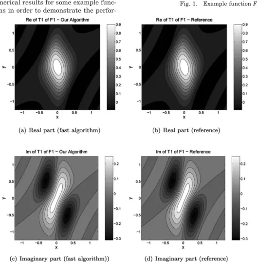
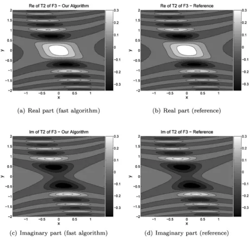
Fast and accurate computation of two-dimensional non-separable quadratic-phase integrals

Ascension à pied jusqu'au cratère (à partir de la gare inférieure du Funiculaire) Excursions quotidiennes organisées par les Agences de Tourisme (pour une

CORELAP is a construction program.. chart In construeting layouts. A building outline is not required for CORELAP. It constructs laiyouts by locating rectc\ngu

Genel olarak hem 1930-1939 yılları arasında Almanya ve Türkiye’deki askerî kültür hakkında derin analizleriyle hem de siyasetin ve kültürün biçimlendirilme- sinde

Nevertheless, for longer capacity acquisition lead times or higher costs of contingent capacity, optimal permanent capacity level in general increases as demand variability

H›z›r, Ahmet Yaflar Ocak’›n ‹slâm-Türk ‹nançlar›nda H›z›r Yahut H›z›r-‹lyas Kültü adl› kita- b›nda söyledi¤i gibi bazen hofl olmayan

Note, the terminal graph is disconnected (separated). At the beginning, we shall save the mass centers of the rigid bodies as additional terminals; therefore, we

Çalışma alanında toprak hidrolik özellikleri; infiltrasyon hızı, sorptivite, doygun hidrolik iletkenlik, tarla kapasitesi, solma noktası ve yarayışlı su içeriği

either chronic hypertension (38) or chronic renal disease was shown to increase SOD and GPx activity, but not the antioxidant effects of CAT, implicating that the protective effect