1
A MODIFIED TAYLOR COLLOCATION METHOD FOR PANTOGRAPH TYPE
FUNCTIONAL DIFFERENTIAL EQUATIONS WITH HYBRID PROPORTIONAL
AND VARIABLE DELAYS
*Elçin GÖKMEN, Department of Mathematics, Muğla Sıtkı Kocman University, TURKEY, [email protected] ( https://orcid.org/0000-0003-1208-1875)
Mehmet SEZER, Department of Mathematics, Celal Bayar University, TURKEY, [email protected] ( https://orcid.org/0000-0002-7744-2574)
Received: 14.10.2019, Accepted: 23.12.2019
*Corresponding author DOI: 10.22531/muglajsci.633017 Research Article
Abstract
In this work, high order pantograph type linear functional differential equations with hybrid proportional and variable delays is approximately solved by the modified Taylor matrix method. With this method these functional type differential equations are converted into the matrix form by the Taylor expansion method. The problems are reduced into a set of algebraic equations including Taylor coefficients. By determining the coefficients, the approximate solutions are calculated. Also, an error analysis technique with residual function is developed for the presented method. Some illustrative examples are given to demonstrate the efficiency and applicability of the method. The computer algebraic system Maple 15 is used for all calculations and graphs.
Keywords: Functional differential equations, Proportional and variable delays, Taylor polynomials and series, Numerical solutions, Residual error analysis.
KARIŞIK ORANLI VE DEĞİŞKEN GECİKMELİ PANTOGRAF TİPİ FONKSİYONEL
DİFERANSİYEL DENKLEMLER İÇİN GELİŞTİRİLMİŞ TAYLOR SIRALAMA
METODU
ÖzetBu çalışmada karışık oranlı ve değişken gecikmeli yüksek mertebe lineer pantograf tip fonksiyonel diferansiyel denklemler geliştirilmiş Taylor matris metotla yaklaşık olarak çözülmüştür. Bu metotla fonksiyonel tip diferansiyel denklemler Taylor açılım metodu ile matris forma dönüştürülür. Problemler Taylor katsayılı cebirsel denklem kümesine indirgenir. Katsayılar belirlenerek yaklaşık çözümler hesaplanır. Ayrıca, metot için kalan fonksiyonlu hata analizi geliştirilmiştir. Metodun verimlilik ve uygulanabilirliğini göstermek için bazı açıklayıcı örnekler verilmiştir. Tüm hesaplamalar ve grafikler için Maple 15 programlama dili kullanılmıştır.
Anahtar Kelimeler: Fonksiyonel diferansiyel denklemler, Nispi ve değişken gecikmeler, Taylor polinomları ve serileri, Nümerik çözümler, Residual hata analizi.
Cite
Gökmen, E., Sezer, M. (2020). “A modified Taylor collocation method for pantograph type functional differential equations with hybrid proportional and variable delays”, Mugla Journal of Science and Technology, 6(1), 1-7.
1. Introduction
In this paper our aim is to obtain a numerical solution of pantograph type functional differential equations with mixed proportional and variable delays in the form
∑ ∑ 𝑃𝑘𝑗(𝑥)𝑦(𝑘)(𝛼𝑘𝑗𝑥 + 𝜏𝑘𝑗(𝑥)) 𝑟 𝑗=0 𝑚 𝑘=0 = 𝑓(𝑥) (1) with the mixed conditions
∑ (𝑎𝑖𝑘𝑦(𝑘) 𝑚−1
𝑘=0
(a) + 𝑏𝑖𝑘𝑦(𝑘)(b)) = 𝜇𝑖 (2)
where 𝑖 = 0,1,2, … , 𝑚 − 1.
Here 𝑃𝑘𝑗(𝑥), 𝜏𝑘𝑗(𝑥) and 𝑓(𝑥) are given and analytical
functions on the interval [𝑎, 𝑏], 𝛼𝑘𝑗, 𝑎𝑘𝑖, 𝑏𝑘𝑖 and 𝜇𝑖 are
given constants with 0 < 𝛼𝑘𝑗< 1, 𝑘 = 0,1, … , 𝑚.
Functional differential equations with proportional and variable delays in the form (1) represent more general class of delay differential equations. They are frequently used to model a wide class of problems in many scientific fields as much as engineering, chemical reactions, mathematical physics, biology, ecology, economics, fluid and elastic mechanics, dynamical systems, population dynamics, signal processing and industrial processes. But most of these equations can not be solved exactly. Therefore, it is necessary to
m
2 design efficient numerical methods to approximate their solutions.
Up to now, Dix [1] analyzed asymptotic behaviour of solutions of first order differential equations with variable delays, Liu et al. [2] established a new sufficient condition for existance, uniqeness of periodic solutions of a Liénard equation with delay, Schley et al.[3] and Zhang[7] studied about determination of linear stability properties for an ordinary differential equation with a varying time delay, Graef and Qian [4], Caraballo and Langa[5] examined attractivity of delay equations, Diblik et al. [6] gave a sufficient conditions for the existence of positive solutions of a scalar linear differential equation with time-dependent delay. Also, numerical methods are studied to solve these type of equations such as the rational approximate method [8], collocation method [9], multistep methods [10], Runge-Kutta methods [11,12] an one-leg-𝜃 methods [13,14]. Here a new numerical technique is developed by modifying matrix methods which have been used by Sezer and coworkers [15-16]. Solutions obtained from this method is expressed in the form
𝑦(𝑥) = ∑ 𝑦𝑛𝑥𝑛 𝑁
𝑁=0
. (3)
Here, 𝑦𝑛, 𝑛 = 0,1, … , 𝑁 are the Taylor coefficients which
are needed to be computed. 2. Fundamental Matrix Relations
In this episode, equation (1) is transformed to a matrix equation. All relations which are needed are given respectively for this transformation. Therefore, let us
first consider the approximate solution 𝑦(𝑥) and its derivatives 𝑦(𝑘)(𝑥), 𝑘 = 1,2, … , 𝑛 defined by truncated
Taylor series. Then we write the matrix form of (3) and its derivatives 𝑦(𝑥) = 𝐗(𝑥)𝐘 (4) 𝑦(𝑘)(𝑥) = 𝐗(𝑥)𝐁𝑘𝐘 (5) where
2 0 1 2 1 X Y ( ) N T N x x x x y y y y 0 1 0 0 0 0 0 2 0 0 0 0 0 3 0 0 0 0 0 0 0 0 0 0 B NBy putting 𝑥 → 𝛼𝑘𝑗𝑥 + 𝜏𝑘𝑗(𝑥) in the relation (5), we
obtain 𝑦(𝑘)(𝛼 𝑘𝑗𝑥 + 𝜏𝑘𝑗(𝑥)) = 𝐗 (𝛼𝑘𝑗𝑥 + 𝜏𝑘𝑗(𝑥)) 𝐁𝑘𝐘 = 𝐗(𝑥)𝐌(𝛼𝑘𝑗, 𝜏𝑘𝑗)𝐁𝑘𝐘 (6) where
0 0 0 1 0 2 0 1 0 1 1 1 1 2 0 1 2 0 1 2 0 0 0 0 1 2 0 1 1 1 2 0 0 2 2 0 0 M ( ) ( ) ( ) ( ) ( ) ( ) ( ) , ( ) ( ) ( ) N kj kj kj kj kj kj kj kj N kj kj kj kj kj kj N kj kj kj kj kj kj N x x x x N x x x x N x x
0 0 N kjN kj( )x N If the relation (6) is substituted into equation (1) we gain the matrix equation as:
∑ ∑ 𝑃𝑘𝑗(𝑥)𝐗(x)𝐌(𝛼𝑘𝑗, 𝜏𝑘𝑗(𝑥𝑟))𝐁𝑘 𝑟 𝑗=0 𝐘 𝑚 𝑘=0 = 𝑓(𝑥𝑟) (7)
2.1. Matrix Representation of Conditions
To find the matrix form of conditions, we substitude the relation (5) in equation (2). Hence, we get the following
equation ∑ [𝑎𝑖𝑘𝐗(𝑎) + 𝑏𝑖𝑘𝐗(𝑏)] 𝑚−1 𝑘=0 𝐁𝑘𝐘 = 𝜇 𝑖 (8) where i= 0,1, … , 𝑚 − 1. 3. Method of Solution
Here by using the matrix equations (7) and (8), we get the approximate solution of (1) under the conditions (2). For this reason by placing the collocation points defined as
𝑥𝑟= a +
𝑏 − 𝑎
𝑁 𝑟, 𝑟 = 0,1, … , 𝑁 (9) into equation (7), we gain the system of matrix equations for 𝑟 = 0,1, … , 𝑁, ∑ ∑ 𝑃𝑘𝑗(𝑥𝑟)𝐗(𝑥𝑟)𝐌(𝛼𝑘𝑗, 𝜏𝑘𝑗(𝑥𝑟))𝐁𝑘 𝑟 𝑗=0 𝐘 𝑚 𝑘=0 = 𝑓(𝑥𝑟) (10)
Thus, the compact form of the system (10) can be written as
3 (∑ ∑ 𝑃𝑘𝑗𝐗̅𝐌̅kj𝐁𝑘 𝑟 𝑗=0 𝑚 𝑘=0 ) 𝐘 = 𝐅 (11) where
0 1 0 1 0 1 P X M , , , ( ) ( ) ( ) ( ) ( ) ( ) ( ( )) ( ( )) ( ( )) kj kj kj kj N N kj kj kj kj kj kj kj kj kj kj N diag P x P x P x diag X x X x X x diag M x M x M x 0 0 1 1 B B B Y F B ( ) ( ) , , . ( ) k k k k N N y f x y f x y f x In Equation (11), the full dimensions of the matrices 𝐏𝑘𝑗, 𝐗,̅ 𝐌̅𝑘𝑗,Bk, 𝐘 and 𝐅 , are respectively (𝑁 + 1) ×
(𝑁 + 1), (𝑁 + 1) × (𝑁 + 1)2, (𝑁 + 1)2× (𝑁 + 1)2, (𝑁 +
1)2× (𝑁 + 1), (𝑁 + 1) × 1 and (𝑁 + 1) × 1.
Also, the fundamental matrix equation (11) can be expressed in the form
𝐖𝐘 = 𝐅 or [ 𝐖; 𝐅] (12) where 𝐖 = [𝑤𝑝𝑞] = ∑ ∑ 𝑃𝑘𝑗𝐗̅𝐌̅kj𝐁𝑘 𝑟 𝑗=0 𝑚 𝑘=0
Similarly, by using relation (8), the matrix form of conditions is written in the form:
𝐕𝒊𝐘 = μ𝒊 or [ 𝐕𝒊; μ𝒊] (13) where 𝑖 = 0,1, . . . , 𝑚 − 1 𝑉𝑖= ∑ [𝑎𝑖𝑘𝐗(𝑎) + 𝑏𝑖𝑘𝐗(𝑏)] 𝑚−1 𝑘=0 𝐁𝑘 = [vi0 vi1 viN].
Consequently, to obtain the solutions of Equation (1) under the conditions (2), we replace the row matrices (13) by any m rows of the matrix (12). So
we get the following new augmented matrix
[𝐖̃ ; 𝐅̃]. (14)
If r𝑎𝑛𝑘(𝐖̃ ; 𝐅̃) = 𝑟𝑎𝑛𝑘(𝐖̃ ) = 𝑁 + 1 , then the unknown coefficients 𝑦0, 𝑦1, … , 𝑦𝑁 are uniquely determined from
the system. Thus, if the determined coefficients are substituted into equation (3), the Taylor polynomial
solution is obtained as the following 𝑦𝑁(𝑥) = ∑ 𝑦𝑛𝑥𝑛.
𝑁
𝑁=0
(15)
Accuracy of the approximate solutions is checked by substituting the solutions into the equation (1)
𝐸𝑁= |∑ ∑ 𝑃𝑘𝑗(𝑥)𝑦𝑁(𝑘)(𝛼𝑘𝑗𝑥 + 𝜏𝑘𝑗(𝑥)) 𝑟 𝑗=0 𝑚 𝑘=0 − 𝑓(𝑥)|. (16) Here if 𝑦𝑁(𝑥) ≅ 𝑦(x), then 𝐸𝑁(𝑥) ≅ 0.
4. Residual Error Analysis
In this section, by using the residual correction method [17-19] we present an error estimation for the Taylor series solution of (1). Our aim is to predict the optimal M which is gived the minimal absolute error. By
modifying the procedure [17-19] to Equation (1), we get the residual function for Taylor polynomial solution (3) as 𝑅 = ∑ ∑ 𝑃𝑘𝑗(𝑥)𝑦𝑁(𝑘)(𝛼𝑘𝑗𝑥 + 𝜏𝑘𝑗(𝑥)) . 𝑟 𝑗=0 𝑚 𝑘=0
If R is added into both sides of Equation (1), we get ∑ ∑ 𝑃𝑘𝑗(𝑥)𝑒𝑁(𝑘)(𝛼𝑘𝑗𝑥 + 𝜏𝑘𝑗(𝑥)) 𝑟 𝑗=0 𝑚 𝑘=0 = −𝑅 (17) where 𝑒𝑁(𝑥) = 𝑦(𝑥) − 𝑦𝑁(𝑥). If ‖𝑒𝑁(𝑥) − 𝑒𝑁,𝑀‖ ≤ 𝜀
is sufficiently small where 𝑒𝑁,𝑀 is Taylor series solution
of (17), then the absolute error can be predicted bye 𝑒𝑁,𝑀. Should 𝑦𝑁(𝑥) be Taylor series solution of (1),
𝑦𝑁,𝑀(𝑥) = 𝑦𝑁(𝑥) + 𝑒𝑁,𝑀(𝑥) named as corrected
approximate solution is also a solution of (1). 5. Illustrative Problems
In this section, some problems are given to understand how the method is progressing and how effective and precise it is.
Problem 1. Let us consider the following functional differential equation with the initial conditions
𝑦′′(𝑥) + 𝑦′(𝑥 − 𝑠𝑖𝑛𝑥) + 2𝑥𝑦(𝑥) = f(x)
𝑦(0) = −1, 𝑦′(0) = 0
where 𝑓(𝑥) = 2 − 2xcosx − 2sinx + 2sinxcosx + 2𝑥3
For the interval [0,1] the set of collocation points for 𝑁 = 2 becomes {𝑥0= 0, 𝑥1=12, 𝑥2= 1}. By using the
4 corresponding augmented matrix [𝐖̃ ; 𝐅̃] the Taylor coefficients are uniquely determined as
𝑌 = [−1 0 1]. Finally, if these determined coefficients are substituted into (3), the approximate solution is obtained as 𝑦(𝑥) = 𝑥2− 1 . That is also the
exact solution of the equation.
Problem 2. For the present example, we examine the equation as
2𝑦′(𝑥) − 𝑥𝑦(𝑥) + 𝑥𝑒2𝑥2𝑦(𝑥 − 𝑥2) = 4𝑒2𝑥
under the initial condition 𝑦(0) = 1 which has the exact solution as 𝑦(𝑥) = 𝑒2𝑥. By using the way in section 3
and taking 𝑁 = 5,7,10,14 we compute the approximate solutions. For 𝑁 = 5 the numerical solution which is obtained as
𝑦5(𝑥) = 1 + 2.0000𝑥 + 1.97936𝑥2+ 1.47227𝑥3
+ 0.323343𝑥4+ 0.610519𝑥5.
All other results are given with tables and figure. Numerical datas of solutions for (𝑁, 𝑀) = (7,10), (10,13) are presented in Table 1. According to this table, it is obvious that as the values of N,M are increased the approximate solutions 𝑦𝑁(𝑥) and 𝑦𝑁,𝑀(𝑥)
are approaches to the exact solution. In Table 2, it is seen that the errors are decrease when N,M values get bigger. Additionaly, the results are shown that 𝑒𝑁,𝑀(𝑥)
calculated by the residual function is closer to zero than 𝑒𝑁(𝑥). Also, in Figure 1 the graphics of corrected
absolute errors are plotted for different (N,M).
Figure 1 shows that if the values N,M increase then the absolute errors decrease.
Figure 1.“Corrected absolute errors”of Problem 2 for varied N,M values.
Problem 3. For the third example we choose the following problem as
𝑦′′′(𝑥) − 𝑦′′(𝑥 − 𝑥2) + 𝑦(𝑥) = 𝑥 − 𝑒𝑥2−𝑥
with the initial conditions
𝑦(0) = 1, 𝑦′(0) = 0, 𝑦′′(0) = 1.
The exact solution of this problem is 𝑦(𝑥) = 𝑥 + 𝑒−𝑥.
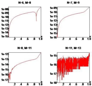
Outputs of this equation are given in Table 3, Table 4 In Figure 2, corrected absolute errors are presented for different N,M.
Figure 2.“Corrected absolute errors”of Problem 3 for varied N,M values.
6. Conclusion
In this paper, we are presented a matrix method based on the Taylor polynomial to solve the pantograph type functional differential equations with hybrid proportional and variable delays. The residual error function is defined for these type of equations to predict the absolute error. Also, it is indicated how the mentioned method and the error analysis prosedures are perfomed on some problems When the problems are examined it is seen that the Taylor polynomial coefficients are found very easily by using computer program written in Maple 15. The numerical results show that if truncation limit N is increased, it can be seen that approximate solutions get closer to the exact solutions. In addition, the technique can also be extended to other type of equations and systems with some modifications.
7. Refrences
[1] Dix, J.G., "Asiymptotic behaviour of solutions to a first-order differential equation with variable delays",
Computers and Mathematics with Applications, 50,
5 [2] Liu, X.G., B., Tang, M.L., Martin, R.R., "Periodic solution for
a kind of Lienard Equation", Journal of Computational and
Applied Mathematics, 219,1, 263-275, 2008.
[3] Schley, D., Shail, R. Gourley, S.A., "Stability criteria for differential equations with variable time delays",
International Journal of Mathematical Education in Science and Technology, 33, 3, 359-375, 2002.
[4] Graef, J.R. and Qian, C. "Global attractivity differential equations with variable delays", J. Austral. Math. Soc. Ser.
B, 41, 568-579, 2000.
[5] Caraballo, T. and Langa, J.A., "Attractors for differential equations with variable delays", J. Math. Anal. Appl., 260, 421-438, 2001.
[6] Diblik, J., Svaboda, Z., Smarda, Z. "Explicit criteria for the existence of positive solutions for a scalar differential equation with variable delay in the critical case",
Computers and Mathematics with Applications., 56,
556-564, 2008.
[7] Zhang, B. "Fixed points and stability in differential equations with variable delays", Nonlinear Analysis, 63, 233-242, 2005.
[8] Ishawata, E. and Muroya, Y. "Rational approximation method for delay differential equations with proportional delay", Applied Mathematics and Comput., 187,2, 741-747, 2007.
[9] Ishawata, E., Muroya, Y., Brunner, H. "A super-attainable order in collocation methods for differential equations with proportional delay" Applied Mathematics and
Comput., 198,1, 227-236, 2008.
[10] Hu, P., Huang, C., Wu, S. "Asymptotic stability of linear multistep methods for nonlinear neutral delay differential equations", Applied Mathematics and Comput., 211,1, 95-101, 2009.
[11] Bellen, A. and Zennaro, M. Numerical methods for delay differential equations in Numerical Mathematics and Scientific Computations, Oxford University Press, New York, 2003.
[12] Wang, W., Zhang, Y., Li, S., "Stability of continuous Runge – Kutta type methods for nonlinear neutral delay-differential equations", Applied Mathematical Modelling, 33,8, 3319-3329, (2009).
[13] Wang, W.S and Li, S., "On the one-leg h-methods for solving nonlinear neutral functional differential equations", Applied Mathematics and Comput, 193,1,285-301, 2007.
[14] Wang, W, Qin, T., Li, S.,"Stability of one-leg h-methods for nonlinear neutral differential equations with proportional delay", Applied Mathematics and Comput, 213,1, 177-183,2009.
[15] Sezer, M. Daşcioglu, A. A., "A Taylor method for numerical solution of generalized pantograph equations with linear functional argument ", Journal of Computational and
Applied Mathematics, 200, 217-225,2007.
[16] Gokmen, E. Sezer, M. " Approximate solution of a model describing biological species living together by Taylor collocation method", New Trends in Math. Sci., 3,2,147-158, 2015.
[17] Oliveira, F. A., "Collocation and residual correction",
Numer Math., 36, 27– 31, 1980.
[18] Çelik, I., "Approximate calculation ofeigenvalues with the method of weighted residual collocation method", Applied
Mathematics and Computation, 160, 2, 401-410, 2005.
[19] Çelik, I., "Collocation method and residual correction using Chebyshev series", Applied Mathematics and
Computation, 174,2, 910-920, 2006.
6
Table 1. Comparisons of solutions of Problem 2 for (𝑁, 𝑀) = (7.10), (10,13).
i x “Exact solution” ( ) 2xi i y x = e “Approximate” “solution”for N=7 y x7( )i “Corrected” “approximate” solution” 7,10( )i y x “Approximate” “solution”for N=10 10( )i y x “Corrected” “approximate” “solution” y10,13( )xi Numerical values 0 1 1.00000000000 1.00000000000 1.00000000000 1 0.2 1.49182469764 1.49182370972 1.49182469793 1.49182469792 1.49182469766 0.4 2.22554092849 2.22553996766 2.22554092879 2.22554092876 2.22554092851 0.6 3.32011692274 3.32011612513 3.32011692309 3.32011692299 3.32011692276 0.8 4.95303242440 4.95303209614 4.95303242475 4.95303242459 4.95303242437 1.0 7.38905609893 7.38902007967 7.38905608402 7.38905608372 7.38905609884
Table 2. Comparisons of the absolute errors of Problem 2 for ( ,N M =) (10,13), (14,16).
i
x
“Actual absolute errors”for N=10
e10( )xi
“Estimated absolute errors”for N=10 and M=13 e10,13( )xi
“Corrected absolute errors” for N=10 and M=13 E10,13( )xi
0 0 0 0
0.2 0.2712e-009 0.2697e-009 0.3249e-011
0.4 0.2795e-009 0.2763e-009 0.7633e-011
0.6 0.2636e-009 0.2645e-009 0.1215e-011
0.8 0.1865e-009 0.1887e-009 0.2545e-010
1.0 0.1521e-007 0.1521e-007 0.8974e-010
i
x
“Actual absolute errors” for N=14
e14( )xi
“Estimated absolute errors” for N=14 and M=16 e14,16( )xi
“Corrected absolute errors” for N=14 and M=16 E14,16( )xi
0 0 0 0
0.2 0.1112e-011 0.1957e-014 0.3512e-017
0.4 0.2059e-011 0.1934e-014 0.3475e-017
0.6 0.3849e-011 0.1864e-014 0.3352e-017
0.8 0.5783e-011 0.1640e-014 0.2942e-017
1.0 0.7561e-012 0.1461e-012 0.3007e-015
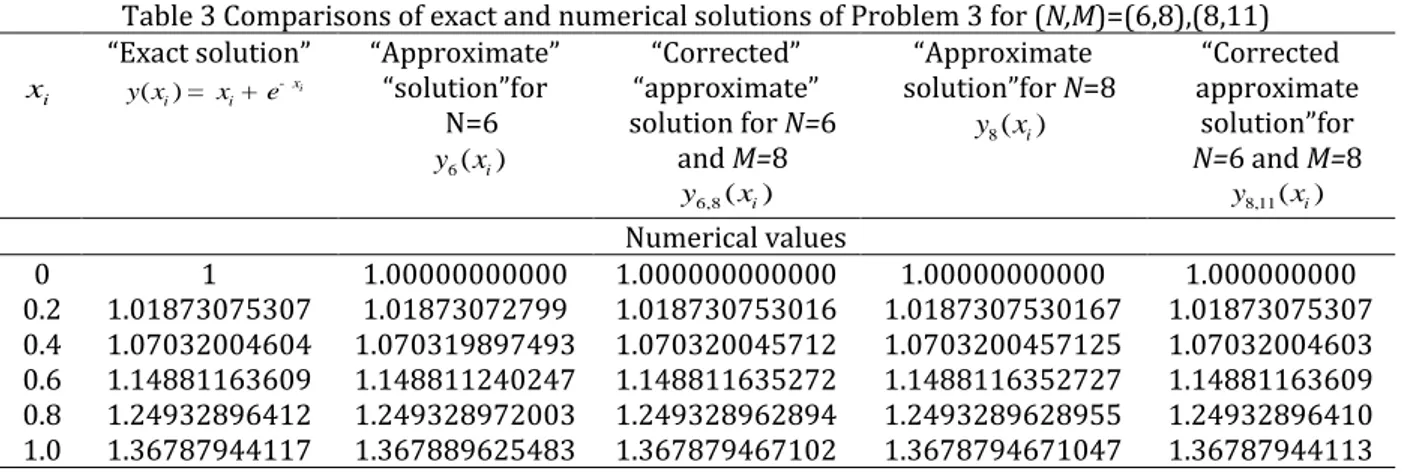
Table 3 Comparisons of exact and numerical solutions of Problem 3 for (N,M)=(6,8),(8,11)
i x “Exact solution” ( ) xi i i y x = x+e -“Approximate” “solution”for N=6 6( )i y x “Corrected” “approximate” solution for N=6 and M=8 6,8( i) y x “Approximate solution”for N=8 y x8( )i “Corrected approximate solution”for N=6 and M=8 y8,11(xi) Numerical values 0 1 1.00000000000 1.000000000000 1.00000000000 1.000000000 0.2 1.01873075307 1.01873072799 1.018730753016 1.0187307530167 1.01873075307 0.4 1.07032004604 1.070319897493 1.070320045712 1.0703200457125 1.07032004603 0.6 1.14881163609 1.148811240247 1.148811635272 1.1488116352727 1.14881163609 0.8 1.24932896412 1.249328972003 1.249328962894 1.2493289628955 1.24932896410 1.0 1.36787944117 1.367889625483 1.367879467102 1.3678794671047 1.36787944113
7
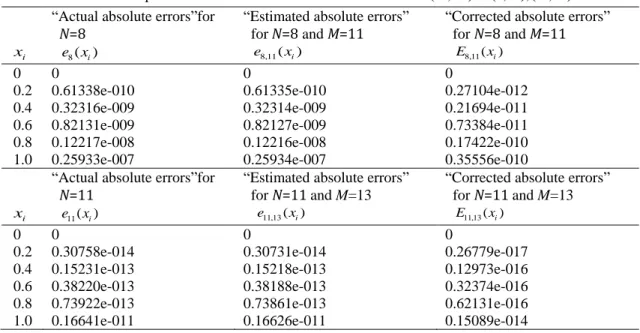
Table 4. Comparison of the absolute errors of Problem 3 for ( ,N M =) (8,11), (11,13).
i
x
“Actual absolute errors”for N=8
e x8( )i
“Estimated absolute errors” for N=8 and M=11 e8,11(xi)
“Corrected absolute errors” for N=8 and M=11 E8,11( )xi
0 0 0 0
0.2 0.61338e-010 0.61335e-010 0.27104e-012
0.4 0.32316e-009 0.32314e-009 0.21694e-011
0.6 0.82131e-009 0.82127e-009 0.73384e-011
0.8 0.12217e-008 0.12216e-008 0.17422e-010
1.0 0.25933e-007 0.25934e-007 0.35556e-010
i
x
“Actual absolute errors”for N=11
e11( )xi
“Estimated absolute errors” for N=11 and M=13 e11,13( )xi
“Corrected absolute errors” for N=11 and M=13 E11,13( )xi
0 0 0 0
0.2 0.30758e-014 0.30731e-014 0.26779e-017
0.4 0.15231e-013 0.15218e-013 0.12973e-016
0.6 0.38220e-013 0.38188e-013 0.32374e-016
0.8 0.73922e-013 0.73861e-013 0.62131e-016