Exact Solutions of the Cauchy Problem for 2-D Scalar Conservation Laws

>

Volume 5(1-2), 2012, 27-47

EXACT SOLUTION OF THE CAUCHY PROBLEM FOR 2-D SCALAR CONSERVATION LAWS WITH CONSTANT COEFFICIENTS IN A CLASS OF DISCONTINUOUS FUNCTIONS

Mahir RESULOV* and Kenan SENTURK**

* BeykentUniversity, Department ofMathematics and Computing, Ayazaga-Maslak Campus, 34396, Istanbul, Turkey

mresulov@beykent.edu.tr

** Beykent University, Department ofEnergy Systems Engineering Ayazaga-Maslak Campus, 34396, Istanbul, Turkey

kenansenturk@beykent.edu.tr ABSTRACT

In this study a new method for finding exact solution of the Cauchy problem subject to a discontinuous initial profile for the two dimensional scalar conservation laws is suggested. For this aim, first, some properties of the weak solution of the linearized equation are investigated. Taking these properties into consideration an auxiliary problem having some advantages over the main problem is introduced. The proposed auxiliary problems also permit us to develop effective different numerical algorithms for finding the solutions. Some computer experiments are carried out.

Keywords: Scalar conservation laws, auxiliary problem, exact and numerical solution in a class of discontinuous functions

ÖZET

Bu çalışmada iki boyutlu skaler korunum kuralları için yazılmış süreksiz başlangıç koşullu Cauchy probleminin gerçek çözümünün bulunması için yeni bir yöntem önerilmiştir. Bu amaçla önce, lineerleştirilmiş denklemin zayıf çözümünün bazı özellikleri incelenmiş ve bu özellikler dikkate alınarak esas problemde bulunmayan ve bazı avantajlara sahip yardımcı problem dahil edilmiştir. Önerilen yardımcı problem göz önüne alınan problemin sayısal çözümünü bulmak için etkin sayısal algoritmalar yazmaya da geniş imkan sağlamaktadır.

Anahtar Kelimeler: Skaler korunum yasaları, yardımcı problem, süreksiz fonksiyonlar sınıfında gerçek ve sayısal çözümler

1. INTRODUCTION

It is known that investigation of many problems in sciences and engineering, particularly in fluid dynamics, requires to study the nonlinear hyperbolic equations of conservation laws. It is typical in such problems that their solutions admit the points of discontinuity whose locations are unknown beforehand. Therefore, even in one dimensional case they pose a special challenge for theoretical and numerical analysis.

The mathematical theory of the Cauchy problem for one dimensional nonlinear hyperbolic equation is studied in [4], [8], [9], [13], [21], [25]. Profound results for the mathematical theory of the initial boundary value problem for scalar conservation laws in several space dimensions can be found in [1], [3], [6], [7]. Most hyperbolic equations (or systems) of conservation laws in physics are nonlinear and solving them analytically is often difficult, sometimes impossible.

There are many sensitive numerical methods for the solving of the Cauchy problem of nonlinear hyperbolic equations [2], [8], [10], [12] and etc. Very relevant results to the basis of the main themes are found [5], [6], [11], [22], [23], [24].

In this study the original method for finding the exact and numerical solution of the Cauchy problem for the two dimensional scalar equation

X y ,t ) | dF1(u(x,y,t)) | dF2{u{x,y,t)) = Q

dt dx dy

is suggested. The conditions which the functions Fi (u),(i = 1,2)

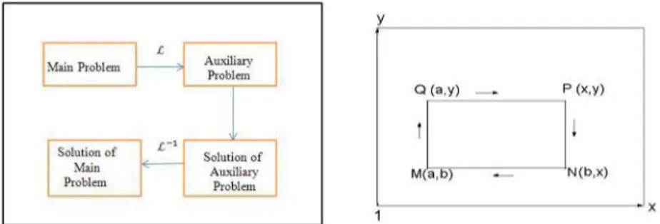
must satisfy will be expressed in section 3, later. For this aim, the special auxiliary problem having some advantages over the main problem is introduced. The suggested auxiliary problem permits us in some cases to construct the exact solution of the investigated problem in a class of discontinuous functions, and to develop sensitive algorithms for obtaining the numerical solution of the main problem. The principle application of the proposed method is schematically shown in Figure 1a.

Q ( a , y ) — P (x,y)

t I

M(a,b) - — N(b,x)

Figure 1: a) Schematic representation of the suggested method; b) Domain D _xy

The Cauchy problem for equation (1), when F ( u ) = F ( u ) = F(u) has been studied in [17], [18] analytically as well as numerically. In order to study in full detail at first the case F ( u ) = Au and F (u) = Bu is considered. Here A and B are given real constants.

2. THE LINEAR EQUATION AND SOME PROPERTIES OF THE EXACT SOLUTION

Let R = R2 x[0, T) be Euclidean space of the points (x, y, t),

where ( x , y ) e R2, t e[0,T) and T is a given constant. In R3+ we

consider the following Cauchy problem

du( x, y, t )+A du( x, y, t) | ^ du( x, y, t) = Q

dt dx u( x, y,0) = uo( x, y).

dy (2)

(3) Here, u (x, y) is any given measurable and bounded continuous function having both positive and negative slopes. The problem (2), (3) later on will be called as the main problem. We support that

A ^ B and let D„, be the domain defined as follows Dy = { ( ^ ) , a < £ < x, b <V< y} c R2, t e RT+ . By dDy we

denote the boundary of the domain D ., figure 1b It is easily shown that the function

is the exact solution of the main problem, and such solution is called a soft solution of the problem (2), (3).

Definition 1. The function u(x, y, t ) satisfying the initial condition (3) is called a weak solution of the problem (2), (3) if the following integral relation

| | { u(x, y, t)[< (x, y, t) + A<px (x, y, t) + B<y (x, y, t)] }dxdydt

+ J[(x, y,0)u (x, y)dxdy = 0 (5) r2 RT

holds for every test functions ( ( x , y, t) defined in R+ and

differentiable in the upper half plane and vanishes for yjx2 + y2 +1

sufficiently large.

Theorem 1. If the u(x, y, t) is a continuous weak solution of the main problem, then the function u(x, y, t) = u0 (x - At, y - Bt) is a

soft solution of the main problem.

The proofs of the Theorem 1 and Theorem 2 are developed similarly as in [12].

Proof According to the definition of a weak solution we have | J{u(x, y, t)[v (x, y, t) + Avx (x, y, t) + Bvy (x, y, t)] }dxdydt R2 RT

+ J[(x, y,0) u0 (x, y) dxdy = 0 (6)

for every smooth function v(x, y,t) which vanishes for •Jx2 + y2 +1 sufficiently large.

Applying the following transformation of variables

£ = x - At, rj = y - Bt, r = t, (7) (6) can be expressed as 2 R 2 R

J J { u ( £ , r , r ) vT( £ , j , r ) } d £ d r + J v ( £ , r , 0 ) U 0 ( £ , r ) d £ d j = 0

R2 r T

or

J J J u(£, r, r)vr (£, r, r) dj+v(£, r ,0)u(£, r,0) I d£ = 0

r 2 t 0 J

for every smooth v( x, y, t ) with appropriate support. If we define F (£,r)

= J

u ( £ ,

r

, r ) v

r

( £ ,r, r ) d r

0

then the previous relation can be rewritten as

J F (£,r)+u(£,r,0)v(£,r,0)] = 0.

R2

This implies that F(£,r) + u(£,j,0)v(£,j,0) = 0 for, if there were and domain ,£2 , ] x [ j ] where this is different from zero.

Then we have

J [ F (£,r)+u(£,r,0)v (£,r,0)]d£dj > 0,

R2

which is a contradiction. We conclude that

J u(£, j , r)vr (£, r , r) dr + v(£, r,0)u(£, j ,0) = 0.

Since, J vT( £ , r , r ) d r = - v ( £ , j , 0 ) , then

and we get

J vr (£, j , r)u(£, j ,0) d r = -v(£, j ,0)u (£, j,0),

J[ u ( £ J, r ) - u (^ j ) ] vr(£ j, r ) d r = 0.

From the continuity of u we conclude that

u(£,j,r) = u ( £ , j ) = u (x - At, y - Bt). 2 R T R ₊ T R ₊ T R ₊ T R ₊

Theorem 2. If u0 (x - At, y - Bt) is integrable, then the function

u(x, y, t) defined by the formula (4) is a weak solution of the main

problem.

Proof Let v be a smooth function which vanishes for yjx2 + y2 +1

sufficiently large. Consider the expression

J Ju0 (x - At, y - Bt){ vt (x, y, t) + Avx (x, y, t) + Bvy (x, y, t) ]dxdydt R2 RT+

+ J v(x, y,0)u0 (x, y) dxdy.] (8)

R2

Taking account into consideration the (7), we have

J J u0( l ; , r ¡ ) vT( % , r , r ) d % d r ¡ d T + J v ( x , y , 0 ) u0( x , y ) d x d y .

R2 rT

During the integration with respect to T , since v = 0 for sufficiently large T , the sum of these integrals vanishes. Hence, the function u(x, y, y) = u0 (x - At, y - Bt) is a weak solution of the

main problem.

Integrating the equation (2) on the domain with respect to x, y and using the Green's formula we get

s x y — U t) + | Audy - Budx = 0 St' h a n a b xy or a x y q j j 7 , t ) d^d7 + Aj[u(x, 7, t) - u(a, 7, t)] d7 a b x - B

J\u

a

The last equation can be rewritten as

x y y B

j

[w(£ y, t) - u(g, b, t )]dğ = 0. S j j t ) d%dv + Aju(x,7, t) dv St , _{a b} R2 b

-

BJ

u(£, y, t )dg = p(a, y, t) X, b, t).

a

(9)

y x

Here, p(a, y, t) = u(a, 77, t)d77, X, b, t) = BJu(£, b, t)d£.

The problem finding the solution of the equation (9) subject to (3) will be called as first auxiliary problem.

We introduce the following operator 3(0 = ^

dxdy

(10)

and the function defined as

x y

v(X, y, t) = J Ju(£, 77, t)d&v + Q (a, y, t) - % (X, b, t), (11) where %(X, b, t) and ^ ( a , y, t) are the integrals of y/(X, b, t) and

p(a, y, t) with respect to t, respectively. It is easily shown, that the

function p(a, y, t) X, b, t) e ker3. Indeed,

3 [ p ( a , y, t) - IY( X, b, t)] = 3 AJ u(a,7, t )d7 + BJ u(%, b, t )d% = 0.

For the sake of simplicity, we denote H (a, b, X, y, t) = p(a, y, t) - \Y( X, b, t) and it is obvious that 3 H (a, b, X, y, t) = 0.

Taking into consideration (11), the equation (9) takes the form

dv ( X y, t )+A S v ( x1y ,t ) + B d v ( X y, t ) = Q

(12)

dt dx dy

The initial condition for the equation (12) is

v( X, y,0) = Vo(x, y), (13)

here the function v0(x, y) is any solution of the equation

b a

X

From (11) we have

= X. y). (14)

oxdy

d 2v( x. y. t)_

dxdy = u(x. y. t). (15)

Indeed, if we differentiate the relation (12) at first with respect to x , then with respect to y we prove validity of (15).

The problem (12), (13) will be called second auxiliary problem. The second auxiliary problem has the following advantages:

• The differentiability property of the function v(x, y, t) with respect to X and y is two orders higher than u(x, y, t)

• The function u(x, y, t) may be discontinuous.

• By obtaining the solution u(x, y, t) of the problem (12), (13), we does not use the derivatives uX, u , ut, which does not

already exist, usually.

It is obvious that the solution of the auxiliary problem is not unique. The following theorem is valid:

Theorem 3. If the function v(x, y, t) is soft solution of the auxiliary problem (12), (13), then the function u(x, y, t) defined by (15) is a weak solution of the main problem.

Proof Let the function p(x, y, t) is a test function and we consider the following expression

r I d v d v d v I

0 = | 3 p ( x , y, t)<— + A— + B— \dxdydt. ¿3 [ S t d x d y J

After some simple manipulation we get

r , J d 3 v , d 3 v nd 3 v | . . .

I p(x, y, t K + A + B \dxdydt = 0.

Applying integration by part to the last equality with respect to t,

x, y respectively have

JV(

x y>t )i

Su(x,y,t) .Su(x,y,t) i BSu(x,y,t)

• + A 1

St dx + B- Sy \dxdydt = 0.

This completes the proof.

3. TWO DIMENSIONAL SCALAR CONSERVATION LAW In this section the two dimensional scalar equation which describes a certain conservation law as

du^ SF1 (u) | SF2 (u) = o

St Sx Sy (16)

is considered. We assume that the equation is subjected to the initial condition (3).

Relatively F (u) and F (u) we assume that

(i) F (u) and F (u) are continuous differentiable functions, (ii) F ( u ) > 0, (i = 1,2) for u > 0,

(iii) F'(u) has an alternative signs, t.e. the Fi (u), (i = 1,2)

functions have the concave and convex parts.

The solution of the problem (16), (3) obtained using the characteristics method is

u (

x ^

t )

=

u

o

(

^

,r

^)

, (17) where £ = x - F'(u)t and TJ = y - F2'(u)t are the special coordinates

moving with speed of F((u) and F[(u), respectively. From (17) we get Sun Su Sx ( 1 + Fi ' ( u ) ^ + F2 (u) Su S uo S77 t 3 R ₊

du dy du ~dt du0 d^ 1 + f » ^ + F » ^du du 0 dç d^ F(u) d u0 + F » du0 dç d77 f 1 + Fan) du0+Fî(u) du 0 dç d77

As it is seen from this formulas, if —0 < 0 , —0 < 0 and

d'q

F '(u) > 0, (i = 1,2) (or d U o> 0 , d U o > 0 and F (u) < 0) at the

dÇ

d^

value

t > T0 =

1 F_"(u) duo + F2"(u)

the derivatives ux, u and ut are approaching to infinity. Therefore

the classical solution of the problem (16), (3) does not exist. The weak solution of the problem (16), (3), we will be defined as follows.

Definition 2. The function u(x, y, t) satisfying the initial condition (3) is called a weak solution of the problem (16), (3) if the following integral relation

J J J { u(t + F (u)(x + F2 (u)( ]dxdydt R2 RT+

+ J J u0 (x, y ) ( ( x, y,0) dxdy = 0 (18)

holds for every test functions ( ( x , y, t) defined in R+ and

differentiable in the upper half plane and vanishes for -J. sufficiently large. .x2 + y2 +1 t t 2 R

In order to find the weak solution of the problem (16),(3) in sense (18) we will introduce the auxiliary problem as above. Integrating the equation (16) on the region D we get

0 =

if<

xy Su SF (u) SF2 (u) St S] \d£d]

f J J u ( £ ]

t

) ^

d

r + J J

SF1(u) SF• + 2(u) S St D xy x y S£ Sr] , d£d] x y y

J J u(£,], t )d£d r] + J\_F (u( x, ] , t))- F (u(a, ] , t ))]d]

b a b

+ J F 2 (u(£, y, t ) ) - F2 (u(£, b, t ))]d£.

The last equality can be rewritten as

Q x y y x

— J Ju(£, r, t)d£dr + J Fi (u(x, r, t))dr + J F2 (u(£, y, t))d£

b a = 0(a, y, t ) + T ( x , b, t). ab Here y x 0 ( a , y, t) = J F (u(a,r, t))d], x, b, t) = JF2 (u(£, b, t))d£. It b a

is clearly seen that 0 ( a , y, t) + ¥ ( x , b, t) e ker 3 . Indeed,

3 { 0 ( a , y, t) + x, b, t)} = 3 J F (u(a, ], t ))d] + J F2 (u(£, b, t ))d£

_ SF (u(a, y, t)) S F (u(x, b, t)) _ • + - = 0. Sx Sy We denote by v( x, y, t) following expression

D xy

x

a

x

X y

v( y, t) = J J u(Ç, r , t )dÇdr + H (a, b, X, y, t), (19)

a b

where Hx (a, b, x, y, t) e ker 3 . From (19) we have

, d 2v( x, y, t)

u(x,y,t) = v ' .

dxdy

Taking into consideration to (19) we get dv( x, y, t) dt +

M

d 2v( x,r, t) dxd] X

dr+J F

2 d 2v(Ç, y, t) dÇdy dÇ = 0 or dv( x, y, t) dt + J F ( u ( x , r , t ) ) d r + J F ( u ( Ç , y , t ) d = 0. (20)

The initial condition for the (20) is

v ( x, y, 0 ) = v0( x, y). (21)

Here the function v0(x, y) is any differentiable solution of the

equation (14).

The auxiliary problem (20), (3) has following advantages: (i) In this case the functions u(x, y, t), F(u(x, y, t)) and

F (u(x, y, t)) can be discontinuous too,

(ii) the order of differentiability of the function v(x, y, t) more than the order of differentiability of the function u(x, y, t) ,

(iii) the derivatives ux , u and ut in algorithm for obtaining

of the solution of the problem (16) and (3) does not occur, as these derivatives does not exist.

The following theorem is valid.

Theorem 4. If the function v(x, y, t) is solution of the auxiliary problem (20), (3), then the function u(x, y, t) expressed by

u(x, y, t) = 3v(x, y, t) is a weak solution of the main problem (16)

and (3).

b a

X

4. FINITE DIFFERENCES SCHEMES IN A CLASS OF DISCONTINUOUS FUNCTIONS

In this section, we intended to develop the numerical method for finding the solution of the problem (2), (3), and investigate some properties of it. For this aim, we will use the auxiliary problem (9), (3). As it is stated above, in the nonlinear case the solution of the main problem has discontinuous points, whose locations are unknown beforehand. The properties found in the exact solution does not permit us the application of classical numerical methods to this problem directly. In this case we will use the problem (20), (3). By using the advantages of the suggested auxiliary problem, a new numerical algorithm will be proposed. In order to demonstrate the effectiveness of the proposed method in this study we will consider only linear case. In [14], [15], [16] the suggested numerical method was studied for an one dimensional nonlinear scalar equation.

The offered method will be developed to find the numerical solution of the Cauchy problem for the equation (1) in following study.

4.1 The Finite Differences Scheme for Cauchy Problem

By investigating a numerical solution of the Cauchy problem for the equation (1) we will use the ideas and notations presupposed in familiar books [19] and [20].

In order to construct the numerical algorithm, the domain of definition of the problem (2), (3) is covered by the following grid

®h,h2 = { ( x,, yj, tk X xi = K yj = JK tk = k r ,

i = 0,1,2,...; J = 0,1,2,...; k = 0,1,2,...; h >0, h > 0 , r >0},

where, h , h2 and r are steps of the grid with respect to x, y and

t , respectively.

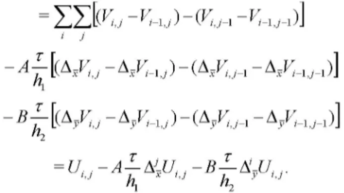
In order to approximate of the equation (9) by the finite differences, the integrals leaving in (9) are approximated as follows

x

a

Y J J u ( t ) d V = h2 /UhM,k , M=1 and X Y ı J J J u(Ç,v, t )dÇd1 = \h2 / / U 2 / J / ^ v , j U , k ' v = 1 ^ = 1 (23) (24) Taking into consideration (22)-(24) the equation (9) at any point

(i, j,k) of the grid ^,r is approximated as follows

j-1 i-1

U, _{i,J k+1} (1 - f A + f BU J,k - f A//U,Mkk + f B/U

h h _M=1 h2 v , j ,k i-1 J - 1 . J-1 S S ( U v ^ k + 1 - Uv,M ) + f A / U o ,Ak - f B / U V , n, k , ( 2 5 ) h 1 ^=1 h v=1 ^ = 1 «2 v=1 (i = 0,1,2, ....N; j = 0,1,2,...,M, k = 0,1, 2,...,). The initial condition for (25) is

U,„0 = ^(-X,y-), (i = 0,1,2,....N; j = 0,1,2,...,M). (26) Now, we approximate the problem (12), (13) by the finite differences. For this aim, we introduce the following notations

U(xt, yj, tk ) = Ui,j, U(x, y,, tk+1) = Ûhj,

A U j = (U„ -Ui-1., X Ay Uu = (U u " j

= (

A

U , -

t f y U u = ^

-

^

j ).

In this notations the problem (12), (13) is approximated by the finite differences scheme as follows

T T

V = v - A— A-V - B— A-V ,

ı , j i,j h x l , J h y l , J V = V(0)

Vi , J , 0 Vi , J •

(27) (28) Here, the function Vi (°) is any continuous solution of the equation

V S = u0(xt, yj), (29)

b

b a

and the grid functions U . and VUj represent approximate values

of the functions u(x, y, t) and v(x, y, t) at point (i, j, k) respectively.

Note 1. It should be noted that A - U = A - U . In order to prove this property, we consider

A xyU - Ax U , j " A xU j i = ( U , j - U - i j h P u - i )

= U, j U - l)-( Ui - , j -Ui - , j i) = AyxU.

It is easy to prove that, if the grid function V,j is the solution the

problem (27), (28), then the grid function U;,j defined by

1

U i j h h

is the solution of the problem

•A-V • _{xy i,j} (30)

T T

U',j = Ui , j - ^ t A U - 5 — KyUiJ , ( 3 1 )

U j 0 = Uo(x, y ) . (32) In order to prove this claim, let us consider the relation

Uu =

ZZ

A

XyVj

=

ZZl^j

- V

-w

)

-

fcj-1 -

W i

)

J

I J

= z z

i j f I J T T V - A—A-V - ^ A - V . i , J h x i , J h y i J V T T 2 y Y y' i - 1 ,j y f T T V . , - A TA - V . , - B - ^ A - V , V i , j - 1 h x i , j - 1 h y i , J - 1 y T T V_{V i-1,j-1} - _{A h A} A — A - V _{xVi - 1 , J - 1} - B — A - V _{B , A yV i - 1 , J - 1} v h2 y

• H S V u - V - U ) - V J - 1 - V - i j - 1 ) ] ' J A^[(AV,, - A VU) - ( A V , j - ! - A V - i j - i ) ] B - [(A- V , - A ^ - u ) - (AV , ; - i - V W i ) ] T T = - A - m j - B - K - U i j .

It is proved the correctness of our claim. 5. NUMERICAL EXPERIMENTS

In this section, in order to demonstrate the suggested method we will carry out some numerical experiments using the suggested method. At first, we will find the exact solution of the auxiliary problem (12), (13), and using the formula (15) the exact solution of the main problem. Next, we will compare these with the solution of the main problem obtained by classical methods.

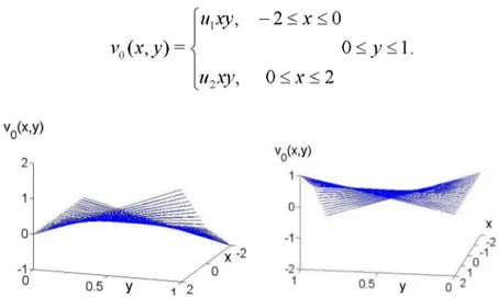
Figure 2: The graph of the function u0 (x, - ) ; a) u > U ; b) U < U

For the sake of simplicity the initial function of the main problem u0 (x, - ) we will take the following form

U, - 2 < x < 0

uo( x y) = < ,0 < y < 1 (33)

where U a nd U are given real constants. In this case, the function vo (x, y) according to (14) is defined as vo( x y) = < Uxy, - 2 < x < 0 0 < y < 1. u2xy, 0 < x < 2

Figure 3: The graph of the function v0 (x, y ) ; a) u > U ; b) U < U

The graphs of the initial functions u0 (x, y) and v (x, y) are shown

in Figure 2 and Figure 3, respectively.

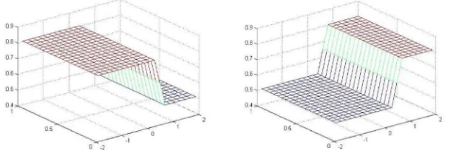
The exact solution of the problem (12), (13) obtained by the characteristics method is

U (x - At)(y - Bt), - 2 < x < 0

v( x, y, t ) = < 0 < y < 1. U (x - At)(y - Bt), 0 < x < 2

Figure 4: The graphs of the function v ( x , y , t ) , A = 0.5, B = 1.0, T = 1.0; a) U > U2 , b) U < U

The graphs of v(x, y, t) at time T = 1.0 are given in Figure 4. The solution of the problem (2), (3) obtained by the formula (15) is demonstrated in Figure 5. On an equal footing the graphs of the exact solution obtained by the formula (4) is given in Figure 6, at value T = 0.6.

Figure 5: The graphs of the function u(x, t, t) = 3 v ( x , y, t) , A = 0.5, B = 1.0, T = 1.0 ; a) U > U , b) U < U

Figure 6: The time evaluation of u(x, y, t) at the value T = 0.6 a) U > U ; b) u < U

6. CONCLUSION

In this study an original method for finding the exact and numerical solutions of the Cauchy problem for the first order 2-D nonlinear partial equations in a class of discontinuous functions is proposed. The properties of the exact solution of the linearized equation are also studied.

The special auxiliary problem whose solution is more smoother than the solution of the main problem is introduced, which makes possible to develop efficient and sensitive algorithms that describe all physical properties of the investigated problem accurately.

REFERENCES

[1] Godlewski, E., Raviart, R.E., Hyperbolic Systems of Conservation Laws, Mathematiques & Applications, 1991.

[2] Godunov, S.K., A Difference Scheme for Numerical Computation of Discontinuous Solutions of Equations of Fluid Dynamics, Mat. Sb. Vol. 47 (89), pp. 271-306, 1959.

[3] Godunov, S.K., Equations of Mathematical Physics. Nauka, Moscow, 1979.

[4] Goritski, A.Y., Krujkov, S.N., Chechkin G.A., First Order Quasi Linear Equations with Partial Derivatives, Pub. of Moscow University, Moscow, 1997.

[5] Guinot, V., Godunov-Type Schemes; An Introduction for Engineers, Elsevier, 2003.

[6] Kroner, D., Numerical Schemes for Conservation Laws, J.Wiley & Sons Ltd and B.G. Tenber, 1997.

[7] Kruzkov, S.N., First Order Quasilinear Equation in Several Independent Variables, Math. Sbornik, 81, pp. 217-243, 1970.

[8] Lax, P.D., Weak Solutions of Nonlinear Hyperbolic Equations and Their Numerical Computations, Comm. of Pure and App. Math, Vol VII, pp. 159-193, 1954.

[9] Lax, P.D., Hyperbolic Systems of Conservation Laws and the Mathematical Theory of Shock Waves. Conf. Board Math. Sci. Regional Conf. Series in Appl. Math. 11, SIAM, Philadelphia,

1972.

[10] Lax, P.D., and Wendrof, B., Systems of Conservation Laws, Los Alamos Scientific Laboratory, LA-2285, 1959.

[11] LeVeque R.J. Finite Volume Methods for Hyperbolic Problems. Cambridge University Press, 2002, 558p.

[12] Noh, W.F., Protter, M.N., Difference Methods and the Equations of Hydrodynamics, Journal of Math. and Mechanics, Vol. 12, No. 2, 1963.

[13] Oleinik, O.A., Discontinuous Solutions of Nonlinear Differential Equations, Usp. Math. Nauk, 12, 1957.

[14] Rasulov, M.A., On a Method of Solving the Cauchy Problem for a First Order Nonlinear Equation of Hyperbolic Type with a

Smooth Initial Condition, Soviet Math. Dok. 43, No.1, 1991. [15] Rasulov, M.A. Finite Difference Scheme for Solving of Some Nonlinear Problems of Mathematical Physics in a Class of Discontinuous Functions, Baku, 1996.

[16] Rasulov, M.A., Ragimova, T.A. A Numerical Method of the Solution of the Nonlinear Equation of a Hyperbolic Type of the First Order Differential Equations, Minsk, Vol. 28, No.7, pp. 2056-2063, 1992.

[17] Rasulov, M.A. Identification of the Saturation Jump in the Process of Oil Displacement by Water in a 2D Domain, Dokl RAN, Vol. 319, No.4, pp. 943-947, 1991.

[18] Rasulov, M.A., Coskun, E., Sinsoysal, B., Finite Differences Method for a Two-Dimensional Nonlinear Hyperbolic Equations in a Class of Discontinuous Functions, App. Mathematics and Computation, vol.140, No.l, pp.279-295, 2003.

[19] Richmyer, R.D., Morton, K.W. Difference Methods for Initial Value Problems, Wiley, Int., New York, 1967.

[20] Samarskii, A.A., Theory of Difference Schemes, Nauka, Moscow, 1977.

[21] Smoller, J.A., Shock Wave and Reaction Diffusion Equations, Springer-Verlag, New York Inc., 1983.

[22] Thomas, J.W., Numerical Partial Differential Equations, Finite Difference methods, Springer-Verlag, 436p, 1995.

[23] Thomas, J.W., Numerical Partial Differential Equations, Conservation Laws and Elliptic Equations, Springer-Verlag, 573p, 1999.

[24] Toro, E.F., Riemann Solvers and Numerical Methods for Fluid Dynamics. Springer-Verlag, Berlin Heidelberg, 1999.

[25] Whitham, G.B., Linear and Nonlinear Waves, Wiley Int., New York, 1974.