Contents lists available atScienceDirect
Journal of Computational and Applied
Mathematics
journal homepage:www.elsevier.com/locate/cam
A numerical approach for solving Volterra type functional
integral equations with variable bounds and mixed delays
Elcin Gokmen
a,∗, Gamze Yuksel
a, Mehmet Sezer
baDepartment of Mathematics, Faculty of Science, Mugla Sıtkı Koçman University, Mugla, Turkey bDepartment of Mathematics, Faculty of Science and Art, Celal Bayar University, Manisa, Turkey
a r t i c l e i n f o Article history:
Received 28 March 2016 Keywords:
Integro functional equations Taylor polynomials Approximate solutions Collocation method
a b s t r a c t
In this paper, the Taylor collocation method has been used the integro functional equation with variable bounds. This method is essentially based on the truncated Taylor series and its matrix representations with collocation points. We have introduced the method to solve the functional integral equations with variable bounds. We have also improved error analysis for this method by using the residual function to estimate the absolute errors. To illustrate the pertinent features of the method numeric examples are presented and results are compared with the other methods. All numerical computations have been performed on the computer algebraic system Maple 15.
© 2016 Elsevier B.V. All rights reserved.
1. Introduction
Integral equations play very significant role linear and nonlinear functional analysis and their applications [1]. They are mostly in connection with functional equations. Functional equations occur with difference, differential and integral forms [2]. (FDE) have been studied in several papers [2–12]. Functional integral equations (FDEs) and their systems have a major importance in modeling many phenomena such as biology, ecology, physics and engineering so they have been studied in several papers [13–18]. An integro functional equation is illustrated by
F
x, ϕ (
x) , ϕ
[f(
x)
],
x x0 Kr(
x,
t, ϕ (
t) , ϕ
[f(
t)
])
dt
=
0.
FDEs are usually difficult to solve analytically; so there are particular methods that have solved them numerically. Up to now to obtain numerical solutions of the first and second kind of functional integral and integro-differential equations have been used an expansion method based on Chebyshev interpolation [7,8], Lagrange collocation method [16], Chebyshev collocation method [9,10], variational iteration method (VIM) [6] and Legendre collocation method [11].
In this article we want to find truncated Taylor series solution of integro functional equation with variable bounds represented by m1
k=0 Pk(
x)
y(α
kx+
β
k) =
f(
x) +
m2
r=0λ
r
vr(x) ur(x) Kr(
x,
t)
y(µ
rt+
γ
r)
dt (1)where Pk
(
x),
f(
x),
Kr(
x,
t),
ur(
x), v
r(
x)
are continuous functions on the interval[
a,
b]
, a≤
ur(
x) ≤ v
r(
x) ≤
b andα
k, β
k, λ
k, µ
k, γ
kare appropriate constants.∗Corresponding author.
E-mail addresses:[email protected](E. Gokmen),[email protected](G. Yuksel),[email protected](M. Sezer).
http://dx.doi.org/10.1016/j.cam.2016.08.004
The main purpose of this study is to solve(1) using the Taylor matrix method. Since the beginning of 1994, Taylor, Chebyshev, Legendre, Laguerre, Hermite and Bessel collocation and matrix methods have been used by Sezer et al. [19–28] to solve differential, difference, integral, integro-differential, delay differential equations and their systems. In this article, by modifying and developing matrix and collocation methods studied in [19,24,25], we will find the approximate solutions of the system(1)in the truncated Taylor series form
y
(
x) ∼
=
yN(
x) =
N
n=0 ynxn,
yn=
y(n)(
0)
n!
(2)where yn
, (
n=
0,
1, . . . ,
N)
are unknown coefficients to be determined. 2. Fundamental relationsTo find the approximate solution of(1)in the form of(2)first we convert the solution defined by(2)for n
=
0,
1,
2, . . . ,
Nto the following matrix form:
y
(
x) =
X(
x)
Y (3) where X(
x) =
1 x x2· · ·
xN
,
Y=
y0 y1 y2· · ·
yN
T.
By putting x
→
α
kx+
β
kin the relation(3)we obtain the matrix form y(α
kx+
β
k) ∼
=
yN(α
kx+
β
k) =
X(α
kx+
β
k)
Ywhere
X
(α
kx+
β
k) = (α
kx+
β
k)
0(α
kx+
β
k)
1(α
kx+
β
k)
2· · ·
(α
kx+
β
k)
N
1×(N+1)
.
From the binomial expansion of the
(α
kx+
β
k)
N, we can write the relation between the matrices X(α
kx+
β
k)
and X(
x)
isX
(α
kx+
β
k) =
X(
x)
B(α
k, β
k)
(4) where B(α
k, β
k) =
0 0
α
0 kβ
0 k
1 0
α
0 kβ
1 k
2 0
α
0 kβ
2 k· · ·
N 0
α
0 kβ
N k 0
1 1
α
1 kβ
0 k
2 1
α
1 kβ
1 k· · ·
N 1
α
1 kβ
N−1 k 0 0
2 2
α
2 kβ
0 k· · ·
N 2
α
2 kβ
N−2 k...
...
...
...
...
0 0 0· · ·
N N
α
N kβ
0 k
(N+1)×(N+1).
By substituting the relation(4)into the relation(3), we reach the matrix relation
y
(α
kx+
β
k) ∼
=
yN(α
kx+
β
k) =
X(
x)
B(α
k, β
k)
Y.
(5)Similarly, it is clear that the matrix form of y
(µ
rt+
γ
r)
isy
(µ
rt+
γ
r) ∼
=
yN(µ
rt+
γ
r) =
X(
t)
B(µ
k, γ
k)
Y.
(6)Now, we convert the kernel functions Kr
(
x,
t)
to the matrix forms, by means of the following procedure.The function Kr
(
x,
t)
can be expressed by the truncated Taylor series as Kr(
x,
t) =
N
p=0 N
q=0 krp,qxptq (7) where krp,q=
1 p!
q!
∂
p+qK r(
0,
0)
∂
xp∂
tq,
p,
q=
0,
1, . . . ,
N,
r=
0,
1, . . . ,
m2.
The expressions(7)can be written in the matrix forms Kr
(
x,
t) =
X(
x)
KrXT(
t),
Kr=
krp,q
,
p,
q=
0,
1, . . . ,
N,
r=
0,
1, . . . ,
m2 (8) where Kr=
kr p,q
3. Fundamental matrix equation of Eq.(1)
We now ready to construct the fundamental matrix equation for integro functional equation with variable bounds. For this purpose, substituting the matrix relations(5),(6),(8)into Eq.(1)and simplifying, we obtain the matrix equation
m1
k=0 Pk(
x)
X(
x)
B(α
k, β
k)
Y=
f(
x) +
m2
r=0λ
r
vr(x) ur(x) X(
x)
KrXT(
t)
X(
t)
B(µ
r, γ
r)
Ydt or
m 1
k=0 Pk(
x)
X(
x)
B(α
k, β
k) −
m2
r=0λ
rX(
x)
Kr
vr(x) ur(x) XT(
t)
X(
t)
dt B(µ
r, γ
r)
Y=
f(
x).
Following the given way for integral part, we have the matrix relation
m 1
k=0 Pk(
x)
X(
x)
B(α
k, β
k) −
m2
r=0λ
rX(
x)
KrQr(
x)
B(µ
r, γ
r)
Y=
f(
x)
(9) where Qr(
x) =
qrmn(
x) =
vr(x) ur(x) XT(
t)
X(
t)
dt;
qrmn(
x) =
(v
r(
x))
m+n+1−
(
u r(
x)
0)
m+n+1 m+
n+
1;
m,
n=
0,
1, . . . ,
N.
4. Matrix representations based on collocation points
To obtain an approximate solution in the form(2)of the problem(1)we use a matrix method based on the collocation points defined by
xi
=
a+
b−
aN i
,
i=
0,
1, . . . ,
N.
(10)Now, let us substitute the collocation points(10)into Eq.(1)and thus, we obtain the system
m 1
k=0 Pk(
xi)
X(
xi)
B(α
k, β
k) −
m2
r=0λ
rX(
xi)
KrQr(
xi)
B(µ
r, γ
r)
Y=
f(
xi);
i=
0,
1, . . . ,
Nor the matrix equation
m 1
k=0 PkX B(α
k, β
k) −
m2
r=0λ
rX KrQrB(µ
r, γ
r)
Y=
F (11) where Pk=
Pk(
t0)
0· · ·
0 0 Pk(
t1) · · ·
0...
...
...
...
0 0· · ·
Pk(
tN)
(N+1)×(N+1),
X=
X(
x0)
X(
x1)
...
X(
xN)
=
1 x0· · ·
xN0 1 x1· · ·
xN1... ... ... ...
1 xN· · ·
xNN
(N+1)×(N+1),
¯
X=
X(
x0)
0· · ·
0 0 X(
x1) · · ·
0...
... ... ...
0 0· · ·
X(
xN)
(N+1)×(N+1)2,
K¯
r=
Kr 0· · ·
0 0 Kr· · ·
0... ... ... ...
0 0· · ·
Kr
(N+1)2×(N+1)2¯
Qr=
Qr 0· · ·
0 0 Qr· · ·
0... ... ... ...
0 0· · ·
Qr
(N+1)2×(N+1)2,
B¯
(µ
r, γ
r) =
B(µ
r, γ
r)
B(µ
r, γ
r)
B(µ
r, γ
r)
B(µ
r, γ
r)
(N+1)2×(N+1),
F
=
f(
t0)
f(
t1)
...
f(
tN)
(N+1)×1.
Consequently, the fundamental matrix equation of Eq.(11)can be written in the following compact form
WY
=
F (12) where W=
w
pq =
m1
k=0 PkX B(α
k, β
k) −
m2
r=0λ
rX KrQrB(µ
r, γ
r).
Thus, the fundamental matrix equation(12)corresponds to a system of
(
N+
1)
algebraic equations with the unknown coefficients. If rank W=
rank [W;
F]=
N+
1, then we can writeY
=
W−1F.
Hence, the matrix Y (and also the coefficients y0
,
y1, . . . ,
yN) is uniquely determined.As a result, by substituting the determined coefficients into Eq.(2), we get the Taylor polynomial solution
yN
(
x) =
N
n=0
ynxn
.
(13)5. Checking of the solution
Accuracy of the approximate solutions is checked by substituting the solutions into Eq.(1)
EN
(
x) =
m1
k=0 Pk(
x)
yN(α
kx+
β
k) −
f(
x) −
m2
r=0λ
r
vr(x) ur(x) Kr(
x,
t)
yN(µ
rx+
γ
r)
dt
.
(14)We expect that EN
(
x) =
0 on the collocation points. The closer y(
x) ∼
=
yN(
x)
the closer EN(
x) ∼
=
0. Accuracy of theapproximate solutions may not give any information about the absolute errors. To remove this limitation, we can apply the residual correction procedure [29–32] to estimate the absolute errors.
6. Residual correction and error estimation
In this section, we will give an error estimation based on the residual function for Taylor collocation method. Using this procedure it can be estimated the optimal n giving minimal absolute error. For modifying the procedure to Eq.(1), first we get the residual function for Taylor polynomial solution(13)as
RN
(
x) =
m1
k=0 Pk(
x)
yN(α
kx+
β
k) −
f(
x) +
m2
r=0λ
r
vr(x) ur(x) Kr(
x,
t)
yN(µ
rx+
γ
r)
dt
(15) where yN(
x)
denotes the approximate solution(13). By adding(15)into both sides of Eq.(1), we havem1
k=0 Pk(
x)
eN(α
kx+
β
k) −
m2
r=0λ
r
vr(x) ur(x) Kr(
x,
t)
eN(µ
rx+
γ
r)
dt= −
RN (16) where eN(
x) =
y(
x) −
yN(
x)
.Let eN,Mbe the Taylor series solution of(16). If
eN−
eN,M
< ε
are sufficiently small, then the absolute error can be estimated by eN,M. Hence the optimal M for the absolute errors can be
obtained measuring the error functions eN,Mfor different M values in any norm.
Corollary. If yN
(
x)
is the Taylor series solution of(1), the yN,M=
yN+
eN,Mis also approximate solution for(1)and it is defined as corrected Taylor polynomial solution. Error function for this corrected solution is EN,M=
eN−
eN,M.7. Numerical experiments
In this section some examples will be given to explain the procedure with details and to demonstrate the effectiveness of the method. In the examples yN
(
x)
denotes approximate solution of(1)and yN,M(
x)
denotes corrected Taylor polynomialsolution. Also, actual absolute error is shown by eN
(
x) = |
y(
x) −
yN(
x)|
, estimated absolute error is demonstrated by eN,M=
yN(
x) −
yN,M(
x)
and corrected absolute error is defined by EN,M(
x) =
eN(
x) −
eN,M(
x)
. All the computationsand graphs are performed by a code written in Maple 15.
Example 1. As the first example we consider the following integro functional equation with variable bounds y
(
x) −
y
x2
−
1 =
f(
x) +
xx−1x y
(
t)
dt,
0≤
x,
t≤
1 where f(
x) = −
x2
+
2x+
1. By applying the suggested method for N=
2 where m1=
1,
m2=
0,
P0(
x) =
P1(
x) =
1, α
0=
1, β
0=
0,α
1=
12, β
1= −
1,
u0(
x) =
x−
1, λ
0=
1, v
0(
x) =
x,
K0(
x,
t) =
x, µ
0=
1, γ
0=
0 the matrix relation form is written as
P0X(
x) +
P1X(
x)
B
1 2, −
1
−
X(
x)
K0Q0(
x)
Y=
f(
x),
where P0=
P1=
1 0 0 0 1 0 0 0 1
,
X(
x) =
1 x x2
,
B
1 2, −
1
=
1−
1 1 0 1 2−
1 0 0 1 4
,
K0=
0 0 0 1 0 0 0 0 0
Q0(
x) =
1 x 2 2−
(
x−
1)
2 2 x3 3−
(
x−
1)
3 3 x2 2−
(
x−
1)
2 2 x3 3−
(
x−
1)
3 3 x4 4−
(
x−
1)
4 4 x3 3−
(
x−
1)
3 3 x4 4−
(
x−
1)
4 4 x5 5−
(
x−
1)
5 5
.
By substituting the collocation points in the matrix relation we achieve the augmented matrix as follows [W
:
F]=
0 1−
1:
1−
0.
5 1.
25−
0.
3541666667:
1.
75−
1 1 0.
4166666667:
2
.
If we solve this system the Taylor coefficient matrix is obtained as Y
=
−
1 1 0
T.
Thus we have the approximate solution for N
=
2 y(
x) =
x−
1, which is the exact solution of the problem. Example 2 ([9]). Now we consider the following Fredholm functional integral equation of the second kindy
(
x) +
e−xy(
0.
8 x) +
1−1
ex−ty
(
t)
dt=
f(
t)
which has the exact solution y
(
x) =
ex. We apply the presented method to find the approximate solutions by the truncated Taylor series for N=
5,
8,
10,
14. For N=
5 y5(
x)
obtained asy5
(
x) =
0.
9999840757381849127+
0.
99993948821779852x+
0.
4988127325595940402x2+
0.
1660996405275260147x3+
0.
04611117051955744947x4+
0.
0099937988170189x5.
InTable 1the numerical results of approximate and corrected approximate solutions for
(
N,
M) = (
8,
10), (
14,
16)
are presented. As it is seen fromTable 1when the values of N,
M increase the Taylor polynomial solution yN(
x)
and thecorrected Taylor polynomial solutions yN,M
(
x)
approach the exact solution y(
x)
. The actual absolute errors are comparedwith the estimated and corrected absolute errors inTable 2. In addition, inFig. 1corrected absolute errors are compared with different values of N
,
M. WhenFig. 1is analyzed it is seen that how much N,
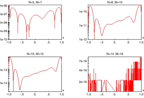
M increase the absolute errors get decreased.Finally, inTable 3the absolute errors obtained from the presented method are compared with the results obtained by the Chebyshev collocation method [9] for different values of N. From these data we can say that the presented method provides a better approximation when compared to Chebyshev collocation method [9].
Table 1
Numerical results of the exact solution and the approximate solutions ofExample 2for(N,M) = (8,10), (10,12).
xi Exact solution Approximate solution for N=8 Corrected approximate solution for
Approximate solution for N=10 Corrected approximate solution for y(xi) =exi y8(xi) y8,10(xi) y10(xi) y10,12(xi) Numerical solutions −1.0 0.367879441171 0.3678760382 0.367879441285 0.367879404465 0.367879441171 −0.6 0.548811636094 0.5488116259 0.548811636108 0.548811636168 0.548811636094 −0.2 0.818730753077 0.8187307911 0.818730753090 0.818730753505 0.8187307530780 0 1 1.0000000522 1.000000000016 1.000000000600 1.0000000000000 0.2 1.221402758160 1.2214028287 1.221402758182 1.221402758988 1.22140275816023 0.6 1.822118800390 1.8221189639 1.822118800427 1.822118802058 1.8221188003906 1.0 2.718281828459 2.7182878673 2.718281828526 2.718281883986 2.7182818284592 Table 2
Comparison of the absolute errors (actual, estimated, corrected) ofExample 2for(N,M) = (10,12), (14,16). xi Actual absolute errors
for N=10
Estimated absolute errors for N=10 and M=12
Corrected absolute errors for N=10 and M=12
e10(xi) e10,12(xi) E10,12(xi)
−1.0 0.364e−007 0.367e−007 0.147e−012
−0.6 0.542e−009 0.741e−010 0.436e−014
−0.2 0.818e−009 0.427e−009 0.325e−013
0 0.1e−008 0.600e−009 0.476e−013
0.2 0.137e−008 0.828e−009 0.671e−013
0.6 0.247e−008 0.166e−009 0.135e−013
1.0 0.563e−007 0.555e−007 0.227e−012
xi Actual absolute errors
for N=14
Estimated absolute errors for N=14 and M=16
Corrected absolute errors for N=14 and M=16
e14(xi) e14,16(xi) E14,16(xi)
−1.0 0.10e−009 0.13e−011 0.46e−018
−0.6 0.15e−010 0.57e−014 0.35e−019
−0.2 0.22e−010 0.13e−013 0.64e−019
0 0.75e−010 0.19e−013 0.91e−019
0.2 0.16e−009 0.26e−013 0.12e−018
0.6 0.40e−009 0.49e−013 0.21e−018
1.0 0.49e−009 0.16e−011 0.44e−018
Table 3
The comparison of the absolute errors obtained by the Chebyshev collocation method [9] and the presented method inExample 2.
N Presented method Method [9]
5 1.2e−006 2.23e−005
8 3.1e−010 8.27e−009
10 8.7e−013 3.25e−011
14 3.1e−018 1.06e−015
Example 3 ([6,10]). In this example, we solve the following Volterra integral equation of the second kind
y
(
x) +
xe−xy
1 2x
+
x 0 ex−ty(
t)
dt=
f(
x),
0≤
x≤
1.
1where f
(
x) = (
x+
1)
ex+
xe−12x. It can be easily obtained that the exact solution of this equation is y(
x) =
ex. Usingthe procedure in Section4the approximate solution yN
(
x)
and corrected approximate solutions yN,M(
x)
are calculated for(
N,
M) = (
3,
5), (
4,
6), (
5,
7)
and the findings are presented inTable 4. The numerical values of absolute error functions (actual, estimated and corrected) are compared for different values of N,
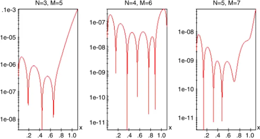
M inTable 5. From these data, it is noticed that the corrected absolute errors are closer to zero than actual absolute errors. Therefore, the corrected approximate solutions are quite close to exact solutions. Also, inTable 6the comparison of the absolute errors are obtained by the variational iteration method (VIM) [6], the Chebyshev polynomial method [10] and our method have been presented. As a result, we can say that our method gives better approximation than the others. InFig. 2, the orders of the corrected absolute errors with the increase of N,
M values have been examined.1e-06 1e-07 1e-08 1e-09 1e-10 -1.0 -.5 0. N=5, M=7 .5 1.0 1e-10 1e-11 1e-12 -1.0 -.5 0. N=8, M=10 .5 1.0 1e-13 1e-14 -1.0 -.5 0. N=10, M=12 .5 1.0 7e-16 4e-16 2e-16 -1.0 -.5 0. N=14, M=16 .5 1.0 x x x x
Fig. 1. Corrected absolute errors forExample 2.
Table 4
Numerical results of the exact solution and the approximate solutions ofExample 3for(N,M) = (4,6), (5,7). xi Exact solution Approximate solution for N=4 Corrected approximate solution for Approximate solution for N=5 Corrected approximate solution for y(xi) =exi y4(xi) y4,6(xi) y5(xi) y5,7(xi) Numerical solutions 0 1 1.0 1.0 1.0 1.0 0.2 1.221402758160 1.221418929924 1.221402817013 1.221399868181 1.2214027553169 0.4 1.491824697641 1.491807170607 1.491824677707 1.491821490146 1.4918246985692 0.6 1.822118800390 1.822377594578 1.822118822512 1.822181860977 1.8221187995560 0.8 2.225540928492 2.226490526881 2.225540912177 2.225974355345 2.2255409268373 1.0 2.718281828459 2.719653745069 2.718282077119 2.720777845559 2.7182818216242 1.1 3.004166023946 3.005062585901 3.004166083759 3.009290624488 3.0041659631211 Table 5
Comparison of the absolute errors (actual, estimated, corrected) ofExample 2for(N,M) = (4,6), (5,7). xi Actual absolute errors
for N=4
Estimated absolute errors for N=4 and M=6
Corrected absolute errors for N=4 and M=6
e4(xi) e4,6(xi) E4,6(xi)
0 0 0 0
0.2 0.16171764508e−004 0.16112911526e−004 0.5885298e−007
0.4 0.17527034040e−004 0.17507100761e−004 0.1993327e−007
0.6 0.25879418837e−003 0.25877206664e−003 0.2212172e−007
0.8 0.94959838946e−003 0.94961470399e−003 0.1631452e−007
1.0 0.13716679500e−002 0.13716679500e−002 0.2486605e−006
1.1 0.89650214214e−003 0.89650214214e−003 0.5981316e−007
xi Actual absolute errors
for N=5
Estimated absolute errors for N=5 and M=7
Corrected absolute errors for N=5 and M=7
e5(xi) e5,7(xi) E5,7(xi)
0 0 0 0
0.2 0.288997874775e−005 0.288713549287e−005 0.28432548e−008
0.4 0.320749515719e−005 0.320842315210e−005 0.92799490e−009
0.6 0.630605870487e−004 0.630614215242e−004 0.83447548e−009
0.8 0.433426852597e−003 0.433428507701e−003 0.16551041e−008
1.0 0.249601710031e−002 0.249602393508e−002 0.68347654e−008
N=3, M=5 .1e-3 1e-05 1e-06 1e-07 1e-08 .2 .4 .6 .8 1.0 x N=4, M=6 1e-07 1e-08 1e-09 1e-10 1e-11 .2 .4 .6 .8 1.0 x N=5, M=7 1e-08 1e-09 1e-10 1e-11 .2 .4 .6 .8 1.0 x
Fig. 2. Corrected absolute errors forExample 3.
Table 6
The comparison of the absolute errors obtained by the variational iteration method [6], Chebyshev collocation method [10] and the presented method inExample 3.
N Presented method Method [6] Method [10]
3 1.0e−004 4.6e−004 2.2e−004
4 3.0e−007 7.3e−007 9.2e−006
5 5.8e−008 1.1e−007 4.1e−007
Table 7
Numerical results of the exact solution and the approximate solutions ofExample 4for(N,M) = (8,10), (9,11). xi Exact solution Approximate solution for N=8 Corrected approximate solution for Approximate solution for N=9 Corrected approximate solution for y(xi) =Sin(x) y8(xi) y8,10(xi) y9(xi) y9,11(xi) Numerical solutions
0 0 0.166857e−004 0.173027e−008 0.2525237e−005 0.4359096e−010
0.2 0.1986693308 0.1986686537 0.1986693289 0.19867333711 0.19866933074
0.4 0.3894183423 0.3893930368 0.3894183398 0.38942267382 0.38941834224
0.6 0.5646424734 0.5646220969 0.5646424701 0.56464885284 0.56464247330
0.8 0.7173560909 0.7173209250 0.7173560861 0.71736503043 0.71735609076
1.0 0.8414709848 0.8414152532 0.8414709771 0.84148541445 0.84147098459
Example 4 ([11,16–18]). Our last example is the following Volterra–Fredholm integral equation x2y
(
x) +
exy(
2x) −
2x 0 ex+ty(
t)
dt+
1 0 ex−2ty(
2t)
dt=
f(
x)
where f(
x) = −
e4x−
1 4e x−2cos 2+
1 2e 3xcos 2x−
1 4e x−2sin 2−
1 2e3xsin 2x
+
x2sin x+
exsin 2x.The exact solution of this equation is y
(
x) =
sin(
x)
. The numerical results of this example are represented byTable 7. As you can see inTable 8the actual absolute errors, estimated absolute errors and corrected absolute errors are calculated for(
N,
m) = (
5,
7), (
8,
10), (
9,
11)
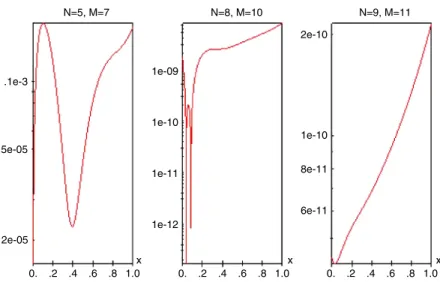
inTable 8. Additionally,Fig. 3shows the corrected absolute errors for different values ofN
,
M. When the findings which are obtained by Legendre collocation method in [11], Lagrange collocation method in [16] and Taylor collocation and matrix method in [17,18] are compared with the presented method, it is observed that the absolute errors of the presented method converge to zero rapidly for same values of N. You can see that inTable 9.8. Conclusion
In this study, to solve the Volterra type functional integral equations with variable bounds and mixed delay numerically, we introduce a matrix method depending on Taylor polynomials and collocation points. Also the residual correction procedure is given to estimate the absolute errors. The present method and the error analysis procedures are applied to some examples which have been solved by other methods in the literature. The method has advantages such as;
•
The present method is effective and by writing an algorithm in Maple 15, we can calculate the approximate solutions and absolute errors in short times.N=5, M=7 .1e-3 5e-05 2e-05 .2 0. .4 .6 .8 1.0 x N=8, M=10 1e-09 1e-10 1e-11 1e-12 x N=9, M=11 2e-10 1e-10 8e-11 6e-11 x .2 0. .4 .6 .8 1.0 0. .2 .4 .6 .8 1.0
Fig. 3. Corrected absolute errors forExample 4.
Table 8
Comparison of the absolute errors (actual, estimated, corrected) ofExample 4for(N,M) = (8,10), (9,11). xi Actual absolute errors
for N=8
Estimated absolute errors for N=8 and M=10
Corrected absolute errors for N=8 and M=10
e8(xi) e8,10(xi) E8,10(xi)
0 0.16685781624e−004 0.16684051351e−004 0.173027328082e−008
0.2 0.67702899078e−006 0.67514989359e−006 0.187909718729e−008
0.4 0.25305442864e−004 0.25302991432e−004 0.245143230119e−008
0.6 0.20376421549e−004 0.20373150372e−004 0.327117637004e−008
0.8 0.35165856326e−004 0.35161071778e−004 0.478454866545e−008
1.0 0.55731593897e−004 0.55723966844e−004 0.762705335039e−008
xi Actual absolute errors
for N=9
Estimated absolute errors for N=9 and M=11
Corrected absolute errors for N=9 and M=11
e9(xi) e9,11(xi) E9,11(xi)
0 0.252523777245e−005 0.252528136341e−005 0.4359096268288e−010
0.2 0.400632472238e−005 0.400637845105e−005 0.5372867348369e−010
0.4 0.433152051181e−005 0.433158913852e−005 0.6862670713931e−010
0.6 0.637944544234e−005 0.637953833336e−005 0.9289102012698e−010
0.8 0.893953385037e−005 0.893966879653e−005 0.1349461641220e−009
1.0 0.144296393900e−004 0.144298542965e−004 0.2149064882124e−009
Table 9
The comparison of the absolute errors obtained by the Taylor collocation [17], the Taylor matrix [18] methods, Lagrange collocation method [16], the Legendre collocation method [11] and the presented method inExample 4.
N Presented method Method [11] Method [16] Method [17] Method [18]
5 1.4e−004 2.93e−005 6.23e−005 6.23e−005 3.68e−004
8 7.4e−009 3.94e−008 1.77e−007 1.89e−008 1.24e−005
9 2.4e−010 2.29e−009 7.21e−006 2.35e−008 3.46e−007
•
As it is seen from the numerical examples, the method provides a better approximation than the all other methods such as the Legendre collocation method, the Lagrange collocation method, the Chebyshev collocation method, VIM method for different values of N.•
Even if the exact solution of the main problem is not known, the absolute errors are estimated with residual correction procedure.The method also can be developed and applied to differential functional integral equations with delay, nonlinear functional integral equations and functional integral equation systems.
References
[1]J. Banas, Z. Knap, Integrable solutions of a functional-integral equations, Rev. Mat. 2 (1) (1989) 31–38.
[2] T.L. Saaty, Modern Nonlinear Equations, New York, 1981.
[4] M. Kwapisz, J. Turo, Some integral-functional equations, Funkcial. Ekvac. 18 (1975) 107–162.
[5] S.N. Abskhabov, K.S. Mukhtarov, On a class of nonlinear integral equations of convolution type, Differ. Uravn. 23 (1987) 512–514.
[6] F. Bloom, Asymptotic bounds for solutions to a system of damped integro-differential equations of electromagnetic theory, J. Math. Anal. Appl. 73 (1980) 524–542.
[7] J. Biazar, et al., Numerical solution of functional integral equations by the variational iteration method, J. Comput. Appl. Math. 235 (2011) 2581–2585.
[8] M.T. Rashed, Numerical solutions of functional integral equations, Appl. Math. Comput. 156 (2004) 507–512.
[9] M.T. Rashed, Numerical solution of functional differential, integral and integro-differential equations, Appl. Math. Comput. 156 (2004) 485–492.
[10]E. Babolian, S. Abbasbandy, F. Fattahzadeh, A numerical method for solving a class of functional and two dimensional integral equations, Appl. Math. Comput. 198 (2008) 35–43.
[11]K. Maleknejad, S. Sohrabi, Y. Rostami, Numerical solution of nonlinear Volterra integral equations of the second kind by using Chebyshev polynomials, Appl. Math. Comput. 188 (2007) 123–128.
[12]S. Nemati, Numerical solution of Volterra–Fredholm integral equations using Legendre collocation method, J. Comput. Appl. Math. 278 (2015) 29–36.
[13]R. Firouzdor, A. Heidarnejad Khoob, Z. Mollaramezani, Numerical solution of functional integral equations by using B-splines, J. Linear Topol. Algebra 1 (1) (2012) 45–53.
[14]A.B. Tayler, Mathematical Models in Applied Mathematics, Clarendon Press, Oxford, 1986, pp. 40–53.
[15]M.A. Abdou, Fredholm–Volterra integral equation of the first kind and contact problem, Appl. Math. Comput. 125 (2002) 177–193.
[16]K.Y. Wang, Q.S. Wang, Lagrange collocation method for solving Volterra–Fredholm integral equations, Appl. Math. Comput. 219 (2013) 10434–10440.
[17]K. Wang, Q. Wang, Taylor collocation method and convergence analysis for the Volterra–Fredholm integral equations, J. Comput. Appl. Math. 260 (2014) 294–300.
[18]K. Maleknejad, Y. Mahmoudi, Taylor polynomial solution of high-order nonlinear Volterra–Fredholm integro-differential equations, Appl. Math. Comput. 145 (2003) 641–653.
[19]M. Sezer, Taylor polynomial solutions of Volterra integral equations, Internat. J. Math. Ed. Sci. Tech. 25 (5) (1994) 625–633.
[20]M. Gülsu, M. Sezer, Taylor collocation method for solution of systems of high-order linear Fredholm-Volterra integro-differential equations, Int. J. Comput. Math. 83 (4) (2006) 429–448.
[21]N. Kurt, M. Sezer, Polynomial solution of high-order linear Fredholm integro-differential equations with constant coefficients, J. Franklin Inst. 345 (8) (2008) 839.
[22]S. Yalçınbaş, M. Sezer, H. Sorkun, Legendre polynomial solutions of high-order linear Fredholm integro-differential equations, Appl. Math. Comput. 210 (2009) 334–349.
[23]B. Bülbül, M. Gülsu, M. Sezer, A new Taylor collocation method for non-linear Fredholm-Volterra integro-differential equations, J. Numer. Methods Partial Differential Equations 26 (2010) 1006–1020.
[24]S. Yalçınbaş, M. Aynigül, M. Sezer, A collocation method using Hermite polynomials for approximate solution of pantograph equations, J. Franklin Inst. B 348 (2011) 1128–1139.
[25]E. Gokmen, M. Sezer, Taylor collocation method for systems of high-order linear differential–difference equations with variable coefficients, Ain Shams Eng. J. 4 (1) (2013) 117–125.
[26]E. Gokmen, O.R. Isik, M. Sezer, Taylor collocation approach for delayed Lotka–Volterra predator–prey system, Appl. Math. Comput. 268 (2015) 671–684.
[27]E. Gokmen, M. Sezer, Approximate solution of a model describing biological species living together by Taylor collocation method, New Trends Math. Sci. 3 (2) (2015) 147–158.
[28]G. Yuksel, Ş. Yuzbasi, M. Sezer, A Chebyshev method for a class of high-order linear Fredholm integro-differential equations, J. Adv. Res. App. Math. 4 (2012) 49–67.
[29]F.A. Oliveira, Collocation and residual correction, Numer. Math. 36 (1980) 27–31.
[30]I. Celik, Approximate calculation of eigenvalues with the method of weighted residuals–collocation method, Appl. Math. Comput. 160 (2005) 401–410.
[31]S. Shahmorad, Numerical solution of the general form linear Fredholm–Volterra integro-differential equations by the Tau method with an error estimation, Appl. Math. Comput. 167 (2005) 1418–1429.