Journal of Applied Fluid Mechanics, Vol. 14, No. 1, pp. 23-36, 2021.
Available online at
www.jafmonline.net
, ISSN 1735-3572, EISSN 1735-3645.DOI: 10.47176/jafm.14.01.31475
An Investigation of Transition Flow in Porous Media by
Event Driven Molecular Dynamics Simulation
M. Koc
1†, I. Kandemir
2and V. R. Akkaya
31 Istanbul Arel University Vocational School Machine Program, Kucukcekmece, Istanbul, 34295, Turkey 2Gebze Technical University Faculty of Engineering Department of Mechanical Engineering
Cayirova, Kocaeli, 41400, Turkey
3Mugla Sitki Kocman University Faculty of Technology Department of Energy Systems Engineering, Mentese,
Mugla, 48000, Turkey
†Corresponding Author Email: [email protected] (Received February 13, 2020; accepted July 1, 2020)
A
BSTRACTAim of this study is to investigate the properties of mono-atomic gas flow through the porous medium by using Event-Driven Molecular Dynamics (EDMD) simulation in the transition regime. The molecules and the solid particles forming the porous structure were modelled as hard spheres hence molecule trajectories, collision partners, interaction times and post-collision velocities were calculated deterministically. The porous medium is formed of spherical particles suspended in the middle of the channel and these particles are distributed into the channel in a regular cubic array. Collisions of gas molecules with porous medium were provided by means of the specular reflection boundary condition. A negative pressure boundary condition was applied to the inlet and outlet of the porous media to ensure gas flow. Porosity, solid sphere diameter and Knudsen number (Kn) were initially input to the simulation for different Cases. Thus, the effects of these parameters on mass flow rate, dynamic viscosity, tortuosity and permeability were calculated by EDMD simulation. The results were compared with the literature and were found to be consistent.
Keywords: Event driven molecular dynamic simulation; Knudsen Number; Porosity; Tortuosity; Permeability; Viscosity; Mass flow rate; Transition regime; Darcy’s law; Klinkenberg’s theory.
NOMENCLATURE 𝑑𝑚 molecular diameter
𝐷𝑝 pore diameter
𝐷𝑠𝑜𝑙 diameter of a solid sphere 𝑓 collision frequency 𝐾 permeability 𝐾𝑎𝑝𝑝 apparent permeability 𝐾𝑖𝑛𝑡 intrinsic permeability 𝐾𝑛 Knudsen number
𝐿𝑎𝑐𝑡 average length of the devious path 𝐿𝑝𝑚 length of the porous medium 𝐿𝑇 total distance
𝑚𝑚𝑜𝑙 mass of a single molecule 𝑁𝑐 Total number of collisions 𝑁𝑖𝑛 Number of molecules entering 𝑁𝑜𝑢𝑡 Number of molecules exiting
𝑝 pressure
𝑃𝑖𝑛 momentum of incoming molecule 𝑃𝑟𝑒𝑓 momentum of reflected molecule 𝑠 center-to-center distance
𝑆𝑠𝑜𝑙 total surface area of solid particles 𝑡𝑖𝑛 entry time 𝑡𝑜𝑢𝑡 exit time 𝑢𝑚𝑎𝑔 magnitude of velocity 𝑢𝑥 flow velocity 𝜀 porosity 𝛥𝑝 pressure difference 𝛥𝑡 time interval 𝜆 mean free path 𝜇 dynamic viscosity 𝜏 tortuosity
1. INTRODUCTION
Flow in porous media is an essential research area for
many science and engineering fields. Porous media are particularly used in micro-sized device like channels, nozzles, pumps for micro filtration,
fractionation, and catalysis applications. In such applications, porous media is in nano scale. Experimental possibilities for gas transport in such media are very limited. In devices such as proton exchange membrane fuel cells, the pores of the porous medium are even smaller than the mean free path of the molecules (Kawagoe et al. 2016; Jeong et
al. 2006). For this reason, the transition regime, the most important Kn-related regime, was examined in this study.
To understand Kn-related gas flow regime in porous media, one needs to define Kn which is the ratio of the mean free path to the pore diameter (𝜆/𝐷𝑝). From kinetic theory, mean free path perspective is given by 𝜆 =√2𝜋𝑑1
𝑚
2𝑛 (1)
where 𝑛 is the number density, 𝑑𝑚 is the molecular diameter.
In the continuum flow regime, where Kn is less than 0.001, pore size is greater than the mean free path of the molecule. In this regime, the velocity of the molecule on the solid surface is assumed to be zero and intermolecular collisions are dominant. Slip regime is observed when the pore size is about the same size as the mean free path of the molecule. Velocity on the solid surface is greater than zero in this regime and Kn varies from 0.01 to 0.1. As Kn increases to between 0.1 and 10, pore size becomes smaller than the mean free path of the molecule. This region is called the transition regime and exhibits a flow characteristic between slip and molecular flow regime. Gas molecules move between the pores more individually than a bulk fluid motion, and collisions between molecules and porous medium prevail over intermolecular collision. In the molecular flow regime where Kn is greater than 10, intermolecular interaction is negligible.
Molecular interaction-based methods such as Molecular Dynamics (MD), Direct Simulation Monte Carlo (DSMC) and Lattice Boltzmann Method (LBM) are used since the Navier-Stokes (N-S) method is no longer valid.
Permeability is determined as the ability of the porous medium to allow the passage of fluid through it and it is one of the most important porous media flow parameters (Ezzatabadipour and Zahedi 2018). It is an important feature for most practical applications in terms of mass transfer and fluid flow characterization in porous media. Therefore, an accurate calculation is highly vital to determine flow properties and quality of the porous structure (Chen and Yao 2017).
Permeability of a porous medium measured in the non-slip and laminar flow depends only on the structure of the medium and known as intrinsic permeability. In this regime, Darcy's law (Darcy 1856) is the most commonly used method for predicting permeability. Pressure difference, fluid viscosity and flow rate applied in Darcy's law are discussed. Laminar flow through a homogeneous porous medium dominated by viscous effects is generally Darcy's law and calculated as
−𝐿𝛥𝑝
𝑝𝑚=
𝜇0
𝐾𝐷𝑢 (2)
Here, 𝛥𝑝 is the pressure difference across length of the porous medium 𝐿𝑝𝑚, velocity corresponding to
the volumetric fluid discharge 𝑢 and dynamic viscosity of the fluid 𝜇0 (Darcy 1856). SI unit for permeability is m2.
However, the situation for the permeability shown for gases is slightly different. In the same porous structure, permeability value starts to increase as Kn is relatively high. The effect of Kn in porous media was first studied by Klinkenberg (1941). It has been shown in many studies that measured (apparent) permeability is higher than intrinsic permeability measured in viscous flow due to Kn effect and this difference increases with increasing Kn.
In the Klinkenberg model, it is predicted that permeability is pressure dependent and relationship between apparent permeability and intrinsic permeability (continuous regime) is provided by 𝐾𝑎𝑝𝑝= 𝐾𝑖𝑛𝑡(1 +𝑏𝑃) (3) Florence et al. (2007) corrected this expression according to kinetic theory as follows
𝐾𝑎𝑝𝑝= 𝐾𝑖𝑛𝑡(1 + 4𝑐𝐾𝑛) (4)
Here, c ratio factor or Maxwell slip coefficient is generally chosen at 1 or slightly below. Beskok and Karniadakis (1999), who argued that Kn would be more important in a much narrower pore size, proposed an experimental model for Klinkenberg's linear correction.
𝐾𝑎𝑝𝑝= 𝐾𝑖𝑛𝑡[1 + 𝛼𝐾𝑛 (1 +1+𝐾𝑛4𝐾𝑛)] (5) Where 𝛼 = 128/15𝜋2+ 𝑡𝑎𝑛−1(4𝐾𝑛0.4). Ho et al. (2019) correlated the experimental constant with the mass flow rate 𝛼 = 1.358/(1 + 0.178𝐾𝑛−0.4348) . In the study of Yu and Cheng (2002), Kozeny-Carman equation (Kozeny 1927; Kozeny-Carman 1997) for the porous media consisting of spherical solid particles (mono-dispersed porous medium) are given by the following equation
𝐾𝐾−𝐶= 𝜀
3𝐷
𝑠𝑜𝑙2
180(1−𝜀)2 (6)
Where 𝐷𝑠𝑜𝑙 is diameter of solid sphere. The K-C equation for both cubic and triangular sphere particles was reconsidered by Chen and Yao (2017) and expressed as
𝐾𝐾−𝐶=35(3+2√2)𝑘8 ⋅ 𝜀
2
1−𝜀𝐷𝑝
2 (7)
where pore diameter is 𝐷𝑝=12[𝐷𝑠𝑜𝑙√1−𝜀𝜀 +𝐷𝑠𝑜𝑙
2 √2 ( 1
(1−𝜀)− 1)] , 𝐷𝑠𝑜𝑙 is diameter of solid sphere and k = 5 for uniform sphere particles. In the study of Yu and Cheng (2002), the maximum pore diameter is given by 𝐷𝑝= 𝐷𝑠𝑜𝑙√2𝜀/(1 − 𝜀)/2 for bi-dispersed dispersed porous structure with triangular array. Wu and Yu (2007) proposed 𝐷𝑝= 𝐷𝑠𝑜𝑙(√𝜀/(1 − 𝜀) +
√𝜋 ∕ 4(1 − 𝜀) − 1)/2 for square particle array. In addition, Ergun (1952) presented the following model:
𝐾𝐸= 𝜀
3𝐷
𝑠𝑜𝑙2
150(1−𝜀)2 (8)
All permeability models given so far apply to continuum flow regime. Mostafavi et al. (2017) proposed relation given in eq. (9), which also depends on Kn, for the porosity calculation of the porous structure formed by in-line arrangement of square particles.
𝐾𝑀= 𝐴 [(1−𝜀)𝜀3 2]
𝐵
𝐷𝑠𝑜𝑙2 (9)
Where 𝐴 = 0.00077795𝐾𝑛 + 0.024 , 𝐵 = 0.0006989𝐾𝑛 + 0.4979 and 𝐷𝑠𝑜𝑙 is the diameter of a particle. Koponen et al. (1998) and Tomadakis & Robertson (2005) obtained effect of change of fiber diameter on permeability for viscous flow in fiber-structured porous media. Davies (1952) proposed a permeability calculation for flow within the fibrous structure with the help of an empirical correlation, including porosity and fiber diameter. In the study of Yang and Weigand (2018), where the Klinkenberg effect is investigated, the pressure-driven gas flow characteristics through a porous medium was examined in the slip and transition regime with the help of the DSMC method.
Another important parameter to understand the structure of porous medium and its effects on flow is tortuosity. This concept, unlike measurable concepts such as porosity and pore size, allows the determination of flow paths, which are mostly connected to the porous structure. This allows us to understand how devious streamline of the fluid is in the porous medium. It is defined as ratio of average length of this devious path of gas molecules through the porous structure to length of the porous medium in the flow direction.
𝜏 =𝐿𝑎𝑐𝑡
𝐿𝑝𝑚 (10)
There are many models in literature for calculating tortuosity. Some of them evaluated tortuosity only in terms of its dependence on porosity. The well-known model (Bruggeman 1935) proposed the following equation for composite heterogeneous randomly dispersed solid particles
𝜏𝐵= 𝜀1−𝛼 (11) Here α the base of Bruggeman and is assumed to be 1.5 for sphere in standard form and 2 for cylinder (Tjaden et al. 2018), but Bruggeman used this value to describe specific structures containing dispersed particles. Comiti and Renaud (1989) proposed a model for tortuosity in experimental studies on flow in spherical and cubic particle media.
𝜏𝐶𝑅= 1 + 𝑝 𝑙𝑛 (1𝜀) (12)
Here, 𝑃 is an experimental value and 0.63 is given for cubic particles. Pisani (2011) proposed the following model to demonstrate porosity dependence of tortuosity in a porous structure composed of spheres.
𝜏𝑃= 1 + 𝛼(1 − 𝜀) (13)
Here α is the shape factor and 0.75 is taken for the spheres. Vallabh et al. (2010) studied experimentally relationship between media properties such as porosity, fiber diameter, and tortuosity in a porous medium consisting of a fiber network. In addition, Tomadakis and Sotirchos (1993) studied tortuosity in the medium of randomly distributed and overlapping capillary channels. Shariati et al. (2019) investigated effects of porosity and solid particle diameter on porosity of random spheres and relationship between Kn and tortuosity.
Dynamic viscosity of gases differs from that of liquids and is highly dependent on the Kn. Beskok and Karniadakis (1999) calculated the following equation with the help of the numerical calculations of the flow through cylinder and N-S equations by implementing slip condition in order to find out how effective (measured) viscosity changes with Kn.
𝜇𝑒,𝐵𝐾= 𝜇01+𝑎𝐾𝑛1 (14)
Here, 𝜇0 is viscosity at continuous limit without slip effect. In the flow simulation by Michalis et al. (2010) using DSMC with a hard sphere gas model, the factor 𝑎 is given by the ratio of the length of the porous medium to the width 𝐿/𝐻 . According to Beskok and Karniadakis (Beskok and Karniadakis 1999), 𝑎 is not a constant but depends on Kn. Kn in the equation was found by the ratio of the mean free path to the width of the medium (Kalarakis et al. 2012). Guo et al. (2006) calculated dependence of effective viscosity on Kn for the flow of the transition regime in a microchannel with the following equation.
𝜇𝑒,𝐺=2𝜇0
𝜋 𝑎𝑟𝑐𝑡𝑎𝑛(√2 𝐾𝑛
−3/4) (15) Sutherland (1905) used hard sphere intermolecular potential approach for calculation of viscosity. Hadjiconstantinou (2003) modified Cercignani's second order slip model and solved the Boltzmann equation for hard sphere gas for a wide range of rarefaction. It obtained dependence of flow rate on Kn. Cercignani et al. (2004) applied different techniques to Boltzmann equation to obtain gas flow rate in the microchannel. Guo et al. (2008) obtained the generalized lattice Boltzmann equation technique and the Poiseuille flow mass flow rate dependence on Kn. Dadzie and Brenner (2012) examined mass flow rate in pressure-driven flow in the transition regime with different non-kinetic approaches and experimental observations. Danielewski and Wierzba (2010) described several partial differential equation aid diffusion-mediated mass transfers based on Bi-velocity (Darken) method. Dongari et al. (2009) obtained modified N-S equations by adding extra diffusion terms and examined the effect of Kn on mass transfer in pressure gradient-induced flow. Beskok and Karniadakis (1999) developed a simple physics-based model and estimated the mass and volume flow rate in the channel flow over the whole Kn range.
Molecular Dynamics (MD) and Direct Simulation Monte Carlo (DSMC) methods are the most
important simulation methods based on interaction of molecules with each other and boundaries. In molecular dynamic simulations, computational difficulties arise as number of molecules grows, because the interactive particles and their position must be calculated for each interaction. The DSMC method (Bird 1994) uses several representative molecules to simulate a larger number of actual molecules. The movements of molecules are precise, but collisions are likely to be produced. On the other hand, MD simulations are much more realistic and accurate because each particle represents a real molecule and its position and velocity are fully known. It includes algorithms suitable for the integration of Newton's equation of motion for many time steps for systems with multiple particles because of its time-driven nature. Main disadvantages of standard MD simulations based on continuous interaction potential (the most widely used is Lennard-Jones potential) are limitations of simulation time and size. Integration time step is so small that, during a ten-micro-second simulation, even ten thousand molecules representing a very small volume require too many time steps and a crash test at each step. Thanks to hard sphere assumption in which interaction potential is considered discrete (zero except at moment of contact), collision times can be predicted analytically and allows the simulation to be handled as series of asynchronous events. This is called Event Driven Molecular Dynamics (EDMD) simulations and enables simulation of larger systems for longer periods than time-driven simulations. This approach has been shown to produce consistent results in the calculation of transport coefficients for rarefied gases (Kandemir 1999; Greber et al. 2001; Akkaya and Kandemir 2015). Unlike DSMC, molecule trajectories, determination of collision pairs and post collision velocities the molecules to collide and the calculation of post-collision velocities are calculated deterministically in EDMD. In addition, all collisions are real and predictable, no collision is omitted. Since the first introduction of EDMD simulations (Alder and Wainwright 1957), the developments of more effective algorithms have further improved performance of EDMD (Rapaport 1980; Kandemir 1999; Donev et al. 2008). With the computational power of a desktop computer, simulation of millions of particles is possible for longer periods (Bannerman et al. 2011). Another advantage of EDMD method is that it is as deterministic as other classical MD methods and allows working with as many molecules as the DSMC method. Rather than relying on data from very few molecules simulated as in DSMC, it uses the entire simulation domain as physical domain, considering all molecules in this physical domain as real molecules, and all interactions as real interactions. Thanks to the mentioned assumptions and improvements in EDMD, computing performance can compete with DSMC.
In this study, the flow of monoatomic Ar gas in porous medium was investigated by EDMD simulation. With EDMD simulation, gas flow properties directly connected to porous structure were obtained spontaneously without the need for
any macroscopic equation. Most of the EDMD simulation results were compared with the literature and found to be quite compatible.
2. EDMD METHOD AND DETAILS
The molecules obey Newton's laws of motion in EDMD simulations. The molecules collide if their trajectories intersect: ∑ (𝑥𝑗,𝑘∗ − 𝑥𝑖,𝑘∗ ) 2 3 𝑘=1 = (ⅆ𝑚,𝑗+ⅆ𝑚,𝑖)2 4 (16) Here 𝑖 and 𝑗 denote the pair of the molecules to collide, 𝑥𝑘∗ position component, 𝑑 is diameter of the molecules. Given that a separate time variable (𝑡𝑖, 𝑡𝑗) is held for each molecule in the EDMD, the positions of the molecules at the moment of collision are calculated from the following formula:
𝑥𝑖,𝑘∗ = 𝑥𝑖,𝑘+ 𝑐𝑖,𝑘(𝑡 − 𝑡𝑖) 𝑥𝑗,𝑘∗ = 𝑥
𝑗,𝑘+ 𝑐𝑗,𝑘(𝑡 − 𝑡𝑗) (17) where 𝑐𝑘 is velocity component. If the values in Eq. (19) are substituted in Eq. (18), the following equation is obtained: ∑ (𝑥𝑖,𝑘+ 𝑐𝑖,𝑘(𝑡 − 𝑡𝑖) − 𝑥𝑗,𝑘− 𝑐𝑗,𝑘(𝑡 − 𝑡𝑗)) 2 = 3 𝑘=1 𝑑2 (18) To get Eq. (20) to a simpler form, 𝛥𝑥𝑘 and 𝛥𝑐𝑘 are defined:
𝛥𝑥𝑘= 𝑐𝑗,𝑘𝛥𝑡𝑖,𝑗+ 𝑥𝑗,𝑘− 𝑥𝑖,𝑘
𝛥𝑐𝑘= 𝑐𝑗,𝑘− 𝑐𝑖,𝑘 (19) So Eq. (20) would be as follows:
∑3 (𝛥𝑐𝑘)2(𝑡 − 𝑡𝑖)2
𝑘=1 + 2𝛥𝑥𝑘𝛥𝑐𝑘(𝑡 − 𝑡𝑖) +
(𝛥𝑥𝑘)2= 𝑑2 (20) If 𝐴 = ∑3𝑘=1(𝛥𝑐𝑘)2, 𝐵 = ∑3𝑘=1𝛥𝑥𝑘𝛥𝑐𝑘 and 𝐶 = ∑3 (𝛥𝑥𝑘)2
𝑘=1 − 𝑑2 are defined for a simpler representation, the collision time is presented in quadratic form as:
𝐴(𝑡 − 𝑡𝑖)2+ 2𝐵(𝑡 − 𝑡𝑖) + 𝐶 = 0 (21) If the trajectories do not intersect, this equation has no real root. If there are positive real roots, the smaller value gives the collision time of the molecule pair.
Deterministically predictable collision times allow the simulation to be divided into a series of asynchronous events. This process is event-driven, since the simulation time can skip from one event to another.
In the initialization of the simulation, since the boundary temperatures of the channel are the same and constant inside the channel, after a certain period of time, thermal equilibrium occurs for every point of the channel. Monoatomic molecules only have a translation energy mode. In the case of thermal equilibrium, there is a relationship between the kinetic temperature and the average translational
kinetic energies of molecules as follows. 3
2𝑘𝑏𝑇 = 1
2𝑚⟨𝑐2⟩ (22) where ⟨𝑐2⟩ is the average of thermal velocity squares of molecules. The kinetic theory says that in a system with thermal equilibrium, molecules will have a velocity distribution determined by the Boltzmann distribution. The most probable speed according to this distribution is as follows.
𝑐𝑚𝑝= √23⟨𝑐2⟩ (23) Thus, the thermal velocity components sampled from the distribution are as follows.
𝑢𝑡ℎ= 𝑐𝑚𝑝√−𝑙𝑛(𝑅1) sin(2𝜋𝑅2) 𝑣𝑡ℎ= 𝑐𝑚𝑝√−𝑙𝑛(𝑅3) sin(2𝜋𝑅4)
𝑤𝑡ℎ= 𝑐𝑚𝑝√−𝑙𝑛(𝑅5) sin(2𝜋𝑅6) (24) In this study using EDMD simulation, monoatomic molecules are modeled as hard spheres. The potential for interaction between hard particles is discrete; that is, no force is applied other than the instantaneous, binary collision of molecules. Assuming there is no external force field, the resulting trajectories are linear and molecular velocity between the two collisions is constant. When a collision occurs, post-collision velocities are determined analytically by conservation of energy and momentum. The type of molecule pair that participates in the collision determines the collision characteristic. In this monoatomic MD study, intermolecular collisions are elastic. In collisions of this type, mass, translational energy and momentum are conserved.
𝑚𝐴+ 𝑚𝐵= 𝑚𝐴′ + 𝑚𝐵′ 𝑚𝐴𝑐𝐴+ 𝑚𝐵𝑐𝐵= 𝑚𝐴′𝑐𝐴′+ 𝑚𝐴′𝑐𝐵′
𝑚𝐴|𝑐𝐴|2+ 𝑚𝐵|𝑐𝐵|2= 𝑚𝐴′|𝑐𝐴′|2+ 𝑚𝐴′|𝑐𝐵′|2 (25) where ′ indicates post-collision situations. 𝑚 and 𝑐 indicate mass and velocity of the molecule, respectively. Accordingly, the post-collision velocities of the molecule pair are expressed as follows. 𝑐𝐴′ = 𝑐𝐴− 2𝜇𝐴𝐵 𝑚𝐴 𝜖⟨𝜖, 𝑐𝐴− 𝑐𝐵⟩ 𝑐𝐵′ = 𝑐𝐵−2𝜇𝐴𝐵 𝑚𝐴 𝜖⟨𝜖, 𝑐𝐴− 𝑐𝐵⟩ (26)
Here the inner product is shown as ⟨⋅,⋅⟩. 𝜇𝐴𝐵 is reduced mass and 𝜖 is the unit vector passing through the molecule centers at the moment of contact.
𝜇𝐴𝐵= 𝑚𝐴𝑚𝐵
𝑚𝐴+𝑚𝐵 𝜖 =
𝑥𝐴−𝑥𝐵
|𝑥𝐴−𝑥𝐵| (27)
The collision of molecules with solid spheres follows the same rules. But, since the mass of the solid sphere is considered as infinitely large, the collision is like a molecule colliding with a stationary sphere. So the velocity of the solid sphere before and after the collision is zero. Thus the specular reflection condition is also achieved for spherical particles.
EDMD simulation was performed by the real number cell division method. One cell has 26 adjacent cells in 3D. In this method, each molecule is placed in a cell according to its position. Thus, the most likely collisions’ pair of molecules at a given time is only molecules in a cell or adjacent cells. This multi-cell method can therefore ensure that no collisions are missed. The events in the EDMD simulation are intermolecular collisions, molecule-boundary interaction and crossing from a cell to another. The main purpose is to find the earliest event and simulate it. For this purpose, the technique of dividing into cells, the use of priority queues for event sequencing Paul (2007) and Marín and Cordero (1995) that Akkaya and Kandemir (2015) implemented in EDMD are more advantageous both in accuracy and reducing the computational effort to
O(1) for EDMD simulations. For data reduction, the
calculation domain was divided into small sub-domains (bins), and by taking the average of the snapshots of these bins at certain intervals, profiles of the basic properties of the fluid were obtained. In order to simulate a confined gas flow using molecular simulations, system boundaries and interactions with gas molecules must be appropriately modeled. Three types of boundaries are generally sufficient to represent a flow in a micro or nano channel. These well-known boundaries are periodic, wall and flow boundaries. In the presence of periodic boundaries simulation domain is modelled as an infinite lattice by repeating the calculation region along the boundary direction. When a molecule reaches a periodic boundary, it leaves the domain and enters from the exact opposite side again while keeping its velocity. When a molecule reaches the wall boundary, it is reflected back with a new velocity determined by the wall model. Specular reflection used in this study is the most basic wall model where the surface is perfectly smooth at the molecular level. When a molecule undergoes specular reflection, the tangential components remain unchanged, while the normal velocity component, which maintains the tangential momentum, is reversed. In fact, however, the wall surface is rough, and molecules are projected at random angles from the wall. Diffuse reflection is the most common model representing these surfaces. In the common model, the post-reflection rate of the molecule is largely independent of the incoming velocity and is stochastically determined from a distribution based on wall temperature and velocity.
The implicit treatment method is first introduced for DSMC simulations by Liou and Fang (2000) and adapted for EDMD simulations by Akkaya and Kandemir (2015). In this study, implicit treatment method is one of the flow boundary conditions developed to create a flow within the channel molecules reaching both ends of the system (upstream or downstream) leave the computational domain permanently. New molecules are inserted into the computational domain according to local domain properties. For both flow boundaries, the molecular flux entering the calculation domain is
determined by the Maxwell distribution function: 𝐹𝑗=2√𝜋𝛽𝑛𝑗 𝑗[ⅇ −𝑠𝑗2𝑐𝑜𝑠2𝜙 + √𝜋𝑠𝑗𝑐𝑜𝑠 𝜙 (1 + ⅇ𝑟𝑓(𝑠𝑗𝑐𝑜𝑠 𝜙))] (28) where 𝑠𝑗= 𝑈𝑗𝛽𝑗, 𝛽𝑗= 1/𝑐𝑚𝑝,𝑗= 1/√2𝑘𝑏𝑇𝑗∕ 𝑚 Here, 𝑈 , 𝑇 , 𝑛𝑗 and 𝑐𝑚𝑝 are streamwise velocity, local temperature, number density of molecules in the cell and the most probable speed, respectively. This molecular flux should be calculated for each cell surface of each flow boundary cell 𝑗. The value of 𝜙 is 0 for upstream and 𝜋 for downstream. The number of molecules entering the calculation domain from the cross-sectional area (A) of the boundary surface per unit time (𝛥𝑡 ) gives the following relation:
𝑁𝑖𝑛,𝑗 = 𝐹𝑗𝛥𝑡𝐴𝑗 (29) The tangential velocity components (𝑣 and w) of the incoming molecules that are independent of streamwise are produced as follows:
𝑣 = 𝑉 + 𝑐𝑚𝑝𝑅𝑛
√2 𝑤 = 𝑊 + 𝑐𝑚𝑝 𝑅𝑛′
√2
(30) Here, 𝑉 and 𝑊 are mean tangential velocity components, and 𝑅𝑛 and 𝑅𝑛′ are random numbers generated from normal distribution with zero mean and unit variance.
If the streamwise velocity 𝑈 = 0, normal component becomes
𝑢 = 𝑐𝑚𝑝√−𝑙𝑜𝑔𝑅𝑢 (31) Here, 𝑅𝑢 is random number generated from uniform distribution of interval [0,1). For 𝑈 ≠ 0, Garcia and Wagner (2006) introduce several efficient acceptance-rejection methods with the general form of
𝑢 = 𝑈 − 𝑓 (𝑐𝑈
𝑚𝑝) 𝑐𝑚𝑝 (32)
Here, 𝑓(𝑈/𝑐𝑚𝑝) is a random number selected through an acceptance-rejection method. In this study, recommended method for low speed flows (-0.4𝑐𝑚𝑝< 𝑈<1.3𝑐𝑚𝑝) was used.
The inlet pressure (𝑝𝑖𝑛) and temperature (𝑇𝑖𝑛) are known for the upstream boundary. 𝑉𝑖𝑛 and 𝑊𝑖𝑛 are set to zero. The molecular number density is calculated from the ideal gas equation:
𝑛𝑖𝑛=𝑘𝑝𝑖𝑛
𝑏𝑇𝑖𝑛 (33)
Streamwise velocity perpendicular to the surface is expressed as a function of the mean flow velocity (𝑈𝑗), pressure (𝑝𝑗), density (𝜌𝑗) and sound velocity (𝑎𝑗) of the computational domain:
(𝑈𝑖𝑛)𝑗= 𝑈𝑗+ 𝑝𝑖𝑛−𝑝𝑗
𝜌𝑗𝑎𝑗 (34)
Only the outlet pressure (𝑝𝑒) is known at the downstream boundary. Other flow properties are calculated by extrapolating from neighbor cell:
(𝑛𝑒)𝑗= 𝑛𝑗+ 𝑝𝑒− 𝑝𝑗 (𝑎𝑗)2 (𝑈𝑒)𝑗= 𝑈𝑗+ 𝑝𝑗− 𝑝𝑒 𝜌𝑗𝑎𝑗 (𝑇𝑒)𝑗= −(𝑛𝑝𝑒 𝑒)𝑗𝑘𝑏 (35)
The tangential components of the average flow velocity components are calculated similarly for the upstream:
(𝑉𝑒)𝑗= 𝑉𝑗 (𝑊𝑒)𝑗= 𝑊𝑗
(36) Unlike the classical MD, there is no need for temperature and pressure control or use of any thermostat like Berendsen or Nose-Hoover in this method. No macroscopic information, except for the initial conditions and boundary conditions, is imposed on the system. Macroscopic properties develop spontaneously throughout the simulation. Defining the fluid as an ensemble of molecules allows all macroscopic features of the system to be calculated from the instantaneous velocity, position and energy information of each molecule. The number of molecules included in the calculation domain from the flow boundary and the velocity of these molecules are determined by the local flow properties such as temperature, pressure, molecular density and average velocity.
3. CALCULATIONS IN EDMD
SIMULATIONS
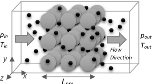
The sample channel with porous medium is shown schematically in Fig. 1. Our nano / micro channel is 3-dimensional (x, y, z axis) and has a rectangular cross-section. The calculation for flow parameters is only for porous media volume. Interactions between molecules and solid particles are modeled by specular reflection condition. Periodic boundary condition is applied to y and z axes. The flow is along the x-axis. The pressure boundary condition mentioned in section 2 was applied. Under this condition, only the pressure and temperature input are entered. Statistically, influx is calculated per unit time and molecules are added to the system (upstream). When the flow occurs, the molecules exit the system spontaneously create outflux (downstream).
In order to form a porous medium, equal-sized solid spherical particles are placed in a cubic arrangement in the middle of a rectangular channel. During the simulation, masses of these particles assigned infinite and their velocity is zero. The apertures between the spheres were calculated for each porosity value.
Structures consisting of interconnected pores, such as our porous structure, have effective porosity. If there is a gap between the particles forming the pore, normal porosity and effective porosity are equal to each other (Kaviany 1966). Therefore, the porosity for this study was defined by the ratio of void volume to the total volume of void and solid particles. 𝜀 = 𝑉𝑣𝑜𝑖𝑑
𝑉𝑣𝑜𝑖𝑑+𝑉𝑠𝑜𝑙 (37)
velocity components in the flow direction of the molecules in the medium and number of molecules entering and exiting the medium unit time are calculated by means of expression
𝐾𝑠𝑖𝑚=𝐿𝑝𝑚 ∑𝑛=𝑁𝑚𝑛=1 𝑢𝑥 𝑁𝑚 𝑁𝑜𝑢𝑡+𝑁𝑖𝑛 2𝛥𝑡 (38)
by EDMD simulation and averaged at each Δt time interval. Where (𝑁𝑜𝑢𝑡+ 𝑁𝑖𝑛)/2𝛥𝑡 is the average number of molecules exiting and entering the medium at a given time interval, ∑𝑛=𝑁𝑛=1𝑚𝑢𝑥/𝑁𝑚 mean of the velocity components in the flow direction of all passing molecules and 𝐿𝑝𝑚 is the length of the porous media.
Fig. 1. Schematic representation of channel structure with the porous medium (Greys represent solid spheres forming the porous medium and blacks represent monoatomic
Argon).
In this study, Newton's law of motion is used for calculating tortuosity. By keeping the entry and exit times of gas molecules in porous medium, we can find the average path lengths of molecules in the medium by taking ⟨∑𝑡𝑜𝑢𝑡− 𝑡𝑖𝑛⟩ multiplying the average velocity of the molecules in the medium by ⟨∑𝑢𝑚𝑎𝑔⟩. In this context, if we apply the definition of tortuosity to EDMD simulation, we get the expression 𝜏𝑠𝑖𝑚=⟨∑𝑡𝑜𝑢𝑡−𝑡𝑖𝑛⟩⟨∑𝑢𝑚𝑎𝑔⟩ 𝐿𝑝𝑚 (39) and ⟨∑𝑢𝑚𝑎𝑔⟩ = ∑𝑛=𝑁𝑚√𝑢𝑥2+ 𝑢𝑦2+ 𝑢𝑧2 𝑛=1 /𝑁𝑚.
In Kandemir (1999) study, the model developed for Shear-Driven Couette flow for viscosity calculation from the molecular dynamics perspective was applied to flow in porous media;
𝜇𝑠𝑖𝑚=
𝐿𝑇,𝑚𝑜𝑙−𝑠𝑜𝑙 𝑁𝑐,𝑚𝑜𝑙−𝑠𝑜𝑙𝛴〈𝑃𝑖𝑛−𝑃𝑟𝑒𝑓〉
⟨∑𝑢𝑚𝑎𝑔⟩𝑆𝑠𝑜𝑙∆𝑡 (40)
Here, 𝐿𝑇,𝑚𝑜𝑙−𝑠𝑜𝑙 total distance traveled by molecules when colliding with solid particles, 𝑁𝑐,𝑚𝑜𝑙−𝑠𝑜𝑙 total number of collisions of molecules with solid particles, 𝛴〈𝑃𝑖𝑛− 𝑃𝑟𝑒𝑓〉 sum of the difference of incident and reflection momenta of whole molecule colliding with the solid particles per unit time, 𝑆𝑠𝑜𝑙 total surface area of solid particles and ∆𝑡 is time period at which data was received. In steady state
case, the average viscosity was found by taking the average of the viscosity values obtained at each unit time at the end of the simulation.
In the simulation, total masses of molecules entering and leaving the porous medium over a given period of time to find the mass flow rate at porous media expressed in
𝑚̇ =𝑁𝑜𝑢𝑡+𝑁𝑖𝑛
2𝛥𝑡 𝑚𝑚𝑜𝑙 (41) Here, 𝑚𝑚𝑜𝑙 is the mass of a single molecule. In the porous media, Kn is the most crucial parameter for the flow regime. Normally, ratio of mean free path of the molecules to pore diameter is found by 𝐾𝑛 = 𝜆/𝐷𝑝. However, it is quite difficult to find 𝐷𝑝 pore diameter for complex porous environments other than cylindrical capillary pore structures. Increasing the frequency of collision between solid particles and molecules in the porous medium is associated with an increase in Kn, whereas the increase in the frequency of collision between molecules means that Kn decreases. Comparing these two collision frequencies gives information about Kn. According to Kawagoe et al. (2016), this approach is reported to be equal to Kn in capillary pores, equal to 0.5 Kn in gas flow between two parallel plates and 1.5 Kn in flow within the spherical particulate zone. In addition, Tomadakis and Sotirchos (1993) found that the ratio of the mol-sol particle collision frequency to the mol-mol collision frequency is equal to the Kn for the structure consisting of randomly distributed and intercalating capillary channels. In our EDMD study, we tried to reach Kn in two different ways. First, we can multiply the ratio of the mol-sol collision frequency to the mol-mol collision frequency by a correction coefficient to reach the Kn as follows.
𝐾𝑛 = 𝛼𝑠𝑖𝑚𝑓𝑚𝑜𝑙−𝑠𝑜𝑙
𝑓𝑚𝑜𝑙−𝑚𝑜𝑙 (42)
The number of both collision types in a given time period of the simulation gives frequencies. Secondly, we reached the Kn by dividing the mean free path 𝜆𝑚𝑜𝑙−𝑚𝑜𝑙 for the intermolecular collision to the distance between the centers of two spheres.
𝐾𝑛 =𝜆𝑚𝑜𝑙−𝑚𝑜𝑙
𝑠𝑠𝑜𝑙−𝑠𝑜𝑙 (43)
Where 𝑓 collision frequency is 𝛼𝑠𝑖𝑚 is coefficient and 𝑠𝑠𝑜𝑙−𝑠𝑜𝑙 center-to-center distance between the two spheres. We define mean free path in the porous medium as 𝜆𝑚𝑜𝑙−𝑚𝑜𝑙 for mol-mol collision and 𝜆𝑚𝑜𝑙−𝑠𝑜𝑙 for mol-sol collision. For the period in which molecules pass through the porous media, we divide total distance 𝐿𝑇,𝑚𝑜𝑙−𝑚𝑜𝑙 they have traveled when colliding with each other by total number of collision 𝑁𝐶,𝑚𝑜𝑙−𝑚𝑜𝑙, mean free path is
𝜆𝑚𝑜𝑙−𝑚𝑜𝑙=𝐿𝑇,𝑚𝑜𝑙−𝑚𝑜𝑙
𝑁𝐶,𝑚𝑜𝑙−𝑚𝑜𝑙 (44)
Similarly, if we do this for the interaction between molecules and solid particles, we get
𝜆𝑚𝑜𝑙−𝑠𝑜𝑙=𝐿𝑇,𝑚𝑜𝑙−𝑠𝑜𝑙 𝑁𝐶,𝑚𝑜𝑙−𝑠𝑜𝑙 (45) Flow Direction pout Tout pin Tin
y
x
L
pmz
4. CASE STUDIES AND SIMULATION
SETUPS
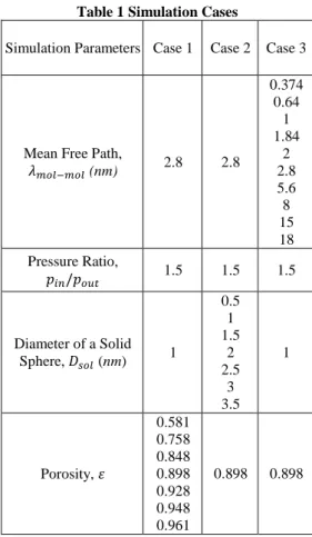
Simulation setups for three cases investigated in this study are given in Table 1. Working fluid is Argon in all cases and its monoatomic diameter is 0.365 nm. The channel dimension is 200×40×40 nm for case 1 and case 2. For case 3, length of the z axis varies from 5 to 200 nm. For the flow properties affected by the cross-sectional area, calculation area of the yz plane is adjusted so that the computational volume does not change
.
The length of the porous medium in the flow direction 𝐿𝑝𝑚 is constant 160 nm in all cases for the accuracy of the comparison. The setup temperature of inside of channel and its boundaries is 300 K. Here, the mean free path calculated by kinetic theory when starting the simulation is in first row, the ratio of pressures of inlet and outlet boundaries of the channel is in second row, diameters of the solid spheres forming the porous medium in third row, and porosity of the porous medium calculated at the beginning of the simulation is given in fourth row.Table 1 Simulation Cases
Simulation Parameters Case 1 Case 2 Case 3
Mean Free Path,
𝜆𝑚𝑜𝑙−𝑚𝑜𝑙 (nm) 2.8 2.8 0.374 0.64 1 1.84 2 2.8 5.6 8 15 18 Pressure Ratio, 𝑝𝑖𝑛/𝑝𝑜𝑢𝑡 1.5 1.5 1.5 Diameter of a Solid Sphere, 𝐷𝑠𝑜𝑙 (nm) 1 0.5 1 1.5 2 2.5 3 3.5 1 Porosity, 𝜀 0.581 0.758 0.848 0.898 0.928 0.948 0.961 0.898 0.898
Reference Cases: 2.8, 1.5, 1, 0.898. There are cases where all three parameters of this reference case are changed separately, but no binary-to-triple changes. Kn increases with decreasing number density. Especially in Kn change in Case 3, the number of molecules must be increased for the EDMD simulation to work more efficiently. Time-based comparisons of the two selected properties in the same flow and simulation conditions but with
different number of simulated molecules were performed in Fig. 2. Accordingly, it was obtained that different z-axis size and the number of molecules associated with it did not change the EDMD results. In fact, the change in size on the z axis does not change the result of tortuosity and permeability, but it affects the mass flow rate as the cross-sectional area of the channel changes. This situation was taken into consideration and the calculation cross-section area was kept constant for all cases.
Simulation time shown in Fig. 2(a) and (c) is the real time of simulation and is the sum of the interval time of occurrence of each event during the simulation. Wall clock time shown in Fig. 2(b) and (d) is the elapsed time of the computer. The simulation with higher number of molecules has no effect on the steady-state values of the properties.
Considering both wall clock and simulation time, both properties converge the same value. Unlike the mesh dependence of results in CFD simulations, EDMD results are independent of number of simulated molecules. The number of molecules provides convenience for data reduction in EDMD. For these reasons, it was found effective to work with 195000 simulated molecules for all cases.
At the beginning of the flow simulation, spherical particles of same diameter were placed in the middle of the channel by cubic alignment. Distance between the particles is calculated according to the desired porosity value and their positions are fixed. At the first moment of the simulation, specular reflection boundary condition was applied to all walls of the channel. The initial velocities of the molecules from the Boltzmann distribution according to the temperature at the first time were initialized to give sufficient collision for thermal homogeneity of molecules distributed to the channel. Then, gas flow simulation in porous media was performed by applying periodic and pressure driven flow boundary conditions.
Increasing diameters of the solid spheres by keeping the porosity constant requires proportionally increasing center-to-center distance between the spheres. This also means an increase in pore size. By keeping diameters of the spheres constant, it is sufficient to change the distance between the spheres to change porosity. This also allows us to change pore size while changing porosity. The permeability obtained from the simulation was considered intrinsic permeability under Kn ≪ 1 condition where permeability remained constant for a given porous structure and was used for normalization. In all simulations, for the flow caused by pressure difference at the initial time, only inlet pressure 𝑝𝑖𝑛 was increased and outlet pressure 𝑝𝑜𝑢𝑡was set to the same value as the in-channel pressure. In order to create a pressure gradient, the inlet pressure was set to a multiple of the channel pressure, i.e. pressure ratio 𝑝𝑖𝑛/𝑝𝑜𝑢𝑡 was setup. The inlet and outlet pressures and pressure in the medium spontaneously occurred during the simulation. In order to avoid characteristic length confusion, 𝜆𝑚𝑜𝑙−𝑚𝑜𝑙 was given instead of Kn as rarefaction parameter of the flow in
the setup of the simulation. It is calculated with Eq. (1). However, Kn in the pore during the simulation
was calculated by Eq. ().
Fig. 2. (a) and (b) Normalized Tortuosity vs. Simulation and Wall Clock Time, (c) and (d) Normalized Permeability vs. Simulation and
Wall Clock Time.
Fig. 3. ε vs. (a) Mass flow rate, (b) µe, (c) τ and
(d) K/Dsol2 for Case 1.
0 0.2 0.4 0.6 0.8 1 1.2 1.4 0 0.2 0.4 0.6 0.8 1 No rm a li ze d To rtu o sity
Normalized Simulation Time
Nm=100000 Nm=150000 Nm=200000
(a)
0 0.2 0.4 0.6 0.8 1 1.2 1.4 0 0.2 0.4 0.6 0.8 1 No rm a li ze d To rtu o sityNormalized Wall Clock Time
Nm=100000 Nm=150000 Nm=200000
(b)
0 0.1 0.2 0.3 0.4 0.5 0.6 0.7 0.8 0.9 1 0 0.2 0.4 0.6 0.8 1 No rm a li ze d Per m ea b il it yNormalized Simulation Time
Nm=100000 Nm=150000 Nm=200000
(c)
0 0.1 0.2 0.3 0.4 0.5 0.6 0.7 0.8 0.9 1 0 0.2 0.4 0.6 0.8 1 No rm a li ze d Per m ea b il it yNormalized Wall Clock Time
Nm=100000 Nm=150000 Nm=200000
(d)
0 2 4 6 8 10 12 14 16 18 0.5 0.6 0.7 0.8 0.9 1 0 20 40 60 80 100 120 140 160 180 M a ss Flo w Ra te /1 0 12(k g /s) ε Flo w Ve lo cit y(m /s) Flow Velocity Mass Flow RateCase 1
(a)
1 2 3 4 5 0.5 0.6 0.7 0.8 0.9 1 𝜇e (Pa .s)/1 0 5 ε Case 1(b)
1 10 100 0 0.2 0.4 0.6 0.8 1 τ εBruggeman, (1935), α=2.5, continuum regime Comiti et al. (1989), P=0.63, continuum regime Pisani (2011),flat parallelepiped,continuum regime Tomadakis et al., (1993), continuum regime Tomadakis et al., (1993), transition regime
Case 1
(c)
0 0.2 0.4 0.6 0.8 1 1.2 1.4 1.6 0 0.2 0.4 0.6 0.8 1 K/D sol 2 εYu et al., (2002), continuum regime Chen et al., (2017), continuum regime G.Yang et al., (2018), continuum regime Mostafavi et al., (2017), transition regime Shariati et al., (2019), Dsol=1000nm, transition regime EDMD, transition regime
Case 1
5. RESULTS AND DISCUSSIONS
The effects of porosity, sphere diameter and Kn on the basic parameters such as flow velocity, mass flow rate, viscosity, tortuosity and permeability are investigated in Fig. 3 and 4.
Kn obtained from molecule-solid sphere and molecule-molecule collision frequency ratio in the porous medium and the ratio of the mean free path to distance between the centers of two spheres for mol-mol collision are quite approximate. The calculated 𝛼𝑠𝑖𝑚 coefficient is approximately 1.6.
If one changes only porosity in the setup by keeping mean free path, solid sphere diameter, and pressure gradient constant, flow velocity and mass flow rate change in the porous medium as in Fig. 3(a). As resistance to flow decreases with increasing porosity, the velocity and flow rate of the molecules in the flow direction increases. This increase rate reaches the largest value as porosity approaches 1.
In Case 1 conditions, viscosity in the porous medium is found to be nearly independent from porosity (Fig. 3(b)).
As porosity increases, the collision frequency of molecule with solid sphere will decrease and this decreases viscosity of the gas a little bit.
The relationship between tortuosity and porosity obtained in the EDMD study was compared with some experimental model and simulation results in the literature for same flow conditions in Fig. 3(c). Porosity has a value of 1 in continuum flow regime while tortuosity has a value greater than 1 in the transition regime. At porosity greater than 0.8, EDMD simulation seems to be consistent with the literature, but it is common for all literature comparisons to see different results at low porosity. But nano-sized particles cause greater tortuosity than macro-sized particles in the same porosity change. If only porosity is changed for a fixed sphere diameter, permeability of the porous medium changes. That was experienced by EDMD simulation and compared with some models in Fig. 3(d). Accordingly, the increase in porosity leads to an increase in permeability. It is obvious that the porosity value of 0.4 and above especially affects the permeability a lot. Here the properties of the porous structure put different results for different studies. The results in the transition regime were larger than in the continuous regime for values greater than 0.4. Fig. 4(a) shows the effect of sphere diameter on flow velocity and flow rate for constant porosity. At 2.5 nm below the sphere diameter, the rate of increase in flow velocity and flow rate is higher than in the values above. The two flow characteristics do not change significantly after this critical diameter. In Fig. 4(b), viscosity changes in the porous medium versus the sphere diameter are given. While the diameter is close to diameter of the fluid gas particle, the viscosity is quite high, but as this diameter gets larger, viscosity decreases as the momentum transfer with the solid sphere decreases.
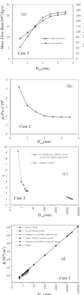
Fig. 4. Dsol vs. (a) Mass flow rate, (b) µe, (c) τ and
(d) K for Case 2. 0 20 40 60 80 100 120 140 160 180 200 0 5 10 15 20 25 0 1 2 3 4 Fl o w Velo cit y(m /s) M a ss Flo w Ra te /1 0 15(kg /s) Dsol(nm)
Mass Flow Rate Flow Velocity Case 2
(a)
0 1 2 3 4 5 6 0 1 2 3 4 𝜇e (Pa .s)/1 0 5 Dsol(nm) Case 2(b)
0 1 2 3 4 5 6 7 8 9 10 0 .1 1 10 1 0 0 1 0 0 0 1 0 0 0 0 1 0 0 0 0 0 τ Dsol(nm) R. Vallabh et al. (2010), 𝜀=0.85, continuum regime, experiment EDMD, 𝜀=0.898 Case 2(c)
0 .1 1 10 1 00 1 0 0 0 1 0 0 0 0 1 0 0 0 0 0 K /1 0 20 (m 2) Dsol(nm) Ergun, (1952) Yu and Cheng, (2002) Koponen et al.(1998), experimental Davies (1952), empirical model Koponen et al.(1997), empirical model EDMD Case 2 1012 -1011 -1010 -109 -108 -107 -106-(d
Fig. 5. Kn vs. (a) Nondimensional mass flow rate, (b) µe/µ0, (c) τ and (d) K/Kint for Case 3.
This drop decreases as the diameter grows and becomes almost invariable. In the Dsol values where Kn is in the transition regime, slip flow effects become dominant and tortuosity tends to increase rapidly. Thus, as can be seen from Fig. 4(c), the larger tortuosity from EDMD results can be due to the solid sphere dimensions that form the porous medium. Diameters of the solid particles in other experimental models are in μm or mm, while in our study it is in nm. If we keep porosity of the porous medium constant and increase diameter of the solid spheres, permeability increases as in Fig. 4(d). Ratio of diameter of the solid spheres to diameter of the flowing gas molecules is effective in this increase. EDMD and other models seem to become more compatible as 𝐷𝑠𝑜𝑙 approaches 0.5 nm. However, it was revealed that for the same sphere diameter transition regime caused lower permeability than the continuous regime.
In Fig. 5(a), the dependence of mass flow rate on Kn is compared with different studies. The increase of Kn increases the number of individual collisions of molecules with solid spheres. As a result, the viscosity initially increases, which in turn reduces mass flow rate. Then increase in Kn increases velocity slip, which leads to an increase in mass flow rate. In this study, lowest mass flow rate, known as Kn minimum (Knudsen 1909) was obtained at Kn≈0.94. What makes this value below 1 is an effect of porous media and tortuosity. The EDMD result in the graph is normalized to this value.
The relationship between gas viscosity and Kn in the transition regime is shown in Fig. 5(b). The relationship we obtained from EDMD simulation was compared with some models. Viscosity is highly dependent on Kn in the transition regime. Viscosity tends to decrease with increasing slip effects and Kn. In this study, although the collision of the molecule with the solid was made according to the specular reflection model, Michalis et al. (2010) argued that the dependence of viscosity on Kn in the transition regime was similar for other reflection models. The path of the molecules flowing in a narrower pore size gets longer. It was discovered that it is different from the normal wall channel only in the transition regime but similar for other regimes.
Fig. 5(c) shows how tortuosity depends on Kn. The porous structure difference caused the deviation of porosity-related tortuosity values, although partially consistent. However, effect of the transition regime on tortuosity is clearly demonstrated in the EDMD simulation. Although it is not shown in this study, the increase in Kn together with increasing porosity effect of tortuosity less than in the study of Zalc et al (2004) stated. In transition flow, viscous flow rules lose their validity, so it is impossible to use the basic Darcy model to validate EDMD results. We have to take advantage of permeability models based on Kn. The porosity of 0.8, consisting of fiber structures, and the porosity of about 0.9 made from spheres modeled in this study are the same. This relationship, which has not been adequately studied in the literature, was confirmed by this study.
Effect of Kn is clearly shown in Fig. 5(d). In 0 1 2 3 4 5 6 7 8 9 10 11 12 13 0.01 0.1 1 10 100 No n d im . M a ss Flo w Ra te Kn Cercignani et al., (2004) LBM, Guo and Zheng, (2008) N-S, Hadjiconstantinou, (2003) Korteweg method, (1878) Bi-Velocity method, (2010) Dadzie & Brenner, (2012) Dongari et al., (2009) A. Beskok, (2010), AR=4 EDMD Case 3
(a)
0 0.2 0.4 0.6 0.8 1 1.2 0.01 0.1 1 10 100 𝜇e / 𝜇0 KnBeskok and Karniadakis (1999), a=1.5 Guo et al.,(2006) Sutherland (1905), a=2 EDMD Case 3
(b)
0 1 2 3 4 5 6 7 0.001 0.01 0.1 1 10 100 τ Kn EDMD, ɛ=0.898Tomadakis & Sotirchos (1993), ɛ=0.8
Case
(c)
0 10 20 30 40 50 60 70 80 90 100 0.001 0.01 0.1 1 10 K/K in t KnBeskok and Karniadakis, (1999) Florence et al., (2007), c=1 Kawagoe et al.,(2016) Ho et al.,(2019) Shariati et al.,(2019) G.Yang and B.Weigand, (2018) EDMD
Case 3
continuum flow regime, change in Kn does not affect permeability. The effect of Kn on permeability does not depend on the structure of the porous medium. In slip flow regime, the permeability is linearly dependent on the Kn and increases slightly. The transition regime where Kn is between 0.1<Kn<10 is the region where permeability varies most. Increase in Kn in this region decreases the friction resistance on the solid surface with increasing slip effects, thus causing permeability to increase rapidly. Permeability does not remain constant as in the Darcy flow. This increase is only result of the rarefaction effect and is independent of porous structure and porosity. These results were also advocated in Klinkenberg's theory. Both the mathematical models and simulations in the transition regime gave specific results for permeability. The difference of this study is that the rapid rise of permeability is at later Kn values.As we increase Kn towards molecular flow regime, we observe that the slope develops more linearly.
6. CONCLUSIONS
By means of EDMD simulation, monoatomic Argon gas flow was performed in a porous medium consisting of solid spheres with the help of pressure boundary condition.
Permeability, viscosity, tortuosity and mass flow rate properties in porous media were evaluated and obtained by EDMD perspective.
New findings which are missing in the literature are presented below.
For the first time in the literature, viscosity was investigated in the porous medium depending on Kn, Dsol and porosity.
This study revealed that the transition regime affects the flow characteristics more than other Kn-related flow regimes. The effects of porosity and particle size forming porous media on mass flow rate, viscosity and tortuosity investigated especially for nano-sized channels.
It has been demonstrated that porosity affects permeability in the same trend regardless of the Kn-related regime but the results in the transition regime were larger than in the continuous regime for values greater than 0.4.
The permeability of the porous medium, tortuosity, dynamic viscosity of the gas interacting with the solid surface, and mass flow rate were calculated for the dependence of Knudsen number (Kn), which is rarefaction parameter, porosity and solid sphere diameter. The effect of porosity on mass flow rate and flow velocity in a porous medium consisting of nanoparticles has been clearly demonstrated. It was found that porosity was directly proportional to the mass flow rate and has little effect on the viscosity of the gas.
While the solid sphere diameter is directly proportional to the mass flow rate, it is reciprocally proportional to the viscosity. However, as the diameter increases above the critical value, this
dependence disappears and becomes independence. The viscosity is constant in continuum flow regime and depends only on gas itself and temperature. However, as shown in this study, with increasing Kn, viscosity decreases significantly, especially in transition regime flow. Mass flow rate decreases up to critical Kn and tends to increase due to slip effect on the solid surface after a value of around 1. It was demonstrated by this study that Knudsen minimum seen in normal channels is also valid for porous media. However, due to effect of tortuosity, Knudsen minimum was observed at a value below 1. In addition, when Kn is 1 and higher, mass flow rate of the porous medium is lower than the normal channel.
The tortuosity of porous media consisting of macro-sized particles has been obtained between 1 and 2 in many experimental and numerical studies.However, the finding that as size of the diameter approaches size of the fluid molecule, tortuosity increases near vertical was obtained from this study.
Tortuosity is reciprocally proportional to solid sphere diameter and porosity, while it is directly proportional to Kn in transition regime. This study shows that as the particle diameter increases for constant porosity, tortuosity decreases and mass flow rate increases. Although porosity is not too low, the decrease in tortuosity decreases for values greater than 2.5 of 𝐷𝑠𝑜𝑙. Unlike continuum flow regime, in transition regime, when porosity is 1, tortuosity is greater than 1.
Permeability is directly proportional to Kn, porosity and diameter of solid sphere. In particular, permeability of the porous medium, which is constant in continuum flow regime, shows a significant increase with the increase in Kn in transition regime.
It was found that the solid sphere diameter in constant porosity is directly proportional to the permeability. Even the comparison with many other methods supported the fact that this direct proportion valids for 1 nm to 100 microns in diameter. In addition, it is verified that tortuosity and permeability do not change depending on the number of molecules flowing in porous media.
REFERENCES
Akkaya, V. R. and I. Kandemir (2015). Event-driven molecular dynamics simulation of hard-sphere gas flows in microchannels.
Mathematical Problems in Engineering, 1–
12.
Alder, B. J. and T. E. Wainwright (1957). Phase Transition for a Hard Sphere System. The
Journal of Chemical Physics 27(5), 1208–
1209.
Bannerman, M. N., Sargant, R. and L. Lue (2011). DynamO: A free O(N) general event-driven molecular dynamics simulator. Journal of
3338.
Beskok, A. and G. E. Karniadakis (1999). Report: A model for flows in channels, pipes, and ducts at micro and nano scales. Microscale
Thermophysical Engineering 3(1), 43–77.
Bird, G. A. (1994). Molecular Gas Dynamics and the
Direct Simulation of Gas Flows. Clarendon
Press, Oxford.
Bruggeman, D. A. G. (1935). Berechnung verschiedener physikalischer Konstanten von heterogenen Substanzen. I. Dielektrizitätskonstanten und Leitfähigkeiten der Mischkörper aus isotropen Substanzen.
Annalen der Physik 416(7), 636–664.
Carman, P. C. (1997). Fluid flow through granular beds. Chemical Engineering Research and
Design 75, S32–S48.
Cercignani, C., M. Lampis and S. Lorenzani (2004). Variational approach to gas flows in microchannels. Physics of Fluids 16(9), 3426–3437.
Chen, X. and G. Yao (2017). An improved model for permeability estimation in low permeable porous media based on fractal geometry and modified Hagen-Poiseuille flow. Fuel,
Elsevier Ltd 210, 748–757.
Comiti, J. and M. Renaud (1989). A new model for determining mean structure parameters of fixed beds from pressure drop measurements: application to beds packed with parallelepipedal particles. Chemical Engineering Science 44(7), pp.1539–1545.
Dadzie, S. K. and H. Brenner (2012). Predicting enhanced mass flow rates in gas microchannels using nonkinetic models. Physical Review E - Statistical, Nonlinear,
and Soft Matter Physics 86(3), 036318.
Danielewski, M. and B. Wierzba (2010). Thermodynamically consistent bi-velocity mass transport phenomenology. Acta Materialia 58(20), 6717–6727.
Darcy, H. (1856). Les fontaines publiques de la ville de Dijon. Recherche.
Davies, C. N. (1952). The Separation of Airborne Dust and Particles. Preedings of Institute of
Mechanical Engineers, Preedings of Institute
of Mechanical Engineers, London.
Donev, A., A. L. Garcia and B. J. Alder (2008). Stochastic Event-Driven Molecular Dynamics. Journal of Computational Physics 227(4), 2644–2665.
Dongari, N., A. Sharma and F. Durst (2009). Pressure-driven diffusive gas flows in micro-channels: From the Knudsen to the continuum regimes. Microfluidics and Nanofluidics 6(5), 679–692.
Ergun, S. (1952). Fluid flow through packed columns. Chemical Engineering Progress 48,
89–94.
Ezzatabadipour, M. and H. Zahedi (2018). Simulation of a fluid flow and investigation of a permeability-porosity relationship in porous media with random circular obstacles using the curved boundary lattice Boltzmann method. The European Physical Journal Plus 133(11), 464.
Florence, F. A. et al. (2007). Improved permeability prediction relations for low-permeability sands. In Society of Petroleum Engineers -
Rocky Mountain Oil and Gas Technology Symposium. 290–307.
Garcia, A. L. and W. Wagner (2006). Generation of the Maxwellian inflow distribution. Journal
of Computational Physics 217(2), 693–708.
Greber, I., C. Sleeter and I. Kandemir (2001). Molecular dynamics simulation of unsteady diffusion. AIP Conference Proceedings,
American Institute of Physics Inc. 396–400.
Guo, Z., T. S. Zhao and Y. Shi (2006). Physical symmetry, spatial accuracy, and relaxation time of the lattice Boltzmann equation for microgas flows. Journal of Applied Physics 99(7).
Guo, Z., C. Zheng and B. Shi (2008). Lattice Boltzmann equation with multiple effective relaxation times for gaseous microscale flow. Physical Review E - Statistical, Nonlinear, and Soft Matter Physics 77(3), 036707. Hadjiconstantinou, N. G. (2003). Comment on
Cercignani’s second-order slip coefficient.
Physics of Fluids 15(8), 2352–2354.
Ho, M. T. et al. (2019). Pore-scale simulations of rarefied gas flows in ultra-tight porous media.
Fuel 249, 341–351.
Jeong, N., D. H. Choi and C. L. Lin (2006). Prediction of Darcy-Forchheimer drag for micro-porous structures of complex geometry using the lattice Boltzmann method. Journal
of Micromechanics and Microengineering
16(10), 2240–2250.
Kalarakis, A. N., V. K. Michalis, E. D. Skouras and V. N. Burganos (2012). Mesoscopic Simulation of Rarefied Flow in Narrow Channels and Porous Media. Transport in
Porous Media 94(1), 385–398.
Kandemir, I. (1999). A multicell molecular dynamics
method [Ph.D. thesis]. Case Western Reserve
University, Cleveland, Ohio, USA.
Kaviany, M. (1966). Principle of Heat Transfer in Porous Media. The British Journal of
Psychiatry 112(483), 211–212.
Kawagoe, Y. et al. (2016). A study on pressure-driven gas transport in porous media: from nanoscale to microscale. Microfluidics and Nanofluidics 20(12), p.162.
porous media to liquids and gases. Drilling
and Production Practice 1941, 200–213.
Knudsen, M. (1909). Die Gesetze der Molekularströmung und der inneren Reibungsströmung der Gase durch Röhren.
Annalen der Physik 333(1), 75–130.
Koponen, A. et al. (1998). Permeability of Three-Dimensional Random Fiber Webs. Physical
Review Letters 80(4), 716–719.
Kozeny, J. (1927). Uber Kapillare Leitung des Wassers im Boden Stizungsberichte. Royal
Academy of Science, Vienna, Proc. Class I,
136, 271–306.
Liou, W. W. and Y. C. Fang (2000). Implicit boundary conditions for direct simulation Monte Carlo method in MEMS flow predictions. CMES - Computer Modeling in
Engineering and Sciences 1(4), 119-128.
Marín, M. and P. Cordero (1995). An empirical assessment of priority queues in event-driven molecular dynamics simulation. Computer
Physics Communications 92(2–3), 214–224.
Michalis, V. K., A. N. Kalarakis, E. D. Skouras and V. N. Burganos (2010). Rarefaction effects on gas viscosity in the Knudsen transition regime. Microfluidics and Nanofluidics 9(4– 5), 847–853.
Mostafavi, M. and A. H. Meghdadi Isfahani (2017). A new formulation for prediction of permeability of nano porous structures using lattice botzmann method. Journal of Applied
Fluid Mechanics10(2), 639–649.
Paul, G. (2007). A Complexity O(1) priority queue for event driven molecular dynamics simulations. Journal of Computational Physics 221(2), 615–625.
Pisani, L. (2011). Simple Expression for the Tortuosity of Porous Media. Transport in
Porous Media 88(2), 193–203.
Rapaport, D.C. (1980). The event scheduling problem in molecular dynamic simulation. Journal of Computational Physics 34(2), 184– 201.
Shariati, V., Ahmadian, M. H. and Roohi, E. (2019). Direct Simulation Monte Carlo investigation of fluid characteristics and gas transport in porous microchannels. Scientific Reports
9(1), 17183.
Sutherland, W. (1905). LXXV. A dynamical theory of diffusion for non-electrolytes and the molecular mass of albumin . The London,
Edinburgh, and Dublin Philosophical Magazine and Journal of Science 9(54), 781–
785.
Tjaden, B., D. J. L. Brett and P. R. Shearing (2018). Tortuosity in electrochemical devices: a review of calculation approaches.
International Materials Reviews 63(2), 47–
67.
Tomadakis, M. M. and T. J. Robertson (2005). Viscous permeability of random fiber structures: Comparison of electrical and diffusional estimates with experimental and analytical results. Journal of Composite
Materials 39(2), 163–188.
Tomadakis, M. M. and S. V. Sotirchos (1993). Ordinary, transition, and Knudsen regime diffusion in random capillary structures.
Chemical Engineering Science 48(19), 3323–
3333.
Vallabh, R., P. Banks-Lee and A. F. Seyam (2010). New approach for determining tortuosity in fibrous Porous Media. Journal of Engineered
Fibers and Fabrics 5(3), 7–15.
Wu, J. and B. Yu (2007). A fractal resistance model for flow through porous media. International
Journal of Heat and Mass Transfer 50(19–
20), 3925–3932.
Yang, G. and B. Weigand (2018). Investigation of the Klinkenberg effect in a micro/nanoporous medium by direct simulation Monte Carlo method. Physical Review Fluids, American
Physical Society 3(4).
Yu, B. and P. Cheng (2002). A fractal permeability model for bi-dispersed porous media.
International Journal of Heat and Mass Transfer 45(14), 2983–2993.
Zalc, J. M., S. C. Reyes and E. Iglesia (2004). The effects of diffusion mechanism and void structure on transport rates and tortuosity factors in complex porous structures.
Chemical Engineering Science 59(14), 2947–