T.C.
SELÇUK ÜNİVERSİTESİ FEN BİLİMLERİ ENSTİTÜSÜ
LIU TYPE LOGISTIC ESTIMATORS Yasin ASAR
DOKTORA TEZİ İstatistik Anabilim Dalı
Ocak-2015 KONYA Her Hakkı Saklıdır
iv ÖZET DOKTORA TEZİ
LİU TİPİ LOJİSTİK REGRESYON TAHMİN EDİCİLERİ Yasin ASAR
Selçuk Üniversitesi Fen Bilimleri Enstitüsü İstatistik Anabilim Dalı
Danışman: Prof.Dr. Aşır GENÇ 2015, 99 Sayfa
Jüri
Prof. Dr. Aşır GENÇ Doç. Dr. Coşkun KUŞ Doç. Dr. Murat ERİŞOĞLU
Doç. Dr. İsmail KINACI Yrd. Doç. Dr. Aydın KARAKOCA
Binari lojistik regresyon modellerinde çoklu bağlantı problemi en çok olabilirlik tahmin edicisinin varyansını şişirmekte ve tahmin edicinin performansını düşürmektedir. Bu nedenle doğrusal modellerde çoklu bağlantı problemini gidermek için önerilen tahmin ediciler lojistik regresyona genelleştirilmiştir. Bu tezde, bazı yanlı tahmin edicilerin lojistik versiyonları gözden geçirilmiştir. Ayrıca, yeni bir genelleştirme yapılarak daha öncekilerle MSE kriteri bakımından performansı karşılaştırılmıştır. Yeni önerilen tahmin edici iki parametreli olduğundan parametrelerin seçimi için tekrarlı (iterative) bir metot önerilmiştir.
Anahtar Kelimeler: Binari lojistik regresyon, çoklu bağlantı, hata kareler ortalaması, Monte Carlo simülasyonu, MSE, yanlı tahmin edici.
v ABSTRACT
Ph.D THESIS
LIU TYPE LOGISTIC ESTIMATORS
Yasin ASAR
THE GRADUATE SCHOOL OF NATURAL AND APPLIED SCIENCE OF SELÇUK UNIVERSITY
THE DEGREE OF DOCTOR OF PHILOSOPHY IN STATISTICS
Advisor: Prof.Dr. Aşır GENÇ 2015, 99 Pages
Jury
Prof. Dr. Aşır GENÇ Assoc. Prof. Dr. Coşkun KUŞ Assoc. Prof. Dr. Murat ERİŞOĞLU
Assoc. Prof. Dr. İsmail KINACI Asst. Prof. Dr. Aydın KARAKOCA
Multicollinearity problem inflates the variance of maximum likelihood estimator and affects the performance of this estimator negatively in binary logistic regression. Thus, biased estimators used to overcome this problem have been generated to logistic regression. Some of these estimators are reviewed in this thesis. Moreover, a new generalization is proposed to overcome multicollinearity performances of estimators are compared in the sense of MSE criterion. Since new estimator has two parameters, an iterative method is proposed to choose these parameters.
Keywords: Biased estimator, binary logistic regression, mean squared error, Monte Carlo simulation, MSE, multicollinearity
vi PREFACE
First and foremost I want to thank my advisor Prof. Dr. Aşır Genç for his support and guidance, for his patience and kindness. It has been an honor to be his Ph.D. student. I appreciate all his contributions to make my Ph.D. experience productive and stimulating, He has been very inspring for me.
I would also like to thank my committee members Assoc. Prof. Dr. Coşkun Kuş and Assist. Prof. Dr. Aydın Karakoca for their guidance.
I am also grateful to Assoc. Prof. Dr. Murat Erişoğlu, as he was always there to help. His guidance and helpful contributions make the thesis more comprehensive. I also appreciate his theoretical contributions to the thesis.
Lastly and most importantly, I would like to express immense appreciation and love to my wife and daughter. Without them, I simply would not be here. I owe them my success. Thank you for being so patient and kind.
Yasin ASAR KONYA-2015
vii CONTENTS ÖZET ... iv ABSTRACT ... v PREFACE ... vi CONTENTS ... vii
SYMBOLS AND ABBREVIATIONS ... ix
1. INTRODUCTION ... 1
1.1. Review of the Literature ... 5
2. MULTICOLLINEARITY... 8
2.1. Definition of Multicollinearity ... 8
2.1.1. A graphical representation of the problem ... 8
2.2. Sources of Multicollinearity ... 11
2.3. Consequences of Multicollinearity ... 11
2.4. Multicollinearity Diagnostics ... 12
2.5. Some Methods to Overcome Multicollinearity ... 14
3. BIASED ESTIMATORS IN LINEAR MODEL ... 15
3.1. Ridge Estimator ... 16
3.1.1. MSE properties of ridge estimator ... 17
3.1.2. Selection of the parameter k ... 19
3.1.3. New proposed ridge estimators ... 25
3.1.4. Comparison of the ridge estimators: A Monte Carlo simulation study .... 26
3.1.5. Some conclusive remarks regarding ridge regression and simulation ... 32
3.2. Liu Estimator ... 36
3.3. Liu Type Estimator ... 37
3.4. Another Two Parameter Liu Type Estimator ... 38
3.5. Two Parameter Ridge Estimator ... 40
4. BIASED ESTIMATORS IN LOGISTIC MODEL: NEW METHODS ... 44
4.1. Logistic Ridge Estimator ... 46
4.1.1. MMSE comparison of MLE and LRE ... 48
4.2. Logistic Liu Estimator ... 49
4.2.1. MMSE comparison of MLE and LLE ... 51
4.3. Logistic Liu-Type Estimator ... 52
4.3.1. MMSE and MSE comparisons of MLE and LT1 ... 54
4.3.2. A Monte Carlo simulation study ... 55
4.3.3. Results and discussions regarding the simulation study ... 57
4.3.4. Summary and conclusion ... 60
viii
4.4.1. MMSE and MSE comparisons of MLE and LT2 ... 61
4.4.2. Proposed estimators of the shrinkage parameter d ... 62
4.4.3. A Monte Carlo simulation study ... 63
4.4.4. The results of the Monte Carlo simulation ... 64
4.4.5. An application of real data ... 66
4.4.6. Summary and conclusion ... 67
5. A NEW BIASED ESTIMATOR FOR THE LOGISTIC MODEL ... 68
5.1. MMSE Comparisons Between The Estimators ... 69
5.1.1. The Comparison of MLE and YA ... 69
5.1.2. The Comparison of LRE and YA ... 70
5.1.3. The Comparison of LLE and YA ... 70
5.1.4. The Comparison of LT1 and YA ... 71
5.1.5. The Comparison of LT2 and YA ... 72
5.2. Selection Processes of the Parameters d k, and q... 72
5.3. Design of the Monte Carlo Simulation Study ... 75
5.4. Results of the Simulation and Discussions ... 76
5.5. Real Data Application 1 ... 78
5.6. Real Data Application 2 ... 86
5.7. Some Conclusive Remarks ... 91
6. CONCLUSION AND SUGGESTIONS ... 92
6.1. Conclusion... 92
6.2. Suggestions ... 93
7. REFERENCES ... 94
ix SYMBOLS AND ABBREVIATIONS
Symbols
Bias : Bias of the vector
diag X : Diagonal of the matrix X
E : Expected value of the random variable
Var : Variance-covariance matrix of the random variable
Cov X Y , : Covariance of the random variables X and Y
rank X : Rank of the matrix X
tr X : Trace of the matrix X
ab : Vector a is orthogonal to vector b 2
: Variance of the error terms in linear regression model n
I : n n identity matrix
2
~N 0, In
: Vector is distributed norrmally with zero mean and variance 2
n I
i j
X x : Another representation of the matrix X such that xi j is the element placed in ith row and j column of the matrix X th
X : Determinant of the matrix X
1X : Inverse of the matrix X
X : Transpose of the matrix X : Euclidean norm of the vector
x Abbreviations
p.d. : positive definite
IWLS : Iteratively weighted least squares LLE : Logistic Liu estimator
LRE : Logistic ridge estimator LT1 : Liu-type logistic estimator
LT2 : Another Liu-type logistic estimator
MAE : Mean absolute error
MLE : Maximum likelihood estimator MMSE : Matrix mean square error
MSE : Mean square error
OLS : Ordinary least squares VIF : Variance Inflation Factors
1. INTRODUCTION
Regression analysis is one of the most widely used statistical techniques which can be applied to investigate and model the relationship between variables. There is a wide range of applications of regression such as engineering, the physical and chemical sciences, economics, management and the social sciences (Montgomery et al., 2001).
Multiple linear regression is used to predict the values of a dependent variable when there are more than one explanatory variables (regressor). A multiple linear regression model can be expressed as follows:
Y X (1.1)
where Y is an n1 vector of dependent variable, X is an np data matrix (design matrix) whose columns are the explanatory variables, is a p1 vector of unknown regression coefficients and is an n1 vector of random errors following the normal distribution with zero mean and variance 2 i.e., ~N
0,2I
where I is an n n identity matrix.There are some assumptions on the random error term in multiple linear regression models as follows:
1. The error terms i, i1, 2,...,n are independent of each other and random, 2. E
i 0, i1, 2,...,n3. Var
i 2, Var is the variance function, i1, 2,...,n4. Cov
i, j
0, Cov is the covariance function, i j,1 i j n5. Xj, X is the j j column vector of the matrix X such that th
1, 2,...,
j p and X X X1, 2,...,Xp,
6. The elements of the matrix X are constants and it has full rank, i.e.,
rank X p,
7. The matrix X X is non-singular,
8. ~N
0,2In
is true for the hypothesis tests and the error terms are the random variables following the normal distribution,The above assumptions can be summarized in five basic assumptions (Allison, 1999; Aydın, 2014) namely,
1. Y X means that Y is a linear function of X and a random error term .
2. E
i 0, i1, 2,...,n implies that the error terms have zero mean and more importantly the expected value of does not change with X implying that X and are not correlated.3. Var
i 2, i1, 2,...,n provides that the variance of is the same for all observations, this property is called homoscedasticity.4. Cov
i, j
0, i j,1 i j n means that random errors are independent of each other.5. ~N
0,2In
means that the error terms are distributed normally.On the other hand, logistic regression or logit regression is a type of probabilistic statistical classification model (Bishop, 2006). It is also used for predicting the outcome of a categorical dependent variable. Logistic regression measures the relationships between a categorical dependent variable and one or more independent variables, which are usually (not necessarily) continuous, by using probability scores as the predicted values of a dependent variable (Bhandari and Joensson, 2011).
Logistic regression can be binomial or multinomial. Binomial (binary) logistic regression is a type of regression analysis where the dependent (response) variable is dichotomous and the explanatory (independent) variables are continuous, categorical or both. In logistic regression, there is no assumption that the relationship between the independent variables and the dependent variable is linear, thus it is a nonlinear method being a useful tool in order to analyze data including categorical response variables.
The binary logistic regression model has become the popular method of analysis in the situation that the outcome variable is discrete or dichotomous. Although, its original acceptance is important in the field of epidemiologic researches, this method has become a commonly employed method in the area of applied sciences such as engineering, health policy, biomedical research, business and finance, criminology, ecology, linguistics and biology (Hosmer and Lemeshow, 2000).
It is very important to understand that using logistic regression model for a dichotomous dependent variable as a predictive model is a better approach than using
the ordinary linear regression. It is known that if the five basic assumptions of the linear regression are satisfied, ordinary least squares (OLS) estimates of the regression coefficients are unbiased and have minimum variance. However, if the dependent variable is assumed to be dichotomous, then it can be observed that if the first and second assumptions are true, then third and fifth ones are definitely false.
For example, if the fifth assumption is considered, it is easy to observe that the error terms can only take two values implying that it is not possible for them to have a normal distribution. If the variance of the errors is considered, then first assumption implies that variance of i equals to variance of y . Generally, the variance of a dummy i variable is pi
1pi
where p is the probability that i yi 1. Thus, the following equation holds:
Var i pi 1pi xi 1xi . But this equation says that the variance of i differs for different observations which violates the third assumption. For a great discussion of this situation see Allison (1999), Chapter 2.
Off course, after determining the difference between the logistic regression and the linear regression in terms of the choice of parametric model and the assumptions, one can assess the regression analysis using the same general principles used in the linear regression model (Midi et al., 2010) .
In order to satisfy the validity of the model, it has to satisfy the assumptions of logistic regression. The followings are the general assumptions involves in logistic regression analysis (UCLA, 2007):
1. The conditional probabilities are a logistic function of the explanatory variables,
2. No important variables are omitted, 3. Irrelative variables are not included,
4. The explanatory variables are measured without error, 5. The observations of the variables are independent,
6. There is no linear dependency between the explanatory variables, 7. The errors of the model are distributed binomially.
Both in multiple linear regression models and binary logistic regression models, one may not verify the given assumptions most of the time. The assumptions 5, 6 and 7 of the linear model and the sixth assumption of the logistic model imply that there should be no linear dependency between the explanatory variables or the columns of the
matrix X . In other words, the explanatory variables are said to be orthogonal to each other. However, the regressors are not orthogonal in most of the applications. The multicollinearity (collinearity or ill-conditioning) problem arises when at least one linear function of the explanatory variables is nearly close to zero (Rawlings et al., 1998).
The main point is that, if there is collinearity within the explanatory variables, it is hardly possible to obtain statistically good estimates of their distinct effects on some dependent variable. In the next chapter, the causes, results and the diagnostics of the multicollinearity problem are given in detail.
In this thesis, Maximum likelihood estimator (MLE) and the following methods proposed to overcome multicollinearity are considered: Ridge estimator, Liu estimator, Liu-type estimators and a two-parameter ridge estimator. These estimators are successfully used in linear regression model. However, they have been adapted to the logistic regression model except for the two parameter ridge estimator recently. In this study, the logistic version of the two parameter ridge estimator is defined and the above estimators are compared by using the matrix mean squared error (MMSE) and mean squared error (MSE) criteria in the logistic regression model. Both some theoretical comparisons in the sense of MMSE and numerical comparisons via Monte Carlo simulation studies are given. In the simulations, MSE criterion is used to compare the performances of the estimators.
The purposes of this study are as follows: Some new ridge regression estimators are defined for the linear model in Chapter 3 and these new estimators are used in the logistic versions of the above mentioned estimators successfully in Chapter 4; moreover, some new optimal shrinkage parameters are proposed to use in Liu-type estimators to decrease the variance of the estimator in logistic regression model in Section 4.4; finally, a new two parameter ridge estimator is defined for the logistic regression model and it is showed by conducting an extensive Monte Carlo simulation that this new estimator is better than above estimators in the sense of MSE criterion.
The organization of the thesis is as follows: In Chapter 2, formal definition of multicollinearity, a graphical representation of the problem, sources and consequences of multicollinearity are given. Moreover, multicollinearity diagnostics are reviewed.
In Chapter 3, biased estimators in linear model which can be used to solve collinearity problem are reviewed. The definition of ridge estimator and its MSE
properties are given. Also, some new ridge estimators are defined and their performances are demonstrated via a Monte Carlo simulation study in Section 3.1.
In the remaining parts of Chapter 3, Liu estimator, Liu type estimator, another two parameter Liu type estimator and finally a two parameter ridge estimator are given and some properties of them are reviewed.
In Chapter 4, brief introductory information regarding logistic regression is given. Logistic versions of the mentioned estimators are discussed. In Section 4.1, the logistic ridge estimator is given and MMSE comparison of maximum likelihood estimator and logistic ridge estimator is obtained. In Section 4.2, logistic version of Liu estimator called logistic Liu estimator is discussed and MMSE comparison of MLE and logistic Liu estimator is obtained. In Section 4.3, logistic Liu type estimator is reviewed and MMSE comparison between MLE and this estimator is obtained. Moreover, a Monte Carlo simulation study is designed to compare some existing ridge estimators and the new estimators defined in Chapter 3 in logistic regression. In Section 4.4, another two-parameter Liu-type estimator is given in logistic regression. Again MMSE and MSE comparisons are obtained. Moreover, some new shrinkage estimators are defined to be used in logistic Liu type estimator and a Monte Carlo experiment is conducted to evaluate the performances of these estimators. Finally, an application to real data is demonstrated.
In Chapter 5, a new two parameter logistic ridge estimator is defined. In Section 5.1, MMSE comparisons between the new estimator and the other reviewed estimators are obtained. In Section 5.2, some new iterative selection processes of the parameters are defined. In Section 5.3, a Monte Carlo simulation is designed to compare the performances of all logistic estimators discussed in the thesis. Finally, two real data applications are illustrated.
In the last chapter, a brief summary and conclusion are given and some future suggestions for the practitioners are provided.
1.1. Review of the Literature
There are many distribution functions proposed for using in the analysis of a dichotomous dependent variable, see Cox and Snell (1989). However, the logistic distribution being an extremely flexible and easily used function and providing
clinically meaningful interpretation, it has become the popular distribution in this research area.
The weighted sum of squares can be minimized approximately by using the maximum likelihood estimator. However, this estimator becomes instable when the explanatory variables are intercorrelated. Thus, due to high variance and very low t-ratios, the estimations of MLE are no more trustful. This is because the weighted matrix of cross-products becomes ill-conditioned when there is multicollinearity.
There are some solutions to this problem. One of them is so called ridge regression which is firstly defined by Hoerl and Kennard (1970) for the linear model. Ridge estimator has been adjusted to binary logistic regression model by Schaefer et al. (1984) successfully. The authors applied the ridge estimators defined by Hoerl and Kennard (1970) and Hoerl et al. (1975) in logistic regression.
Recently, Månsson and Shukur (2011) have applied and investigated a number of logistic ridge estimators. By conducting a Monte Carlo experiment, they investigated the performances of MLE and logistic ridge estimators in the presence of multicollinearity under different conditions. According to the results of the simulation, logistic ridge estimators have better performance than MLE.
Kibria et al. (2012) generalized different types of estimation methods of the ridge parameter proposed by Muniz et al. (2012) to be used for logistic ridge regression. They evaluated the performances of the estimators via a Monte Carlo simulation. In the simulation study, they also calculated the average values and the standard deviations of the ridge parameter. Results showed that logistic ridge estimators outperform the MLE approach.
In the study of Månsson et al. (2012), a new shrinkage estimator which is a generalization of the estimator defined by Liu (1993) is proposed. Using MSE, the optimal value of the shrinkage parameter is obtained and some methods of estimation are given. Since logistic Liu estimator uses shrinkage parameter, its length becomes smaller than the length of MLE. The authors showed that logistic Liu estimator has a better performance than MLE according to MSE and mean absolute error (MAE) criteria.
Huang (2012) defined a biased estimator which is a combination of logistic ridge estimator and logistic Liu estimator in order to combat multicollinearity. Necessary and sufficient conditions for the superiority of this estimator over MLE and logistic ridge
estimator are given. Moreover, a Monte Carlo simulation is designed to evaluate the performances of the estimators numerically.
Finally, logistic Liu-type estimator defined by Inan and Erdogan (2013) can also be used a solution to the problem. There are two parameters used in this estimator which seems to be a combination of ridge estimator and Liu estimator. It is showed that logistic Liu-type estimator has a better performance than MLE and logistic ridge estimator defined by Schaefer et al. (1984) in the sense of MSE. Moreover, a real data application is given in the paper.
2. MULTICOLLINEARITY
In the first chapter, informal definition of collinearity which was firstly introduced by Frisch (1934) is given such that the problem occurs when there is a strong linear relation between the explanatory variables. In this chapter, formal definition of multicollinearity, sources and results of it and diagnostics of the problem are discussed.
2.1. Definition of Multicollinearity
It is given that X X X1, 2,...,Xp and Xj contains the n observations of the th
j regressor. Now, the formal definition of multicollinearity can be written in terms of
the linear dependencies of the columns of X . The vectors X X1, 2,...,Xp are linearly dependent if there is a set of constants a a1, 2,...,ap, not all zero, such that
1 0 p j j j a X
. (2.1)If the left hand side of the above equation is equal to zero, it is said that the data set has perfect (or exact) multicollinearity, i.e., the correlation coefficient between the two regressors is 1 or -1. In this case, the rank of the matrix X X becomes less than p and the inverse of it does not exists. However, if equation (2.1) holds for some subset of the columns of X , then there is a near-linear dependency in X X and the problem of collinearity exists. Then the matrix X X is said to be ill-conditioning.
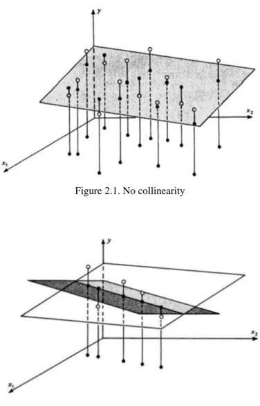
2.1.1. A graphical representation of the problem
The nature of the collinearity problem can be exhibit geometrically with the following figures. The figures are taken from Belsley et al. (2005). Some situations of the model yi 01xi12xi2i,i1, 2,...,n are given. In the figures below, the scatters of the observations are shown. In the x x1, 2”floor” are
x x1, 2
scatters (points denoted by ), while above the data cloud resulting when the y dimension included (points denoted by ) is shown. Figure 2.1 shows the case that x x are not collinear. 1, 2 The well-defined least squares plane is represented by data cloud above. The yintercept of this plane is the estimate of 0 and the partial slopes in the x and 1 x 2
directions are the estimations of 1 and 2 respectively.
Figure 2.1. No collinearity
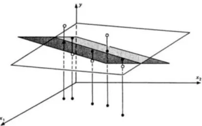
Figure 2.2. Exact collinearity
Figure 2.2 exhibits the case of perfect multicollinearity between x and 1 x . One 2
can see that there is no plane of data cloud i.e., the plane of least squares is not defined. Figure 2.3 shows strong collinearity (but not perfect). The plane of least squares is ill-defined since the least square estimates are imprecise i.e., their variance inflate.
Figure 2.3. Strong collinearity: All coefficients ill-determined
Figure 2.4. Strong collinearity: Constant term well-determined
It is known that multicoliinearity may not inflate all of the parameter estimates. This situation is represented in Figure 2.4 such that the estimates of 1 and 2 are imprecise but the estimate of the intercept term is precise. Similarly, the estimate of 2 is precise however, 0 and 1 have estimates lack of precision as shown in Figure 2.5.
2.2. Sources of Multicollinearity
There are several sources of collinearity. The followings are four primary sources of collinearity (Montgomery et al., 2001):
1. The data collection method employed: When the researcher samples only a subspace of the region of the explanatory variables defined by equation (2.1). 2. Constraints on the model or in the population: When physical constraints are present, multicollinearity exists regardless of the sampling method employed. These constraints generally occur in problems involving production or chemical processes, where the regressors are the components of a product, and these components add to a constant.
3. Model specification: It is possible that adding a polynomial term into a regression model can cause ill-conditioning in the matrix X X .
4. An overdefined model: If a model has more explanatory variables than observations, it is called an overdefined model. According to Gunst and Webster (1975), there are three things to do: First one is to redefine the model in terms of a smaller set of explanatory variables; second is to perform preliminary studies using only subsets of the original explanatory variables; finally using some methods such as principal components analysis to decide which variables to remove from the model.
2.3. Consequences of Multicollinearity
If there is multicollinearity problem with the data set X, one can face the following consequences:
1. The ordinary least squares (OLS) estimator used in linear model or MLE used in logistic model are unbiased estimators of the coefficient vector. They
have large variance and covariance which make the estimation process difficult.
2. The lengths of the unbiased estimators mentioned above tend to be so large in absolute value. It is easy to see this by computing the squared distance between the unbiased estimators and the true parameter. To compute this distance, one should find the diagonal elements of the matrix
X X
1. Since some of the eigenvalues of the matrix X X will be close to zero in the presence of collinearity, the inverse of that eigenvalue becomes too large (may be infinity in worst case). Thus, the squared distance becomes too large.3. Because of the first consequence, the confidence intervals of the coefficients become wider which leads to the acceptance of the null hypothesis.
4. Similarly, t-ratios of the coefficients become statistically insignificant. 5. However, the measure of goodness of fit R may be very high, although the 2
t-ratios are insignificant.
6. The unbiased estimators and their standard errors are very sensitive to small changes in values of the observations.
7. Finally, multicollinearity problem can affect the model selection seriously. The increase in the sample standard errors of coefficients virtually assures a tendency for relevant variables to be discarded incorrectly from regression equations (Farrar and Glauber, 1967).
2.4. Multicollinearity Diagnostics
There are several techniques that can be used for detecting multicollinearity. Some of them which directly determine the degree of collinearity and satisfy information in determining which regressors are involve in collinearity are given as follows:
1. Correlation Matrix: After standardizing the data, the matrix X X becomes the correlation matrix. Let X X ri j such that ri j represents the correlation between the variables x and i xj. The more the linear dependency is, the more |ri j | becomes close to 1. However, this criterion shows only pairwise correlations ,i.e., if more than two
variables are involved in the collinearity, it is not certain that the pairwise correlations will be large (Montgomery et al., 2001).
2. Variance Inflation Factors (VIF): The diagonal elements of the matrix
1S X X was firstly used by Farrar and Glauber (1967) to determine the collinearity and named as variance inflation factor due to Marquaridt (1970). Moreover, Sj j being the j diagonal element of the matrix th S where j1, 2,...,p, it can be written that
2
1 1j j j j
VIF S R where R is the coefficient of determination obtained when 2j xj is regressed on the remaining p1 regressors. It can be seen that if R increases, the 2j
values of VIFj increases. VIFj for each of the explanatory variables in the model measures the combined effect of the linear dependencies among the regressors on the variance term. It is said that if VIFj exceeds 10, then there is a multicollinearity problem with the j regressor. Thus, the th j regressor is estimated poorly (Montgomery th
et al., 2001).
However, in weaker models, which is often the case in logistic regression; values above 2.5 may be a sign of collinearity (Allison, 1999).
There is another interpretation of VIF. Since the length of the confidence interval concerning the j regression coefficient can be computed by th
2 1/2
/2, 1 ˆ
2( )
j j j n p
L S t , the square root of VIFj shows how large is the interval. 3. Eigenvalues of the matrix X X : The eigenvalue analysis of X X can be used to determine multicollinearity. Let the eigenvalues of X X be 1, 2,...,p and max be the maximum and min be the minimum eigenvalues respectively. If there is a linear dependency between the columns of X, then one or more eigenvalues of X X will be small such that if the dependency is strong, the smallest eigenvalue will be close to zero.
4. Condition number: The condition number can be defined as follows: max min . (2.2)
It is used as a measure of the degree of multicollinearity. If 10, then there is no multicollinearity problem. If 10 100, then there is a moderate multicollinearity. If 100, then there is strong multicollinearity (Aydın, 2014; Montgomery et al., 2001).
5. Determinant of X X : One can also check the determinant of X X to determine whether there is collinearity or not. Since X X is in the correlation form, the possible values are between zero and one. If X X 0, then there is a near-linear dependency, so there is multicollinearity (Aydın, 2014; Montgomery et al., 2001).
There are some other methods to determine the collinearity problem in the literature. However, the first four methods given above will be used to determine the problem most of the time in this study.
2.5. Some Methods to Overcome Multicollinearity
There are several methods for dealing with the problem of multicollinearity. Some of them are: Collecting additional data, model re-specification, using biased estimators especially when dealing with the regression coefficients.
The first two methods are not the topic of this study, but the last one is. In this study, some biased estimators are considered such as ridge estimator, Liu estimator, Liu-type estimators and finally a new two parameter ridge estimator.
In Chapter 3, these biased estimators are defined and their properties are investigated in the linear model.
3. BIASED ESTIMATORS IN LINEAR MODEL
Consider the multiple linear regression model given in (1.1). OLS estimator of is given by
1ˆ .
OLS X X X Y
(3.1)
OLS estimator can be obtained by minimizing the following sum of squared deviations objective function with respect to the coefficient vector
2 2 2
S YX YX YX (3.2)
where prime denotes the transposition operation. Assuming that the assumptions of regression hold, ˆOLS is the unbiased linear estimator with minimum variance (BLUE).
However, OLS estimator becomes instable and its variance is inflated when there is multicollinearity. If the distance between and ˆOLS is considered, one can obtain the following distance function and its expected value respectively:
2 ˆ ˆ , L (3.3)
2 1 2 2 1 ˆ ˆ tr 1 p j j E L E X X
(3.4)where j is the j eigenvalue of the matrix th X X such that 1 2 ... p 0 and 1, 2,...,
j p.
When the error term is distributed normally, the variance of the distance and its expected value can be written respectively as follows:
2 4
2 2 4 1 Var 2 tr 1 2 . p i i L X X
(3.5)It can be seen easily from the above equations that if one of the eigenvalues is close to zero, then the variance of the distance becomes inflated. Thus, the length of OLS estimator becomes longer than the original coefficient vector .
In order to overcome this problem, biased estimators are proposed. Although these estimators impose some bias, their variances are much less than the variance of OLS estimator.
Now, the following biased estimators are reviewed in this chapter: Ridge estimator (Hoerl and Kennard, 1970), Liu estimator (Liu, 1993), Liu-type estimator (Liu, 2003), two parameter estimator (Özkale and Kaçıranlar, 2007) and finally two parameter ridge estimator (Lipovetsky and Conklin, 2005).
Before reviewing these estimators, a comparison criterion is needed. Since MMSE contains all the relevant information about an estimator, MMSE and MSE are commonly used to compare the performances of the estimators. Let be an estimator of the coefficient vector . Then, MMSE and MSE of can be obtained respectively as follows:
Var Bias Bias ,
MMSE E (3.6)
tr Var Bias Bias
MSE E (3.7)
where Bias
is the bias of the estimator such that Bias
E and
tr
MSE MMSE holds. 3.1. Ridge Estimator
Ridge estimator was firstly proposed by Hoerl and Kennard (1970) in order to control the inflation and general instability associated with OLS estimator. The idea behind the ridge regression is that by adding a positive constant k 0 to the diagonal elements of the matrix X X , one can obtain a smaller condition number and the variance is decreased. Ridge estimator can be written as follows:
1ˆ .
k X X kI X Y
Hoerl and Kennard (1970) obtained the ridge estimator by minimizing subject to
ˆOLS
X X
ˆOLS
c where c is a constant. As a Lagrangian problem one can obtain the following equation
1 ˆ ˆ OLS OLS F X X c k (3.9)where 1/ k is the multiplier. Then, differentiating (3.9) with respect to ,
1 ˆ 2 2 2 OLS 0 F X X X X k (3.10)
is obtained and solving the last equation gives the ridge estimator given in equation (3.8).
Ridge estimator can also be obtained by minimizing the following objective function with respect to ˆk:
2 2 2ˆ ˆ
k k
S k (3.11)
where . is the usual Euclidean norm.
3.1.1. MSE properties of ridge estimator
To investigate the properties of ridge estimator, MMSE and MSE functions should be obtained. By using (3.6) and (3.7), it is easy to obtain these functions. First of all, it is better to compute the variance and bias of ridge estimator. To manage this, following alternative form of ridge estimator is used:
1
ˆ ˆ
k C Ck OLS
(3.12)
where Ck X X kI, CX X and I is the pp identity matrix.
The bias and variance of the estimator are obtained respectively as follows:
1 1 1 1 1 ˆ Bias , k k k k C C I kC I I kC I kC (3.13)
ˆ 2 1 1 Var k C C Ck k . (3.14)Moreover, to define the MSE functions easily, the original model (1.1) can be written as follows:
YZ (3.15)
where Q and Z XQ such that Q is the matrix whose columns are the eigenvectors of X X and Z Z diag
1, 2,...,p
. This model is also called the canonic model.Thus, MMSE and MSE of ridge estimator can be obtained respectively as follows:
ˆ 2 1 1 2 1 1 , k k k k k MMSE C C C k CC (3.16)
2 2 2 2 2 1 1 1 2 ˆ p j p j k j j j j k MSE k k f k f k
(3.17)where f k is the total variance and 1
f2
k is the total bias of the estimator ˆk. There are some interesting properties of this function obtained by Hoerl and Kennard (1970). The total variance f k is a continuous, monotonically decreasing 1
function of k . The squared bias function f2
k is a continuous, monotonically increasing function of k, see figure below.These two results can be proven by examining the derivatives of f k and 1
2f k , see Hoerl and Kennard (1970). Moreover, the most important property is that
there is always a k0 such that E L k
2
E L2 where
2
ˆ
ˆ
k k
E L k E . This property is proved by Hoerl and Kennard (1970)
and they found the following sufficient condition: 2 2 max k (3.18)
where max is the maximum element of the coefficient vector . However, Theobald (1974) expand this upper bound to
2 2 max 2 k
by using MMSE properties of the ridge estimator. Since, the estimator given above fully depends on the unknown parameters
2
and , Hoerl and Kennard (1970) suggested to use the unbiased estimator ˆ2 and 1
ˆ Z Y
where ˆ2
YYˆ
YYˆ
/
np
.On the other hand, there are some estimators of ridge parameter being greater than
2
2 max
. Thus there is no definite condition to determine whether an estimator is optimal or not. This is an open problem to the researchers.
3.1.2. Selection of the parameter k
There are a lot of studies proposing different selection process of the parameter
k . In this subsection, a short literature review is provided. Before giving the review,
there is a need for the coming discussion:
It can be seen from the Figure 3.1 that it is possible to obtain smaller MSE values if the derivative of MSE function of ridge estimator is negative. If one adds different positive kj to the diagonal elements of the matrix X X (this is known as generalized ridge regression), the optimal value of kj can be obtained by computing
2 2, j j k (3.19)
2 2 ˆ ˆ . ˆ j j k (3.20)
There are some methods using the above individual parameter and its modifications in order to obtain new estimators of the usual ridge parameter k . These new estimators being greater than
2
2 max
do not satisfy the sufficient condition. Moreover, there are estimators not satisfying (3.18) and having better performances at the same time. This is because, if one can find estimators making the derivative of the equation (3.17) positive up to the intersection point of MSE
ˆk and MSE
ˆOLSfunctions, it is possible that MSE
ˆk MSE
ˆOLS . Some of the estimators considered in this study do not satisfy the condition (3.18). The following estimators are chosen from the literature:Hoerl and Kennard (1970) proposed the following estimator 2 2 max ˆ ˆ ˆ HK k (3.21)
to estimate the values of k.
Hoerl et al. (1975) proposed the following estimator by applying harmonic mean function to the individual parameter (3.19) and obtain
2 ˆ ˆ ˆ ˆ HKB p k (3.22)
where ˆis the OLS estimator of given in (3.15) such that ˆkHKB kˆHK clearly. Lawless and Wang (1976) defined a new individual parameter
2 2 2 2 LW j j j i k
and applied harmonic mean function to obtain 2 2 1 ˆ ˆ . ˆ LW p j j j p k
(3.23)which is definitely smaller than ˆkHKB.
Kibria (2003) proposed to use arithmetic and geometric means and median of the individual parameter (3.19) to obtain the following new estimators:
2 2 1 ˆ 1 ˆ , ˆ p AM j j k p
(3.24)which is the arithmetic mean of ˆk given in (3.20). j
2 1/ 2 1 ˆ ˆ , ˆ GM p p j j k
(3.25)which is the geometric mean of ˆk . j
2 2 ˆ ˆ median , 1, 2,..., , ˆ MED j k j p (3.26)
which is obtained by using the median function. All of these estimator are clearly smaller than ˆkHK.
Khalaf and Shukur (2005) defined the following estimator:
2 max 2 2 max max ˆ ˆ . ˆ ˆ KS k n p (3.27)The suggested modification here is that adding the amount ˆ /2 maxto the denominator of (3.21) which is a function of the correlation between the independent variables. However, this amount varies according to the sample size used. Thus, to keep the variation fixed, the authors multiply ˆ /2 max by the number of degrees of freedom
np
. At the end, ˆkKS kˆHK holds.Alkhamisi et al. (2006) suggested to apply the modifications mention in Kibria (2003) to the estimator ˆkKS defined by Khalaf and Shukur (2005) as follows:
2 max 2 2 ˆ ˆ max , 1, 2,..., , ˆ ˆ j KS j j k j p n p (3.28)
2 mean 2 2 1 ˆ 1 ˆ , ˆ ˆ p j KS j j j k p n p
(3.29)
2 median 2 2 ˆ ˆ median , 1, 2,..., . ˆ ˆ j KS j j k j p n p (3.30)Alkhamisi and Shukur (2007) proposed a new method based on (3.21) to estimate the ridge parameter k , which is given by
2 2 max max 2 max max 2 2 max max max ˆ ˆ ˆ ˆ ˆ 1 ˆ 1 ˆ AS HK k k (3.31)
which is definitely greater than ˆkHK.
Moreover, new methods based on (3.31) are derived as follows:
max 1 ˆ ˆ , NHKB HKB k k (3.32) 2 2 ˆ 1 ˆ max , 1, 2,..., , ˆ NAS j j k j p (3.33) 2 2 1 ˆ 1 1 ˆ , ˆ p ARITH j j j k p
(3.34) 2 2 ˆ 1 ˆ median , 1, 2,..., , ˆ NMED j j k j p (3.35)again, one can observe that ˆkNHKB kˆHK and ˆkNAS kˆHK.
Muniz and Kibria (2009) defined new estimators by applying the algorithms of geometric mean and square root to the approach obtained by Khalaf and Shukur (2005) and Kibria (2003). The idea of the square root transformation is taken from Alkhamisi and Shukur (2008). The proposed estimators are as follows:
1/ 2 1 2 2 1 ˆ ˆ , ˆ ˆ p p j KM j j j k n p
(3.36) 2 1 ˆ max , 1, 2,..., , KM j k j p m (3.37)
3 ˆ max , 1, 2,..., , KM i k m j p (3.38) 1/ 4 1 1 ˆ , p p KM j j k m
(3.39) 1/ 5 1 ˆ , p p KM j j k m
(3.40)6 1 ˆ median , 1, 2,..., , KM j k j p m (3.41)
7 ˆ median , 1, 2,..., , KM j k m j p (3.42) where 2 2 ˆ , 1, 2,..., . ˆ j j m j p Muniz et al. (2012) proposed some new estimators of the ridge regression parameter. These estimators use different quantiles and the square root transformation proposed in Khalaf and Shukur (2005) and Alkhamisi and Shukur (2008) respectively. However, the base of the different functions is no longer the optimal value but a modification proposed by Khalaf and Shukur (2005). This modification, which in general leads to larger values of the ridge parameters than those derived from the optimal values, was shown to work well in the simulation study conducted in that paper:
8 2 max 2 2 max 1 ˆ max , ˆ ˆ ˆ KM j k n p (3.43)
2 max 9 2 2 max ˆ ˆ max , ˆ ˆ KM j k n p (3.44)
1/ 10 2 max 2 2 max 1 ˆ , ˆ ˆ ˆ p p KM j j k n p
(3.45)
1/ 2 max 11 2 2 1 max ˆ ˆ , ˆ ˆ p p KM j j k n p
(3.46)
12 2 max 2 2 max 1 ˆ median ˆ ˆ ˆ KM j k n p (3.47) where j1, 2,..., .pDorugade (2014) suggested some new ridge parameters. The author proposed a new individual parameter which is a modification of (3.20) by multiplying the denominator with max/ 2. This estimator takes a little bias than the estimator given by Hoerl et al. (1975) and substantially reduces the total variance of the parameter estimates than the total variance using the estimator given by Lawless and Wang (1976), thus improving the mean square error of estimation and prediction. The suggested individual estimator is defined as follows:
22 max ˆ 2 ˆ , 1, 2,..., . ˆ j j k AD j p (3.48)This leads to the denominator of new estimator being greater than that of (3.20) by max/ 2. Thus, one can write
2 2 2 2 2 2 max ˆ 2ˆ ˆ , 1, 2,..., . ˆj ˆj jˆj j p
It is clear that this new estimator is between the estimators given by Hoerl et al. (1975) and Lawless and Wang (1976).
After that, the author uses arithmetic, geometric and harmonic means and median function to obtain the following new estimators:
2 1 2 1 max ˆ 2 ˆ , ˆ p j j k AD p
(3.49)which is the arithmetic mean of kˆj
AD .
2 2 2 max ˆ 2 ˆ median , 1, 2,..., , ˆj k AD j p (3.50)
2 3 1/ 2 max 1 ˆ 2 ˆ , ˆ p p j j k AD
(3.51)which is the geometric mean of kˆj
AD .
2 4 2 max 1 ˆ 2 ˆ , ˆ p j j k AD
(3.52)which is the harmonic mean of kˆj
AD . All of these estimator satisfy the upper bound3.1.3. New proposed ridge estimators
In this subsection, some new estimators of ridge parameter are defined. New defined estimators are modifications of the estimators
2 2 1 ˆ 1 ˆ ˆ p AM j j k p
proposed in Kibria (2003) and
2 4 2 max 1 ˆ 2 ˆ ˆ p j j k AD
proposed in Dorugade (2014). Sometransformations are applied following Alkhamisi and Shukur (2007) and Khalaf and Shukur (2005) in order to obtain new estimators having better performance. The followings are the new defined estimators:
1. Following Dorugade (2014), the first new estimator is obtained by multiplying the denominator of (3.20) by max2 / p such that
2 2 2 2 2 max ˆ ˆ , 1, 2,..., . ˆ ˆ j j j p p
The new estimator which is the harmonic mean
of this individual estimator and smaller than ˆkHKB is as follows: 2 2 1 2 2 max 1 ˆ ˆ . ˆ AY p j j p k
(3.53)2. Similarly, multiplying the denominator of (3.20) by max3 / p2, the second new estimator being smaller than ˆkHKB is obtained as follows:
3 2 2 3 2 max 1 ˆ ˆ ˆ AY p j i p k
(3.54)which is the harmonic mean of the following individual parameter
2 2 3 2 2 max 2 ˆ ˆ , 1, 2,..., . ˆ ˆ j j j p p
3. Third new estimator is obtained by modifying the denominator ˆkHKB by multiplying by 1/3 max . It is defined as follows: 2 3 1/3 2 max 1 ˆ ˆ ˆ AY p j j p k
(3.55)which is clearly smaller than ˆkHKB.
4. Another new estimator is obtained by multiplying the denominator of ˆkHKB
by
1/3 1 p j j
as follows:
2 4 1/3 2 1 1 ˆ ˆ ˆ AY p p j j j j p k
(3.56)which is again smaller than ˆkHKB.
5. The last new estimator is obtained by multiplying the denominator of the individual parameter by max / 2 such that
2 2 2 2 max ˆ ˆ , 1, 2,..., . ˆ ˆ 2 j j j p It is defined by 2 5 2 max 1 ˆ 2 ˆ ˆ AY p j j p k
(3.57)which is definitely smaller than ˆkHKB.
3.1.4. Comparison of the ridge estimators: A Monte Carlo simulation study
This subsection is related to the comparison of the ridge estimators via a Monte Carlo simulation. In conducting the simulation, the performances of the estimators are compared in the sense of MSE. For a valuable Monte Carlo simulation two criteria are used in design. One criterion is to determine the effective factors affecting the properties of the estimators. The other one is to specify the criteria of judgment.
The sample size n , the number of predictors p , the degree of correlation and the variances between the error terms 2 are decided to be the effective factors. Also the mean squared error (MSE) is chosen to be the criteria for comparison of the performances. Thus the average MSE (AMSE) values of all estimators are computed with respect to different effective factors.
There are many ridge estimators proposed in papers as mentioned in the previous subsections. Hence, some of them are chosen from the literature and they are compared to the new proposed estimators defined above. The followings are the
estimators to be compared: ˆkHK, ˆkNAS, ˆkAM, ˆk AD , 4
kˆKM8, kˆKM12, kˆAY1, kˆAY2, kˆAY3, 4ˆ AY
k and kˆAY5.
Now, the general multiple linear regression model (1.1) is considered such that
2
~N 0, In
. If is chosen to be the largest eigenvalue of the matrix X X such that 1
, then minimized value of the MSE can be obtained (Newhouse and Oman, 1971).
In order to generate the explanatory variables, the following equation is used (Asar et al., 2014; Månsson and Shukur, 2011; Muniz and Kibria, 2009):
2
1/21 ,
ij ij ip
x z z (3.58)
where i1, 2,, ,n j1, 2,... ,p 2 represents the correlation between the explanatory variables and z ‘s are independent random numbers obtained from the standard normal ij
distribution. Dependent variable Y is obtained by
1 1 2 2 , 1, 2, , .
i i i p ip i
Y x x x i n (3.59)
The following different variations of the effective factors are considered: 50, 100, 150,
n 0.95, 0.99, 0.999, p4, 6 and 2
0.1, 0. 5, 1.0
. For the given values of , the following condition numbers are considered respectively:
15, 30, 90
for p4 and 25, 45,120 for p6.
First of all, the data matrix X and the observation vector Y are generated. Then, they are standardized in such a way that X X and X Y are in correlation form. For different values of n p, , and 2
, the simulation is repeated 5000 times by generating the error terms of the general linear regression equation (1.1).
Average mean squared errors of the estimators are computed via the following equation:
5000 1 5000 r r r AMSE
(3.60)where r is ˆOLS and ˆk for different estimators of k in the r th
3.1.4.1. Results of the simulation study
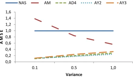
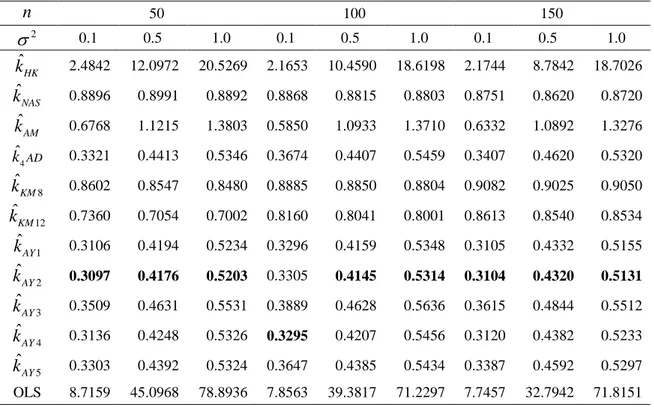
In Tables 3.1-3.6, the results of AMSE values are presented for fixed n p, , and different 2‘s. All of the proposed parameters have better performance than ˆkHK
and OLS estimator has the largest AMSE values. One can see from tables that when the error variance 2 increases, AMSE values increase for all estimators. For the casep4,0.95, kˆAY2 has the least AMSE value and other new proposed estimators except for kˆAY3 have better performance than the ones chosen from the literature.
When the degree of the correlation is increased, kˆAY5 and ˆk AD have less 4
AMSE values than other estimators for 0.99 and 0.999. One can see that all of the new proposed estimators except for kˆAY3 are quite better than the others, especially4 ˆ
AY
k is the best among them for p6 and 0.95 and 0.99. However, kˆAY5 and
4
ˆk AD perform almost equally for 0.999. Some of these results can easily be seen from Figure 3.2 and 3.3 as well. All comparison graphs have been sketched using earlier parameters kˆNAS,kˆAM,kˆ4
AD and new parameters kˆAY2,kˆAY3 selected randomly. Since the values of OLS and ˆkHK estimators are larger than the others in scale, they are not included in the graphs.It is known that multicollinearity becomes severe when the correlation increases. However, there is an interesting result that AMSE values of new proposed estimators decrease, when the correlation increases. In other words, new proposed estimators are robust to the correlation. This feature is also observed for ˆk AD and presented in the 4
Figure. 3.6.0.0 0.2 0.4 0.6 0.8 1.0 1.2 1.4 1.6 0.1 0.5 1.0 A M S E Variance
NAS AM AD4 AY2 AY3
Figure 3.2. Comparison of AMSE values for n50, 0.95, p4
Figure 3.3. Comparison of AMSE values for n150, 0.95, p4
0,0 0,2 0,4 0,6 0,8 1,0 1,2 1,4 1,6 0.1 0.5 1,0 A M S E Variance
NAS AM AD4 AY2 AY3
0.0 0.2 0.4 0.6 0.8 1.0 1.2 1.4 0.1 0.5 1.0 A M S E Variance
NAS AM AD4 AY2 AY3
Figure 3.5. Comparison of AMSE values for n150, 0.999, p6
Figure 3.6. Comparison of AMSE values for n50, 2 0.1, p4
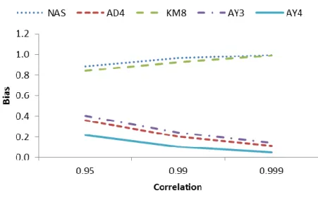
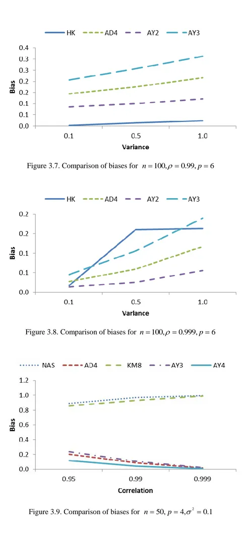
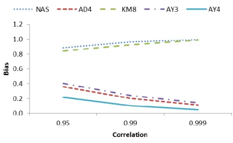
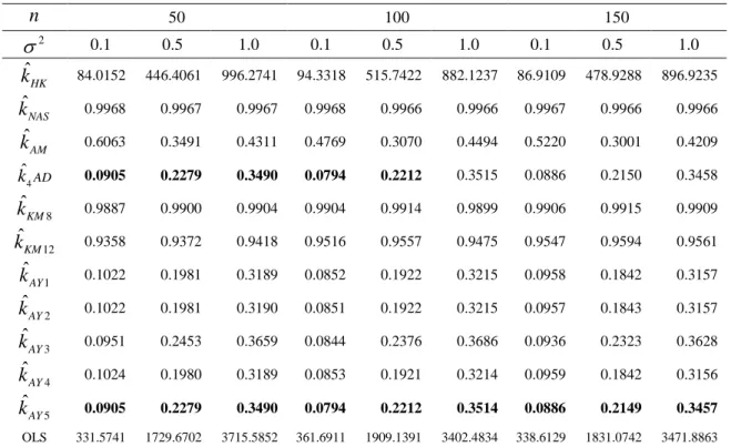
Although MSE is used as a comparison criterion, bias of an estimator is another indicator of good performance. Thus, comparisons of the estimators according to biases are summarized in Figure 3.7-3.10. In most of the cases, ˆkHK has the least bias value. If the degree of correlation is increased, estimators have more bias as it is observed from Figure. 3.7. Moreover, kˆAY2 has a less bias than ˆk AD . 4
When0.999, kˆAY2 becomes the estimator having the least bias. Also
4
ˆk AD and ˆ 4 AY
k have quite less biases for this situation. If the biases are compared to the error variance, one can see that when the error variance increases, bias values of all of the estimators except for kˆKM8 and kˆKM12 increases monotonically when 0.95
andp4. Figures 3.7-3.8, show the performances of bias values between the estimators.
Figure 3.7. Comparison of biases for n100, 0.99, p6
Figure 3.8. Comparison of biases for n100, 0.999, p6